Dynamic Mixed Modeling in Large Eddy Simulation Using the Concept of a Subgrid Activity Sensor

Abstract

Following the relative success of mixed models in the Large Eddy Simulation of complex turbulent flow configurations, an alternative formulation is suggested here which incorporates the concept of a local subgrid activity sensor. The general idea of mixed models is to combine the advantages of structural models (superior alignment properties), usually of the scale similarity type, and functional models (superior stability), usually of the eddy viscosity type, while avoiding their disadvantages. However, the key question is the mathematical realization of this combination, and the formulation in this work accounts for the local level of underresolution of the flow. The justification and evaluation of the newly proposed mixed model is based on a priori and a posteriori analysis of homogeneous isotropic turbulence and laminar–turbulent transition in the Taylor–Green vortex, respectively. The suggested model shows a robust and accurate behavior for the cases investigated. In particular, it outperforms the separate structural and functional base models as well as the simulation without an explicit subgrid-scale model.

1. Introduction

Although the scientific foundations of the Large Eddy Simulation (LES) have been explored for decades, the full potential of this flow simulation technique now unfolds in the age of high-performance computing and allows to tackle not only academic but also technical problems. Mixed models, i.e., a combination of functional and structural subgrid-scale (SGS) models, are among the most successful approaches for LES. Compared with purely structural models, mixed models are especially superior in terms of stability. In the most straight-forward formulation, the respective weights of the structural and functional parts are preset, which has obvious drawbacks. More advanced mixed models incorporate a dynamic procedure of the Germano-Lilly type [1] in order to dynamically determine the respective weights of the model contributions [2,3]. However, such approaches usually require some kind of regularization, like averaging in homogeneous directions, which limits the general applicability. A comprehensive overview of different mixed modeling strategies is provided by Sagaut [4].

Chapelier et al. [5] have recently demonstrated the potential of a subgrid activity sensor to improve the performance of functional eddy viscosity models in regions with transitional flow features. Further, it has been shown by Hasslberger et al. [6] how a subgrid activity sensor can additionally be used to rectify the incorrect near-wall scaling of eddy viscosity base models like the standard Smagorinsky model without explicit wall damping. Accordingly, the idea here is to exploit the advantages of a subgrid activity sensor in the context of mixed SGS modeling, as first attempted in [7]. The aim of the subgrid activity sensor is to determine the local level of under-resolution of the flow on the fly, i.e., during the runtime of the CFD simulation. Using this information, in a local and instantaneous sense, accurate and robust SGS modeling is facilitated.

The coherent structure function [8], as required in the following analysis, is a useful quantity to characterize the structure of turbulent flows. It is defined as $F_{CS}=Q/E$, i.e., the second invariant of the grid-scale velocity gradient tensor

$$Q=({\overline{\mathrm{\Omega }}}_{ij}{\overline{\mathrm{\Omega }}}_{ij}-{\overline{S}}_{ij}{\overline{S}}_{ij})/2$$

(1)

being normalized by its magnitude

$$E=({\overline{\mathrm{\Omega }}}_{ij}{\overline{\mathrm{\Omega }}}_{ij}+{\overline{S}}_{ij}{\overline{S}}_{ij})/2$$

(2)

where ${\overline{S}}_{ij}=(\partial {\overline{u}}_i/\partial x_j+\partial {\overline{u}}_j/\partial x_i)/2$ is the grid-scale strain tensor and ${\overline{\mathrm{\Omega }}}_{ij}=(\partial {\overline{u}}_i/\partial x_j-\partial {\overline{u}}_j/\partial x_i)/2$ is the grid-scale rotation tensor. Consequently, $F_{CS}$ exhibits a definite lower and upper limit, i.e., $-1\le F_{CS}\le +1$. The values $-1$ and $+1$ correspond to pure elongation/strain and pure rotation, respectively. It is important to note that the constituents of Q and E are related to fundamental quantities to describe turbulent flows, namely the dissipation of kinetic energy into heat per unit mass, $2\nu S_{ij}{S}_{ij}$, and enstrophy, ${\mathrm{\Omega }}_{ij}{\mathrm{\Omega }}_{ij}$.

The manuscript is organized as follows. The mathematical background and formulation of the new mixed model are presented in Section 2. This is followed by the justification of the model by means of a priori analysis in Section 3 and its evaluation by means of a posteriori analysis in Section 4. Finally, the conclusions and outlook are presented in Section 5.

2. Subgrid Scale Modeling

In the context of LES, and under the assumption of constant density and viscosity, the filtered momentum equation reads

$$\frac{\partial {\overline{u}}_i}{\partial t}+\frac{\partial {\overline{u}}_i{\overline{u}}_j}{\partial x_j}=\frac{\partial }{\partial x_j}\left(\nu \left(\frac{\partial {\overline{u}}_i}{\partial x_j}+\frac{\partial {\overline{u}}_j}{\partial x_i}\right)\right)-\frac{1}{\rho }\frac{\partial \overline{p}}{\partial x_i}-\frac{\partial {\tau }_{ij}}{\partial x_j},$$

(3)

where $\rho$, p, $\nu$ and $u_i$ denote the density, pressure, kinematic viscosity and ith component of the velocity vector, respectively. The best-known functional SGS model is the standard Smagorinsky model [9], which calculates the deviatoric part ${\tau }_{ij}^{dev}={\tau }_{ij}-\frac{1}{3}{\tau }_{kk}{\delta }_{ij}$ of the SGS stress tensor for incompressible flows, ${\tau }_{ij}=\overline{u_i{u}_j}-{\overline{u}}_i{\overline{u}}_j$, as

$${\tau }_{ij}^{EV}=-2C_{Smago}^2{\mathrm{\Delta }}^2\sqrt{2{\overline{S}}_{kl}{\overline{S}}_{kl}}{\overline{S}}_{ij}=-2{\nu }_t{\overline{S}}_{ij}$$

(4)

where $\mathrm{\Delta }$ is the grid size (i.e., the implicit filter width), ${\nu }_t$ is the eddy viscosity (EV) and $C_{Smago}=0.17$ is the theoretical value of the Smagorinsky constant.

In contrast to functional eddy viscosity models, structural models aim to reproduce the structure of the SGS stress tensor itself and, among them, the Bardina/Liu model [10,11]

$${\tau }_{ij}^{SS}=\widehat{{\overline{u}}_i{\overline{u}}_j}-\widehat{{\overline{u}}_i}{\widehat{\overline{u}}}_j$$

(5)

is based on the scale similarity (SS) principle, where $\left(\widehat{·}\right)$ represents a suitably defined explicit test filter. In this work, the explicit test filter for any field quantity ${\varphi }_{i,j,k}$ at the discrete location given by the index triple ($i,j,k$) is implemented according to Anderson and Domaradzki [12]:

$${\widehat{\varphi }}_{i,j,k}=\sum _{l=-1}^{+1}\sum _{m=-1}^{+1}\sum _{n=-1}^{+1}{b}_l·b_m·b_n·{\varphi }_{i+l,j+m,k+n}$$

(6)

This three-dimensional filter is the product of the convolution of three one-dimensional filters with coefficients $(b_{-1},b_0,b_{+1})=(c^{fil},1-2c^{fil},c^{fil})$. Hence, only the considered cell itself and direct neighbor cells $(l,m,n\in \{-1,0,+1\left\}\right)$ are taken into account by different weights, which makes the test filtering procedure computationally inexpensive. A filter coefficient of $c^{fil}=1/12$ is chosen here in agreement with the recommendation by Anderson and Domaradzki [12]. In principle, the results of the Bardina model depend on the definition of the test filter, but the sensitivity is not large and the main advantages of this structural model are present also for other values of $c^{fil}$. This choice can be seen as a compromise between the extremes, i.e., the largest reasonable value ($c^{fil}=1/3$), which corresponds to an explicit-to-implicit filter width ratio of $\sqrt{8}$, and the smallest reasonable value ($c^{fil}=1/24$), which corresponds to an explicit-to-implicit filter width ratio of unity; see also Equation (10).

A viable alternative for the structural model is the gradient model by Clark et al. [13],

$${\tau }_{ij}^{SS}=\frac{{\mathrm{\Delta }}^2}{12}\frac{\partial {\overline{u}}_i}{\partial x_k}\frac{\partial {\overline{u}}_j}{\partial x_k},$$

(7)

which is based on a truncated Taylor-series expansion of the scale similarity model.

The following blending scheme is based on the below observation that structural models of the scale similarity (SS) type perform the best for moderate under-resolution of the flow, whereas the concept of eddy viscosity (EV) becomes increasingly valid the lower the relative resolution is. Hence, the idea is to retain the superior alignment properties of SS models in the regions where an extrapolation based on the smallest resolved scales (which are also strongly affected by numerical errors) is still properly working and to blend in a more robust EV model where physically plausible. Using a local subgrid activity sensor $\mathrm{\Theta }$, the blending scheme reads

$${\tau }_{ij}^{mixed,sensor}={\tau }_{ij}^{EV}\mathrm{\Theta }+{\tau }_{ij}^{SS}(1-\mathrm{\Theta })$$

(8)

where ${\tau }_{ij}^{EV}$ and ${\tau }_{ij}^{SS}$ represent any kind of eddy viscosity and scale similarity type model, respectively. The lower the relative resolution, the higher the subgrid activity $\mathrm{\Theta }$ and the higher (lower) the EV (SS) contribution. This is also consistent from a physical point of view, because “randomly” fluctuating incoherent turbulence acts like diffusive motion in a statistical sense [14,15,16]—agreeing with the way eddy viscosity is reflected in the diffusive term of the filtered Navier–Stokes equations.

The bounded sensor function $\mathrm{\Theta }$ is constructed as

$$\begin{array}{cc}\hfill \mathrm{\Theta }& =\left\{\begin{array}{cc}\begin{array}{cc}\hfill & 1\hfill \\ \hfill & \frac{1}{2}\left(1+sin\left(\pi \frac{{\sigma }_{eq}-2\sigma +1}{2(1-{\sigma }_{eq})}\right)\right)\hfill \\ \hfill & 0\hfill \end{array}\hfill & \mathrm{if}\begin{array}{cc}\hfill & \sigma <{\sigma }_{eq}\hfill \\ \hfill & \sigma \in [{\sigma }_{eq},1]\hfill \\ \hfill & \sigma >1\hfill \end{array}\hfill \end{array}\right.\hfill \end{array}$$

(9)

such that a smooth transition between well-resolved ($\sigma >1$) and insufficiently resolved ($\sigma <{\sigma }_{eq}$) regions is obtained. Although Equation (9) is the same as in [5], $\sigma$ is calculated in a different manner. Rather than using enstrophy only, $\sigma =\widehat{E}/E$ accounts for both dissipation and enstrophy. Comparison of the implicitly grid-filtered value E and the explicitly test-filtered value $\widehat{E}$ allows to estimate the local subgrid activity. At the same time, the intensity-preserving ($E\approx$ const.; $\widehat{E}\approx$ const.) natural exchange between dissipation and enstrophy in turbulent flows remains undetected by the sensor. According to the definition of E, Equation (2), fluctuations in strain- and rotation-dominated flow regions can be equally well reflected by the sensor. This is demonstrated in Figure 1, which depicts conditionally averaged values of the subgrid activity $\mathrm{\Theta }$ in homogeneous isotropic turbulence (details on this a priori analysis are provided subsequently). The original sensor formulation based on enstrophy only (left panel of Figure 1) is apparently unable to detect subgrid activity in strain-dominated flow regions. Strain-dominated flow regions are even more probable than rotation-dominated flow regions in turbulent flows, as demonstrated by the skewed probability density function (PDF) of the coherent structure function $F_{CS}$ in Figure 2, which shows a universal shape independent of the implicit filter width in LES. Agreeing with expectations, Figure 1 demonstrates increasing levels of subgrid activity $\mathrm{\Theta }$ for increasing under-resolution of the flow, as specified by $\mathrm{\Delta }/{\mathrm{\Delta }}_{DNS}$.

The calculation of the equilibrium value ${\sigma }_{eq}$ is identical to Chapelier et al. [5], since dissipation and enstrophy are obeying the same spectral scaling. Both spectra are proportional to ${\kappa }^{2}e\left(\kappa \right)$, with wavenumber $\kappa$ and energy spectrum $e\left(\kappa \right)$. Their peak is located at high wavenumbers (small scales), hence allow to determine the subgrid activity. On average, $\widehat{E}<E$ in the inertial subrange. The equilibrium value is given by

$${\sigma }_{eq}={\left(\frac{\widehat{\mathrm{\Delta }}}{\mathrm{\Delta }}\right)}^{-4/3}={\left(\sqrt{24c^{fil}}\right)}^{-4/3}$$

(10)

where the ratio of explicit-to-implicit filter width $\widehat{\mathrm{\Delta }}/\mathrm{\Delta }$ was further reduced to the filter coefficients, following Lund [17]. For the explicit test filter applied here, $c^{fil}=1/12$ yields ${\sigma }_{eq}=2^{-2/3}\approx 0.63$.

3. A Priori Analysis

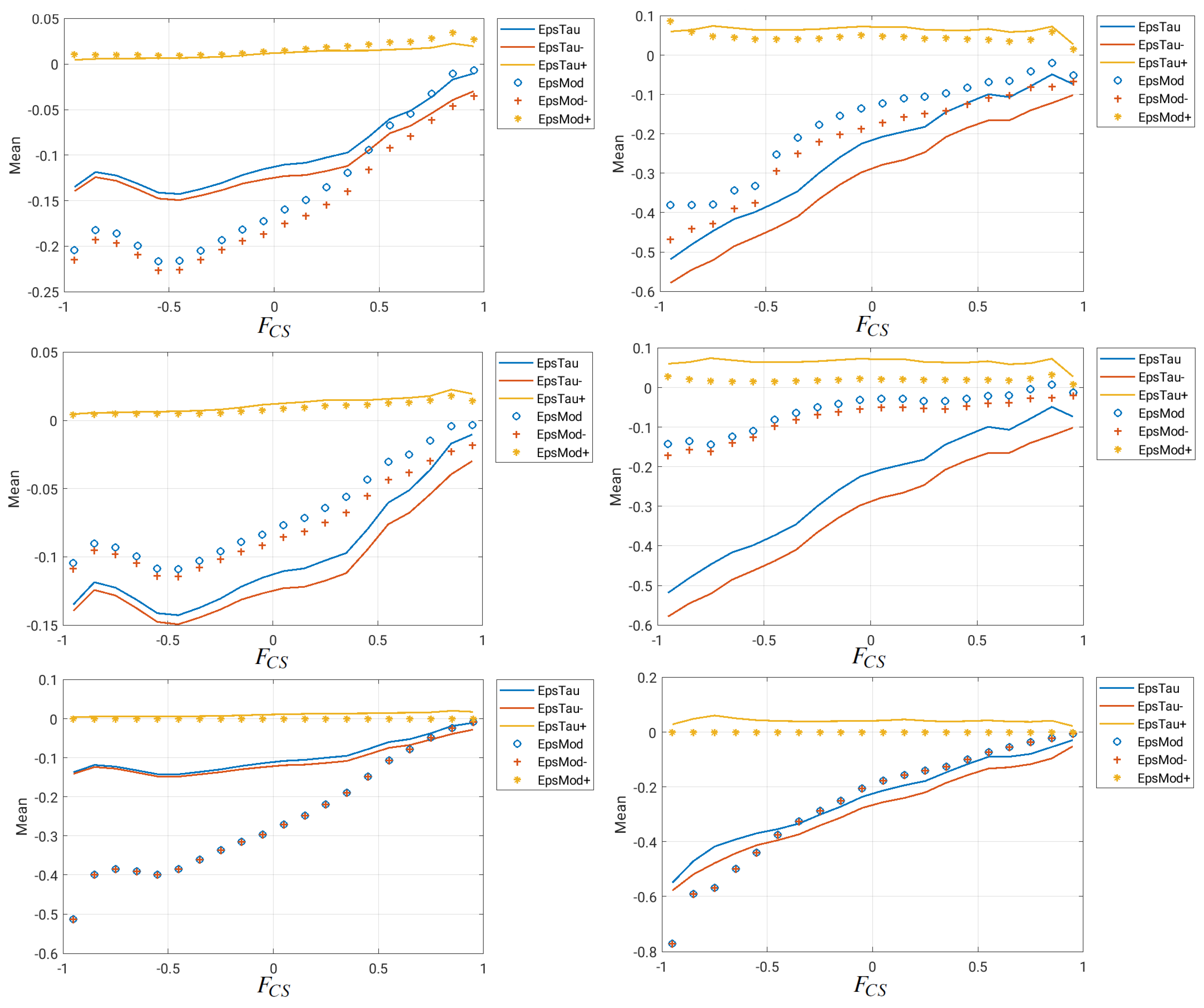
To justify the above mixed modeling idea, the SGS energy transfer behavior of the separate functional and structural base models is analyzed by means of an a priori analysis. The comparably well-defined state of homogeneous isotropic turbulence (closely resembled by the final stage of the Taylor–Green vortex, cf. $t=25$ in Figure 5) is chosen for this purpose. The Direct Numerical Simulation (DNS) database, uniformly discretized by ${512}^3$ grid points, was explicitly filtered using a Gaussian filter kernel for varying normalized filter width $\mathrm{\Delta }/{\mathrm{\Delta }}_{DNS}$. It is particularly instructive to analyze the performance conditional on the coherent structure function $F_{CS}$ due to the intricate dissipation–enstrophy interplay in turbulent flows. Also, the SGS energy transfer $ϵ={\tau }_{ij}{\overline{S}}_{ij}$ can be decomposed into forward scatter ${ϵ}^{-}=0.5(ϵ-|ϵ\left|\right)$ and backward scatter ${ϵ}^{+}=0.5(ϵ+|ϵ\left|\right)$. For consistency, only the deviatoric part of the SGS stress is considered for the EV model, although the discrepancy between ${\tau }_{ij}^{dev}={\tau }_{ij}-\frac{1}{3}{\tau }_{kk}{\delta }_{ij}$ and ${\tau }_{ij}$ is small here.

Figure 3 shows that for moderate filter width ($\mathrm{\Delta }/{\mathrm{\Delta }}_{DNS}=9$), the Bardina/Liu model and the Clark model clearly outperform the Smagorinsky model, because the latter is overly dissipative. For large filter width ($\mathrm{\Delta }/{\mathrm{\Delta }}_{DNS}=33$), only the Smagorinsky model is in good agreement with the reference data, whereas the structural models exhibit insufficient SGS energy transfer—especially the model by Clark et al. Under these conditions, the SGS energy transfer, on average, is almost linearly increasing from rotation- to strain-dominated regions, and this can be well represented by the Smagorinsky model. Although not explicitly shown here, tendencies with respect to Reynolds number variation are expected to be similar to filter width variation. It cannot be seen from this a priori analysis, but it is known that structural models tend to become unstable under high filter width/Reynolds number conditions, which motivates the mixed model. It is worth noting that the SS models are able to represent backward scatter in contrast to the EV model. Backward scatter is not unphysical, as shown in this a priori analysis, but it is discussed as a potential source of instability for structural models in the literature [18,19]. However, it is only a hypothesis, without clear proof, that the structural model instability comes (solely) from backscatter. As an alternative view, the instability may come from the massively under-resolved regions (which are also strongly affected by numerical errors in LES), and a robust eddy viscosity model is used in such regions with the proposed mixed model according to Equation (8). Based on the subsequent a posteriori results in Section 4, it seems unnecessary with the proposed mixed model, but one could easily remove the backscatter by setting the model contribution to zero locally if the SGS energy transfer ${\tau }_{ij}^{model}{\overline{S}}_{ij}>0$.

The superior alignment properties of structural models compared with functional models, as mentioned before, are evident from Figure 4. For this purpose, the Pearson correlation coefficients between the “true” SGS stress tensor ${\tau }_{ij}^{DNS}$ and the model tensor ${\tau }_{ij}^{model}$ before (independent components xx, yy, zz, xy, xz and yz) and after taking the divergence (independent components DivX, DivY and DivZ) are evaluated conditional on the coherent structure function $F_{CS}$. According to the Cauchy–Schwarz inequality, this correlation coefficient assumes values between $-1$ and $+1$, where $+1$ is a total positive linear correlation, 0 is no linear correlation and $-1$ is a total negative linear correlation. Also, note that the closure term in the filtered Navier–Stokes equations involves the divergence operator, i.e., $\partial {\tau }_{ij}/\partial x_j$, and the centered derivatives in this a priori analysis are based on the corresponding LES grid. It can be hypothesized that the correlation decrease for structural models and after taking the divergence towards the rotation-dominated side ($F_{CS}>0$) is due to the fact that the high-vorticity structures are spatially concentrated, which leads to increasing differentiation errors. Such structures are often referred to as vortex tubes and are a key characteristic of turbulent flows. Generally, the correlation coefficients are higher for the structural models, which is a manifestation of their superior alignment properties. This advantage over functional models is very clear for moderate filter width ($\mathrm{\Delta }/{\mathrm{\Delta }}_{DNS}=9$) but almost disappears for large filter width ($\mathrm{\Delta }/{\mathrm{\Delta }}_{DNS}=33$), i.e., strong under-resolution of the flow. In contrast, the correlation coefficients for the functional model are rather independent of the filter width. Due to the eddy viscosity model base formulation, ${\tau }_{ij}=-2{\nu }_t{\overline{S}}_{ij}$, the correlation coefficients are somewhat higher in strain-dominated flow regions ($F_{CS}<0$). Consistent with these observations, the eddy viscosity concept is increasingly valid for increasing filter width, hence in a statistical sense, whereas it is inappropriate in a local and instantaneous sense.

4. A Posteriori Analysis

The open-source code PARIS [20] was employed to solve the unsteady incompressible Navier–Stokes equations. It uses a second-order Runge–Kutta technique for time integration, and spatial discretization is realized by the finite-volume approach on a uniform, cubic staggered grid with second-order centered difference schemes for both convective and diffusive fluxes. In the framework of the projection method, the pressure field is calculated by a multigrid Poisson solver provided by the HYPRE library.

The Taylor–Green vortex [21] is a challenging test case for laminar–turbulent transition, and this configuration consists of a cube with side length of $2\pi$ and periodic boundaries in all directions. The velocity field is initialized as

$$\begin{array}{ccc}\hfill u(x,y,z)& =cos\left(x\right)sin\left(y\right)sin\left(z\right)\hfill & \hfill \end{array}$$

(11)

$$\begin{array}{cc}\hfill v(x,y,z)& =-sin\left(x\right)cos\left(y\right)sin\left(z\right)\hfill \end{array}$$

(12)

$$\begin{array}{ccc}w(x,y,z)\hfill & =0\hfill & \hfill \hspace{1em}\hspace{1em}\hspace{1em}\hspace{1em}\hspace{1em}\hspace{1em}\hspace{1em}\hspace{1em}\end{array}$$

(13)

Referring to the initial state, the Reynolds number is 1600, and the density is assumed to be constant. Two different resolutions were investigated, i.e., the benchmark DNS and a much coarser uniform ${32}^3$ grid for all a posteriori LES runs. A constant nondimensional time step size of $0.003$ was chosen such that the Courant number is at least one order of magnitude below unity during the entire simulation period. In this way, the numerical dissipation due to the time integration scheme is negligible and therefore not masking the effect of the explicit turbulence model. A maximum of only two pressure iterations is required within the framework of the multigrid Poisson solver. For each individual LES run, the computational cost is approximately 0.8 CPU-hours, which were executed on a single Intel Xeon CPU core (E5-2640 at 2 GHz). Hence, the LES setup can be considered computationally very efficient. There is a possibility of speeding up the simulations with adaptive time stepping, but this is largely independent from subgrid-scale modeling, which is the main topic of this paper. The nondimensional simulation time ranges from $t=0$ to $t=25$, and the corresponding development of the flow in the DNS is shown in Figure 5. Through vortex stretching and breakdown, the flow evolves from a quasi-laminar initial condition to fairly homogeneous fully developed turbulence at the final stage considered.

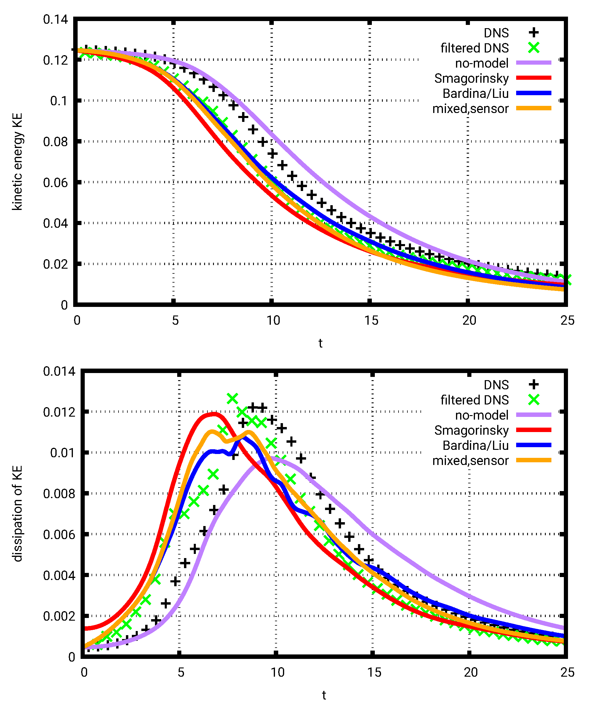
Figure 6 shows the temporal evolution of the mean kinetic energy and its dissipation rate for the no-model LES, the Smagorinsky model, the Bardina/Liu model and the sensor-based mixed model. Both the filtered and unfiltered DNS results are included as references. As expected, the EV model itself is overly dissipative during the quasi-laminar initial stage. The SS model itself underpredicts the peak dissipation and shows first signs of instability, i.e., unnatural oscillations of the dissipation curve, during the high-dissipation phase around $5<t<15$. In contrast, the sensor-based mixed model correctly reduces to the filtered DNS in the initial stage, improves the peak dissipation and also appears to be more robust during the high-dissipation phase. In a situation where $\sigma \ge 1$ and consequently $\mathrm{\Theta }=0$, only the structural part of the mixed model is active according to Equation (8). It is a great advantage of the scale similarity type models that they reduce correctly to the no-model LES (i.e., their contribution vanishes) for fully resolved flow conditions. This situation can indeed be seen here for the quasi-laminar initial condition, where the overall mixed model vanishes, because the structural model contribution also vanishes. Exploitation of such natural asymptotic behavior of the SS base model is different from the original approach of Chapelier et al. [5], where only a functional model contribution was considered. A clear improvement compared with the no-model LES can be observed as well. Note that relatively increased dissipation in early stages can lead to relatively decreased dissipation in late stages of the TGV—and vice versa. The timing matters in this transient, which makes it a challenging test case for SGS modeling.

The difference between the original sensor by Chapelier et al. [5] based on grid-scale enstrophy (${\overline{\mathrm{\Omega }}}_{ij}{\overline{\mathrm{\Omega }}}_{ij}$) and the present modified sensor based on the sum of grid-scale enstrophy and dissipation ($E=({\overline{\mathrm{\Omega }}}_{ij}{\overline{\mathrm{\Omega }}}_{ij}+{\overline{S}}_{ij}{\overline{S}}_{ij})/2$) can be discerned from Figure 7. Although the overall results are quite similar, the mixed model using the newly proposed sensor is somewhat less oscillatory, which can be seen especially during the high-dissipation phase around $5<t<15$. The modified sensor variant based on E is thus recommended and used as a default in the following.

Figure 8 depicts the temporal evolution of the maximum and volume average of the subgrid activity $\mathrm{\Theta }$ for the mixed model using the original sensor based on enstrophy only and the mixed model using the newly proposed sensor based on the sum of enstrophy and dissipation. As expected, the subgrid activity, equivalent to the level of under-resolution of the flow, is zero at the beginning of the simulation, because the initial condition of the Taylor–Green vortex consists of a long-wavelength perturbation only, which can be fully resolved even on the coarse LES grid. During the process of laminar–turbulent transition, both the maximum and volume average of $\mathrm{\Theta }$ increase considerably before remaining at a saturated level for the rest of the simulation. This is consistent with the fact that the smallest turbulent structures at the Kolmogorov scale can obviously not be resolved by the coarse LES grid, hence necessitating SGS energy drain. Despite the comparably low mean value of $\mathrm{\Theta }$ in the saturated phase, between $7\%$ and $15\%$ depending on the sensor formulation, it appears that the EV part of the mixed model is introduced just at the right locations to stabilize the simulation. The maximum value of $\mathrm{\Theta }$ in the saturated phase, between $90\%$ and $100\%$, reveals that in the critical regions, the structural model is (almost) entirely replaced by the functional model according to Equation (8). Furthermore, it is interesting to note that the present sensor formulation shows improved robustness compared with the original sensor formulation (Figure 7), although the mean value of $\mathrm{\Theta }$, and therefore the percentage of the EV part, is larger in the latter case. The reason for this observation is the different spatial distribution of the stabilizing eddy viscosity contribution, which is potentially more reasonable with the present sensor formulation. As an example, the original sensor does not allow for eddy viscosity addition in strongly strain-dominated flow regions due to its enstrophy-based construction. However, the a priori analysis in this paper shows clearly, especially for large filter widths, that most of the SGS energy transfer is needed in strain-dominated flow regions, as characterized by $F_{CS}<0$ in Figure 3, and this is facilitated with the present sensor formulation based on enstrophy and dissipation.

Replacing the Bardina/Liu model with the gradient model by Clark et al., the sensor-based mixed model again leads to a clear improvement over the separate structural model, as can be seen in Figure 9. As expected, the curves start to diverge considerably when the level of under-resolution becomes significant at $t\approx 4$. In this case, the improvement through the sensor-based regularization is even more obvious than with the Bardina/Liu model combination (Figure 6).

5. Conclusions and Outlook

A strategy for mixed modeling in LES is proposed by means of a subgrid activity sensor-based blending between the functional and structural base models. This mixed model outperforms the separate base models (here: Bardina/Liu or Clark and Smagorinsky) for the Taylor–Green vortex test case, and it is oscillation-free without additional regularization like averaging (in homogeneous direction), relaxation in time or clipping (of backscatter). It is worth noting that the overall model is also parameter-free, apart from the choice of the test filter.

Since it is not discussed here, future work will focus on the wall treatment for the proposed mixed model. This can be achieved either by replacing the current base models with models that already incorporate the correct wall scaling, e.g., [22,23], or by using a wall-scaling sensor, e.g., [6], in addition to the non-wall-scaling sensor $\mathrm{\Theta }$ for blending. Note that the structural models by Bardina/Liu et al. and Clark et al. also suffer from incorrect near-wall scaling [24].

References

- Lilly, D.K. A proposed modification of the Germano subgrid-scale closure method. Phys. Fluids A Fluid Dyn. 1992, 4, 633–635. [Google Scholar] [CrossRef]
- Zang, Y.; Street, R.L.; Koseff, J.R. A dynamic mixed subgrid-scale model and its application to turbulent recirculating flows. Phys. Fluids A Fluid Dyn. 1993, 5, 3186–3196. [Google Scholar] [CrossRef]
- Sagaut, P.; Garnier, E.; Terracol, M. A general algebraic formulation for multi-parameter dynamic subgrid-scale modeling. Int. J. Comput. Fluid Dyn. 2000, 13, 251–257. [Google Scholar] [CrossRef]
- Sagaut, P. Large Eddy Simulation for Incompressible Flows: An Introduction; Springer Science & Business Media: Berlin/Heidelberg, Germany, 2005. [Google Scholar]
- Chapelier, J.B.; Wasistho, B.; Scalo, C. A Coherent vorticity preserving eddy-viscosity correction for Large-Eddy Simulation. J. Comput. Phys. 2018, 359, 164–182. [Google Scholar] [CrossRef] [Green Version]
- Hasslberger, J.; Engelmann, L.; Kempf, A.; Klein, M. Robust dynamic adaptation of the Smagorinsky model based on a sub-grid activity sensor. Phys. Fluids 2021, 33, 015117. [Google Scholar] [CrossRef]
- Hasslberger, J. A sub-grid activity sensor applied to mixed modeling in large eddy simulation. In Proceedings of the 12th International Symposium on Turbulence and Shear Flow Phenomena, Osaka, Japan, 19–22 July 2022. [Google Scholar]
- Kobayashi, H. The subgrid-scale models based on coherent structures for rotating homogeneous turbulence and turbulent channel flow. Phys. Fluids 2005, 17, 045104. [Google Scholar] [CrossRef]
- Smagorinsky, J. General circulation experiments with the primitive equations: I. The basic experiment. Mon. Weather. Rev. 1963, 91, 99–164. [Google Scholar] [CrossRef]
- Bardina, J. Improved Turbulence Models Based on Large Eddy Simulation of Homogeneous, Incompressible, Turbulent Flows. Ph.D. Thesis, Stanford University, Stanford, CA, USA, 1983. [Google Scholar]
- Liu, S.; Meneveau, C.; Katz, J. On the properties of similarity subgrid-scale models as deduced from measurements in a turbulent jet. J. Fluid Mech. 1994, 275, 83–119. [Google Scholar] [CrossRef]
- Anderson, B.; Domaradzki, J. A subgrid-scale model for large-eddy simulation based on the physics of interscale energy transfer in turbulence. Phys. Fluids 2012, 24, 065104. [Google Scholar] [CrossRef]
- Clark, R.; Ferziger, J.; Reynolds, W. Evaluation of subgrid-scale models using an accurately simulated turbulent flow. J. Fluid Mech. 1979, 91, 1–16. [Google Scholar] [CrossRef]
- Farge, M. Wavelet transforms and their applications to turbulence. Annu. Rev. Fluid Mech. 1992, 24, 395–458. [Google Scholar] [CrossRef]
- Farge, M.; Pellegrino, G.; Schneider, K. Coherent vortex extraction in 3D turbulent flows using orthogonal wavelets. Phys. Rev. Lett. 2001, 87, 054501. [Google Scholar] [CrossRef] [PubMed] [Green Version]
- Bockhorn, H.; Denev, J.A.; Domingues, M.; Falconi, C.; Farge, M.; Fröhlich, J.; Gomes, S.; Kadoch, B.; Molina, I.; Roussel, O.; et al. Numerical simulation of turbulent flows in complex geometries using the coherent vortex simulation approach based on orthonormal wavelet decomposition. In Numerical Simulation of Turbulent Flows and Noise Generation: Results of the DFG/CNRS Research Groups FOR 507 and FOR 508; Springer: Berlin/Heidelberg, Germany, 2009; pp. 175–200. [Google Scholar]
- Lund, T. On the use of discrete filters for large eddy simulation. Annu. Res. Briefs 1997, 83–95. [Google Scholar]
- Kobayashi, H. Improvement of the SGS model by using a scale-similarity model based on the analysis of SGS force and SGS energy transfer. Int. J. Heat Fluid Flow 2018, 72, 329–336. [Google Scholar] [CrossRef]
- Klein, M.; Ketterl, S.; Engelmann, L.; Kempf, A.; Kobayashi, H. Regularized, parameter free scale similarity type models for Large Eddy Simulation. Int. J. Heat Fluid Flow 2020, 81, 108496. [Google Scholar] [CrossRef]
- Aniszewski, W.; Arrufat, T.; Crialesi-Esposito, M.; Dabiri, S.; Fuster, D.; Ling, Y.; Lu, J.; Malan, L.; Pal, S.; Scardovelli, R.; et al. Parallel, robust, interface simulator (PARIS). Comput. Phys. Commun. 2021, 263, 107849. [Google Scholar] [CrossRef]
- Brachet, M.; Meiron, D.; Orszag, S.; Nickel, B.; Morf, R.; Frisch, U. Small-scale structure of the Taylor–Green vortex. J. Fluid Mech. 1983, 130, 411–452. [Google Scholar] [CrossRef] [Green Version]
- Nicoud, F.; Toda, H.; Cabrit, O.; Bose, S.; Lee, J. Using singular values to build a subgrid-scale model for large eddy simulations. Phys. Fluids 2011, 23, 085106. [Google Scholar] [CrossRef] [Green Version]
- Trias, F.; Folch, D.; Gorobets, A.; Oliva, A. Building proper invariants for eddy-viscosity subgrid-scale models. Phys. Fluids 2015, 27, 065103. [Google Scholar] [CrossRef] [Green Version]
- Silvis, M.; Remmerswaal, R.; Verstappen, R. Physical consistency of subgrid-scale models for large-eddy simulation of incompressible turbulent flows. Phys. Fluids 2017, 29, 015105. [Google Scholar] [CrossRef] [Green Version]
Figure 1.
Homogeneous isotropic turbulence: Means of the subgrid activity sensor conditional on the coherent structure function , where and correspond to pure strain and pure rotation, respectively. Results are shown for filter width 3 (blue), 5 (red), 9 (yellow), 13 (purple) and 17 (green). Original formulation based on enstrophy on the left, present formulation based on enstrophy and dissipation on the right.
Figure 2.
Homogeneous isotropic turbulence: Probability density function (PDF) of the coherent structure function , where and correspond to pure strain and pure rotation, respectively. Results are shown for filter width 3 (blue), 5 (red), 9 (yellow), 13 (purple) and 17 (green).
Figure 3.
Homogeneous isotropic turbulence: Means of the “true” SGS energy transfer (EpsTau, continuous lines) and model energy transfer (EpsMod, marker symbols) conditional on the coherent structure function . Eps- and Eps+ indicate forward scatter and backward scatter . Results are shown for the Bardina/Liu model (first row), Clark model (second row) and Smagorinsky model (third row) for moderate, i.e., (left), and large filter widths, i.e., (right), respectively. Note the different scales of the ordinate axes.
Figure 4.
Homogeneous isotropic turbulence: Pearson correlation coefficient between the “true” SGS stress tensor and the model tensor before (xx, yy, zz, xy, xz and yz) and after taking the divergence (DivX, DivY and DivZ), conditional on the coherent structure function . Results are shown for the Bardina/Liu model (first row), Clark model (second row) and Smagorinsky model (third row) for moderate, i.e., (left), and large filter widths, i.e., (right), respectively.
Figure 5.
Stages of the Taylor–Green vortex as seen in the reference DNS: Instantaneous views of iso-contours colored by the velocity magnitude at nondimensional simulation times t = 2.5, 5, 7.5, 10, 15 and 25.
Figure 6.
Taylor–Green vortex: Volume-averaged kinetic energy (top) and its dissipation rate (bottom) versus nondimensional time for the reference DNS, the no-model LES, the Smagorinsky model, the Bardina/Liu model and the sensor-based mixed model.
Figure 7.
Taylor–Green vortex: Volume-averaged kinetic energy (top) and its dissipation rate (bottom) versus nondimensional time for the reference DNS, the no-model LES, the mixed model using the original sensor based on enstrophy only and the mixed model using the newly proposed sensor based on the sum of enstrophy and dissipation.
Figure 8.
Taylor–Green vortex: Maximum and volume average of the subgrid activity sensor versus nondimensional time for the mixed model using the original sensor based on enstrophy only and the mixed model using the newly proposed sensor based on the sum of enstrophy and dissipation.
Figure 9.
Taylor–Green vortex: Volume-averaged kinetic energy (top) and its dissipation rate (bottom) versus nondimensional time for the reference DNS, the no-model LES, the separate model by Clark et al. and the sensor-based mixed model using the structural model by Clark et al. instead of Bardina/Liu et al.
Disclaimer/Publisher’s Note: The statements, opinions and data contained in all publications are solely those of the individual author(s) and contributor(s) and not of MDPI and/or the editor(s). MDPI and/or the editor(s) disclaim responsibility for any injury to people or property resulting from any ideas, methods, instructions or products referred to in the content. |
© 2023 by the author. Licensee MDPI, Basel, Switzerland. This article is an open access article distributed under the terms and conditions of the Creative Commons Attribution (CC BY) license (https://creativecommons.org/licenses/by/4.0/).
Share and Cite
MDPI and ACS Style
Hasslberger, J. Dynamic Mixed Modeling in Large Eddy Simulation Using the Concept of a Subgrid Activity Sensor. Fluids 2023, 8, 219. https://doi.org/10.3390/fluids8080219
AMA Style
Hasslberger J. Dynamic Mixed Modeling in Large Eddy Simulation Using the Concept of a Subgrid Activity Sensor. Fluids. 2023; 8(8):219. https://doi.org/10.3390/fluids8080219
Chicago/Turabian StyleHasslberger, Josef. 2023. "Dynamic Mixed Modeling in Large Eddy Simulation Using the Concept of a Subgrid Activity Sensor" Fluids 8, no. 8: 219. https://doi.org/10.3390/fluids8080219