

Transition to Equilibrium and Coherent Structure in Ideal MHD Turbulence, Part 2


Department of Physics and Astronomy, George Mason University, Fairfax, VA 22030, USA
Fluids 2023, 8(6), 181; https://doi.org/10.3390/fluids8060181
Submission received: 10 May 2023
/
Revised: 7 June 2023
/
Accepted: 12 June 2023
/
Published: 14 June 2023
(This article belongs to the Special Issue Fluids in Magnetic/Electric Fields, 2nd Edition)
Abstract
:We continue our study of the transition of ideal, homogeneous, incompressible, magnetohydrodynamic (MHD) turbulence from non-equilibrium initial conditions to equilibrium using long-time numerical simulations on a periodic grid. A Fourier spectral transform method is used to numerically integrate the dynamical equations forward in time. The six runs that previously went to near equilibrium are here extended into equilibrium. As before, we neglect dissipation as we are primarily concerned with behavior at the largest scale where this behavior has been shown to be essentially the same for ideal and real (forced and dissipative) MHD turbulence. These six runs have various combinations of imposed rotation and mean magnetic field and represent the five cases of ideal, homogeneous, incompressible, and MHD turbulence: Case I (Run 1), with no rotation or mean field; Case II (Runs 2a and 2b), where only rotation is imposed; Case III (Run 3), which has only a mean magnetic field; Case IV (Run 4), where rotation vector and mean magnetic field direction are aligned; and Case V (Run 5), which has non-aligned rotation vector and mean field directions. Statistical mechanics predicts that dynamic Fourier coefficients are zero-mean random variables, but largest-scale coherent magnetic structures emerge and manifest themselves as Fourier coefficients with very large, quasi-steady, mean values compared to their standard deviations, i.e., there is ‘broken ergodicity.’ These magnetic coherent structures appeared in all cases during transition to near equilibrium. Here, we report that, as the runs were continued, these coherent structures remained quasi-steady and energetic only in Cases I and II, while Case IV maintained its coherent structure but at comparatively low energy. The coherent structures that appeared in transition in Cases III and V were seen to collapse as their associated runs extended into equilibrium. The creation of largest-scale, coherent magnetic structure appears to be a dynamo process inherent in ideal MHD turbulence, particularly in Cases I and II, i.e., those cases most pertinent to planets and stars. Furthermore, the statistical theory of ideal MHD turbulence has proven to apply at the largest scale, even when dissipation and forcing are included. This, along with the discovery and explanation of dynamically broken ergodicity, is essentially a solution to the ‘dynamo problem’.
1. Introduction
The ‘dynamo problem’ is the problem of understanding how magnetofluids within planets and stars produce a quasi-stationary, energetic dipole magnetic field. Over a century ago, Larmor [1] hypothesized that the solution lay in a ‘self-excited dynamo’ within the Earth or the Sun. The conjectured dynamo was not mechanical, like Faraday’s dynamo, but was thought to arise from ‘convective circulation’ and ‘electric currents.’ Four decades later, Elsässer [2] saw that for ‘the dynamo problem, that is … the problem of generating and maintaining magnetic fields which draw their energy from the mechanical energy of the fluid, the nonlinear character of the equations is altogether essential’, as it produces ‘turbulence, the most conspicuous of the nonlinear phenomena of fluid dynamics.’ Thus, he realized that statistically stationary hydromagnetic turbulence was fundamental to the solution of the dynamo problem, rather than ‘rigorously stationary flow’ (i.e., a kinematic dynamo). He added that there were ‘qualitative conditions, three in number, requisite for the operation of … dynamo models’; these conditions were (1) large linear dimensions; (2) rotation; and (3) convection. The first condition implies that Reynolds numbers are sufficiently large; the second that rotation axis and magnetic dipole vector appear on average to be aligned in planets and stars; and the third, that convection is the dynamo’s source of energy. MHD turbulence, due to conditions (1) and (3), is expected to occur in planetary liquid cores and stellar interiors when global magnetism is observed, and must be an integral part of any dynamo model. Condition (2), rotation, appears to cause a close alignment between the dipole moment vector and the rotation axis; however, despite being prevalent in planets and stars, is not essential for dynamo action, whereas MHD turbulence is. Our conclusion, as discussed herein, is that MHD turbulence is the dynamo.
Earth is the primary example we have of a planet with a quasi-steady, mostly dipole magnetic field; current knowledge about the external geomagnetic field is contained in the International Geomagnetic Reference Field [3]. Reynolds numbers are predicted to be very large within the Earth’s outer core, so that convective forcing is able to produce MHD turbulence, which must be involved in creating and maintaining the geodynamo [4]. The realistic numerical simulations of the geodynamo [5,6,7], by including dissipation and forcing, have established that MHD processes within the Earth are capable of creating a magnetic field similar to the actual geomagnetic field, including the reversals of the dominant dipole component. There have also been laboratory experiments involving magnetofluids [8], some of which have shown the growth of a self-generated magnetic field, i.e., a dynamo effect [9,10,11]. Thus, the ‘dynamo problem’ falls within the purview of MHD theory, experiment and computation. However, in spite of successful numerical simulations and laboratory experiments, the fundamental origin of the geomagnetic dipole field still appeared to be a theoretical mystery [12]. Here, we present results aimed at resolving this mystery. Our focus will be on ideal MHD theory and computation as this allows us to examine large-scale dynamics without the complications of dissipation and forcing, or the associated artefacts that arise in sub-grid scale modeling.
In that regard, our new results come from extending into equilibrium the numerical simulations reported in [13], where relevant background and references are given. In brief, we use a Fourier spectral transform method as a surrogate for a planetary interior that contains a turbulent magnetofluid, such as the Earth’s outer core. The connection between the periodic box of a Fourier model and the spherical shell of an Earth-like model is that they have essentially the same ideal MHD statistical mechanics [14]. However, no spectral transform methods for studying MHD turbulence in a spherical shell exist yet, and although non-transform methods [15,16,17] have been used, they will always have insufficient resolution. Thus, we use Fourier spectral transform methods in a periodic box because they are efficient and, again, serve as a surrogate for transform methods more explicitly designed for spherical shells, until such methods are available.
In our previous computer runs [13], the transition of ideal MHD turbulence from non-equilibrium initial conditions to near equilibrium was studied and the results showed that a quasi-steady, energetic, coherent structure (equivalent to a dipole magnetic field) arose in all the cases defined in Table 1. The appearance of coherent structure is an example of ‘broken ergodicity’ [18]. As explained in the Appendix to [13], ergodicity is dynamically broken when some of the largest-scale magnetic Fourier coefficients become very large, as statistically predicted, and then become essentially constant as they are slightly affected by the myriad of very small random perturbations due to all the other Fourier modes.
However, these coherent structures were not statistically expected to arise in Cases III and V of Table 1, which had a mean magnetic field (i.e., constant in space and time) embedded in the magnetofluid, with no rotation in Case III and with an unaligned rotation vector in Case V. In order to see whether these persisted, we extended these runs (and the others) by a sufficient amount so as to fully enter equilibrium. As we will show here, those unexpected coherent structures were, in fact, transitory, while the coherent structures seen, as expected, in those cases without a mean magnetic field, i.e., Cases I (non-rotating) and II (rotating) of Table 1, remained energetic and quasi-steady. In Case IV, which has a mean magnetic field aligned with the rotation axis, there was also a quasi-steady coherent structure, as expected, but with energy which was an order of magnitude less than those in Cases I and II.
Cases I and II have no mean magnetic field and are thus most analogous to a planetary interior. In those cases, the statistical mechanics of ideal MHD turbulence, as reviewed in [13], explains dipole alignment and predicts that ‘dipole energy’ and magnetic helicity are related by
This was indeed seen to hold in Runs 1, 2a and 2b, and, approximately, in Run 4; it was also seen to apply in forced, dissipative Fourier method simulations of MHD turbulence on a grid [19,20]. (regarding (1), in the Fourier case, , while in a spherical shell model of the Earth’s outer core [14], , both in dimensionless units).
Since the necessary details of the model system and the statistical theory appear in [13], we avoid repeating this information as much as possible here, in order to focus on our new computational results and how they verify the statistical theory of ideal MHD turbulence; again, dissipative and forced simulations have shown that this theory is applicable to real MHD turbulence [19,20]. In essence, what is presented here is a solution to the ‘dynamo problem’.
2. Global Quantities
There are various important global quantities that can be expressed as averages over either space or, equivalently, space. We define the volume average of a quantity multiplied by a quantity as , which is an integral over the periodic box of side length :
and are Fourier transforms of and , as discussed in [13].
Using (2), the volume-averaged energy E, enstrophy , mean-squared current J, cross helicity , magnetic helicity and mean-squared vector potential A (the last two defined in terms of the magnetic vector potential , where , ) are
Since all functions are periodic in space, we can use the (incompressible) MHD equations, along with integration by parts to derive the following relations [13]:
When and , the quantities E, and are the traditional ideal integral invariants of MHD turbulence [2,21,22]. If , then (6) indicates that is no longer an ideal invariant. If an external mean magnetic field is imposed, then would also no longer be an ideal invariant [23].
The helicity arises when ; if (6) is added to times (7), we obtain
has been called the ‘parallel helicity’ [23] and is an invariant when and . Ref. [24] calls the ‘hybrid’ helicity and tries to apply this case to the geodynamo, where is identified with the Earth’s dipole field. However, the geomagnetic dipole field is dynamic and not external and the application of the results of [24] seems more appropriate to a tokamak [25].
Although the kinetic helicity is not an ideal MHD invariant, it is an ideal invariant of fluid turbulence [26]. As discussed in [13], we find that, for a periodic box,
Thus, if and , then is an ideal invariant, but only for hydrodynamic turbulence and not MHD.
The dynamic variables of interest are the turbulent velocity and magnetic field , but these can be written as
The and are coefficients with positive and negative kinetic helicity, respectively; similarly, the and are coefficients with positive and negative magnetic helicity, respectively. The are modal unit vectors associated with positive and negative helicity (see [13] for more details).
The magnetic field is the curl of the magnetic vector potential , where and ; thus, ; again, see [13]. Auxiliary variables, such as , also have a helical representation in space:
It proves very useful to use helical coefficients in the definition of various quadratic forms.
Explicitly, in space, the total energy E, magnetic energy , kinetic energy , kinetic helicity , mean-squared vector potential A, cross helicity , magnetic helicity , parallel helicity , enstrophy and mean-squared current J can be represented as
Again, and are coefficients with positive (+) and negative (−) helicities. In the ideal MHD case with homogeneous b.c.s, E, (when ), (when ) and (when ) are ideal invariants, as shown in Table 1. The other quadratic forms involving and given above will generally be time-dependent, particularly in numerical simulations during the transition from initial conditions to an equilibrium state, at which point they may become quasi-stationary.
3. Numerical Procedure
A Fourier fully de-aliased spectral transform method [27] on an grid with is used; the minimum wave number is and the maximum wave number is . Time integration is performed with a third-order Adams–Bashforth–Adams–Moulton method [28] with a time-step of . The cpu-time required for one time-step in any run is s, so the total cpu-time for all the runs listed in Table 2 is 3.6 cpu-years; thus, the average cpu-time per run presented here is 0.6 cpu-years (each run has its own cpu). However, we have been able to run to an average simulation time of , and this has allowed us to see important phenomena in the transition of ideal MHD turbulence from initial conditions to an equilibrium state. In comparison, there is a very interesting run on a grid performed by [29] studying energy fluxes in the inertial range of forced, dissipative MHD turbulence using a method similar to ours. This run ends at a simulation time of ; if we ran our code on a grid for this length of simulation time, it would take approximately 14 years, and to have one run going to would take about 150 years. However, in the work of [29], the run time was greatly shortened by massively parallel processing [30]; for us, however, this is a future project. Thus, with our current single-cpu approach, there is a trade-off: use a large grid-size such as and run for a relatively short simulation time, or a smaller one such as and run for much longer simulation times. Each has its advantages and we choose the latter in order to have very-long-duration runs.
Six long-duration Fourier spectral transform method runs on grids are considered in this paper. They are the continuations of runs that we reported on in [13], where their transition from non-equilibrium initial conditions was studied. Parameters for the continued runs are given here in Table 2, which is similar in form to Table 2 of [13], except that some new rows were added, including one indicating the statistical expectation value . This has been added in order to compare it to the temporal mean value seen in Table 2; the expectation values and the temporal means match to fractions of a percentage point, providing a validation of the statistical theory.
Initial, non-equilibrium magnetic and kinetic modal energy values (spectra) are , where . Viscosity and magnetic diffusivity are set to zero so that the flow is ideal. Again, a grid size of was used so that the six single core runs listed in Table 1 could be completed in a reasonable amount of time with the resources available, the Hopper Cluster at George Mason University, with each simulation running at ≈11 s; thus, a single run of 2 × 10s requires about 36 weeks of cpu time.
As mentioned previously, six computer simulations covering the five cases in Table 1 were run and are identified in that table. The ideal invariants for each case are quadratic forms (global quantities) with terms that are scalar products of the vector Fourier coefficients and , with , as defined in (13)–(22). The partial differential equations for MHD in space are transformed into a set of ordinary differential equations in space. The space equations, explicitly shown in [13], are numerically integrated to advance the and , with nonlinear terms being evaluated by a de-aliased transform method.
4. Computational Results
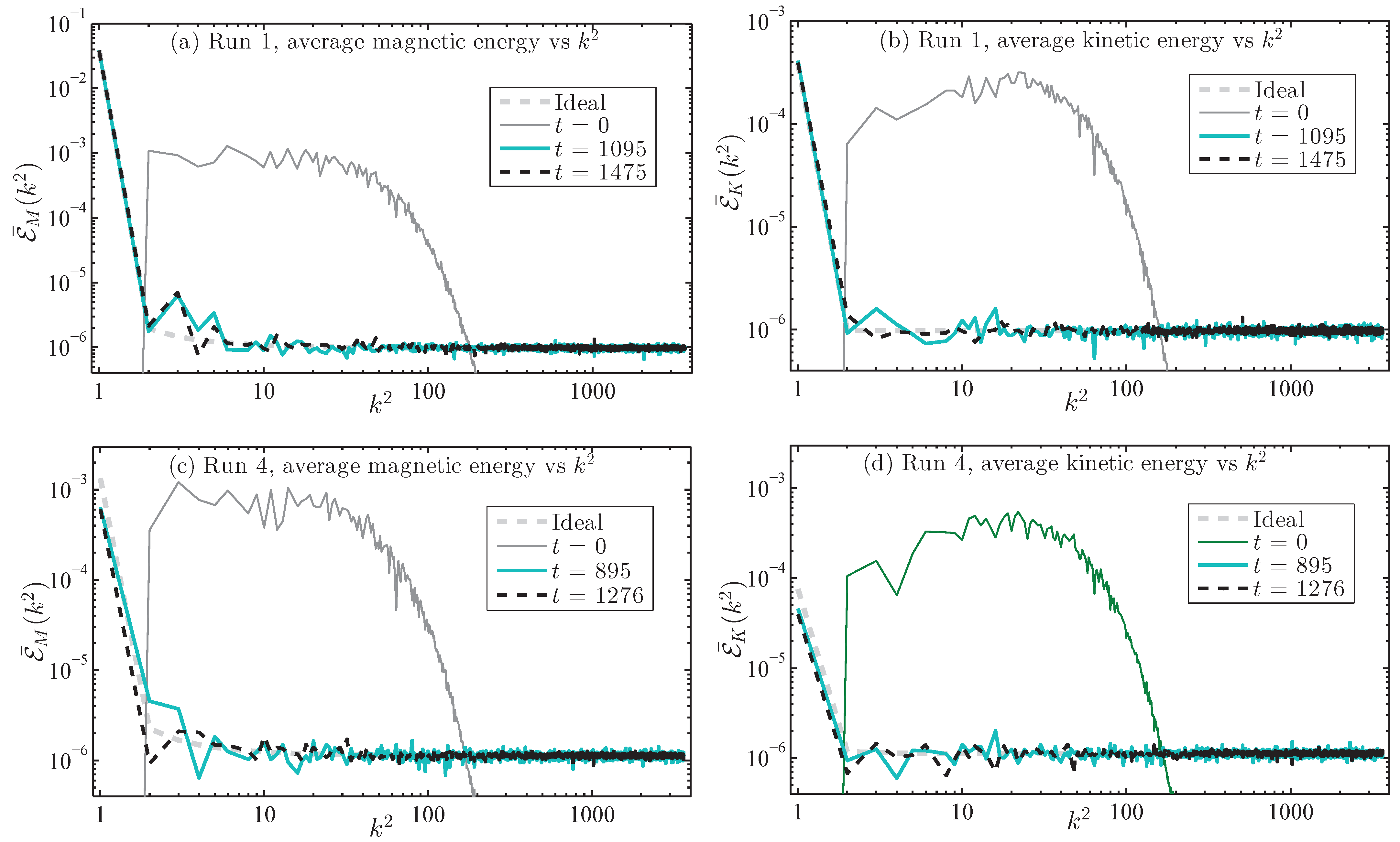
As seen in Table 1, the integral invariants of ideal MHD turbulence are the volume-averaged energy E and magnetic helicity when , as well as the cross-helicity when and when . In our numerical simulations, these ideal invariants typically have a standard deviation of less than 1% per million time-steps, while kinetic helicity , though an ideal invariant for hydrodynamic turbulence, falls to zero very quickly and then has small fluctuations about that value, as shown in Table 2. We stated that these runs came to ‘near equilibrium.’ To obtain an idea as to what this means, consider Figure 1 where we show, at different times for Runs 1 and 4, the average magnetic and kinetic energy spectra, and , for modes having the same value of . There are 3036 different values of , where , for ; the number of independent (i.e., but not ) is .
The definitions of the averaged spectra and are
Here, is the number of independent that satisfies . The number jumps around as increases; for example,
We have whenever ; see, for example, [31]. The full magnetic and kinetic energy spectra, and , jump wildly as increases, which is why we prefer to look at the average energy spectra (23) and (24), as in Figure 1. However, when averaged over nearest neighbors, is well approximated by and this can be used to give smoothed energy spectra, if desired.
Referring to [23], we find that the ideal expectation values of and are
Here, and , and are the normalized inverse temperatures related to inverse temperatures appearing in the phase space probability density; please see [13] for details. For each of the cases, , and are determined by numerically finding the minimum of the entropy functional with proviso that, for Case II (Runs 2a and 2b), ; for Case III (Run 3), ; and for Case V (Run 5), . The values of , and for the different runs are given in Table 3.
The spectra are shown in Figure 1 for various times. The spectra are approaching their expectation values and are near equilibrium; when they match the ideal expectation values (within small fluctuations), then they are in true equilibrium. The spectra and for Runs 3 and 5 will both be similar to those in Figure 1d, i.e., becoming flat, while the spectra for Runs 2a and 2b will be similar to Figure 1a,b, although not as highly peaked at .
Now, consider Figure 1, where average magnetic and kinetic energy spectra, and , for Runs 1 and 4 are given. These are averages over modes having the same value of ; there are 3036 different values of , where , for . In (a) and (b), the spectra are shown for times , 1095 and 1475 for Run 1 ( was the end of Run 1 in [13] and is the end of the continuation); and in (c) and (d) the spectra are shown for times , 895 and 1276 for Run 4 ( was the end of Run 4 in [13] and is the end of the continuation). The spectra in Figure 1 appear to be reaching expected values, although when MHD turbulence is in equilibrium, spectra will be seen to fluctuate about these ideal expectation values; moreover, for Run 4, an extra term may be needed in the perturbation expansion we used to more closely align computed and expected values at ; however, this effort will be deferred. The spectra for Runs 2a, 2b, 3 and 5 behave similarly. The correlation between computed and predicted spectra is another validation of the statistical theory.
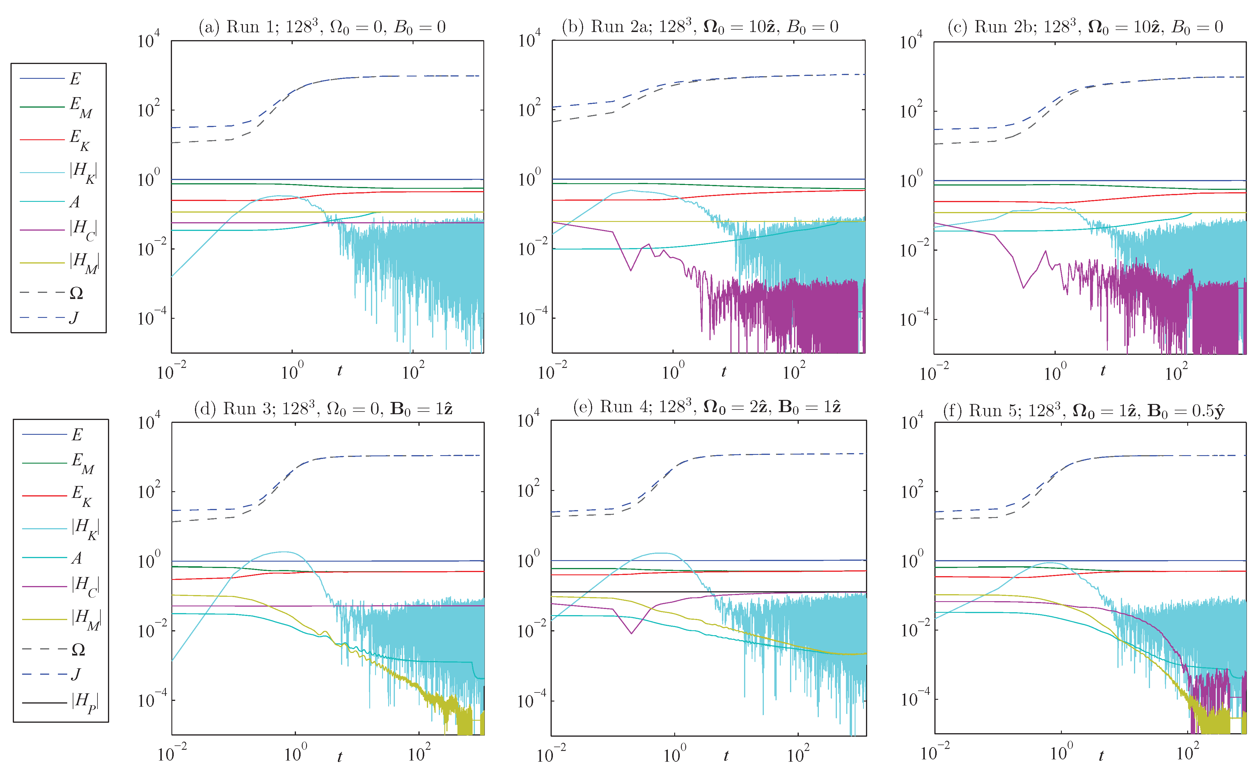
In Figure 2, we show how the six runs in Table 1 change over time with respect to volume-averaged energy E, magnetic energy , kinetic helicity , mean-squared magnetic vector potential A, cross helicity , magnetic helicity , enstrophy (mean-squared vorticity) and mean-squared electric current J; for Run 4, parallel helicity is also shown; again, please see (13)–(22) for precise definitions of these quantities. In Figure 2, the integral invariants for each run appear to be horizontal lines, i.e., have constant values. Time averages and standard deviations for these quantities over the course of the runs is given in Table 2. For each run in Table 2, the quantities that are supposed to be canonical invariants are again seen to be well conserved. The most conserved quantity, by far, is the magnetic helicity in Runs 1, 2a and 2b. Those quantities in Table 2 that have standard deviations larger in magnitude than their average values are basically just fluctuating around zero; in particular, this seems to be true for the kinetic helicity in every run except for Run 4, where it is part of the invariant parallel helicity . Also note that statistics for the enstrophy and mean-squared current J are essentially equal in each run, indicating that smaller length-scales effectively have equipartition in magnetic and kinetic energy.
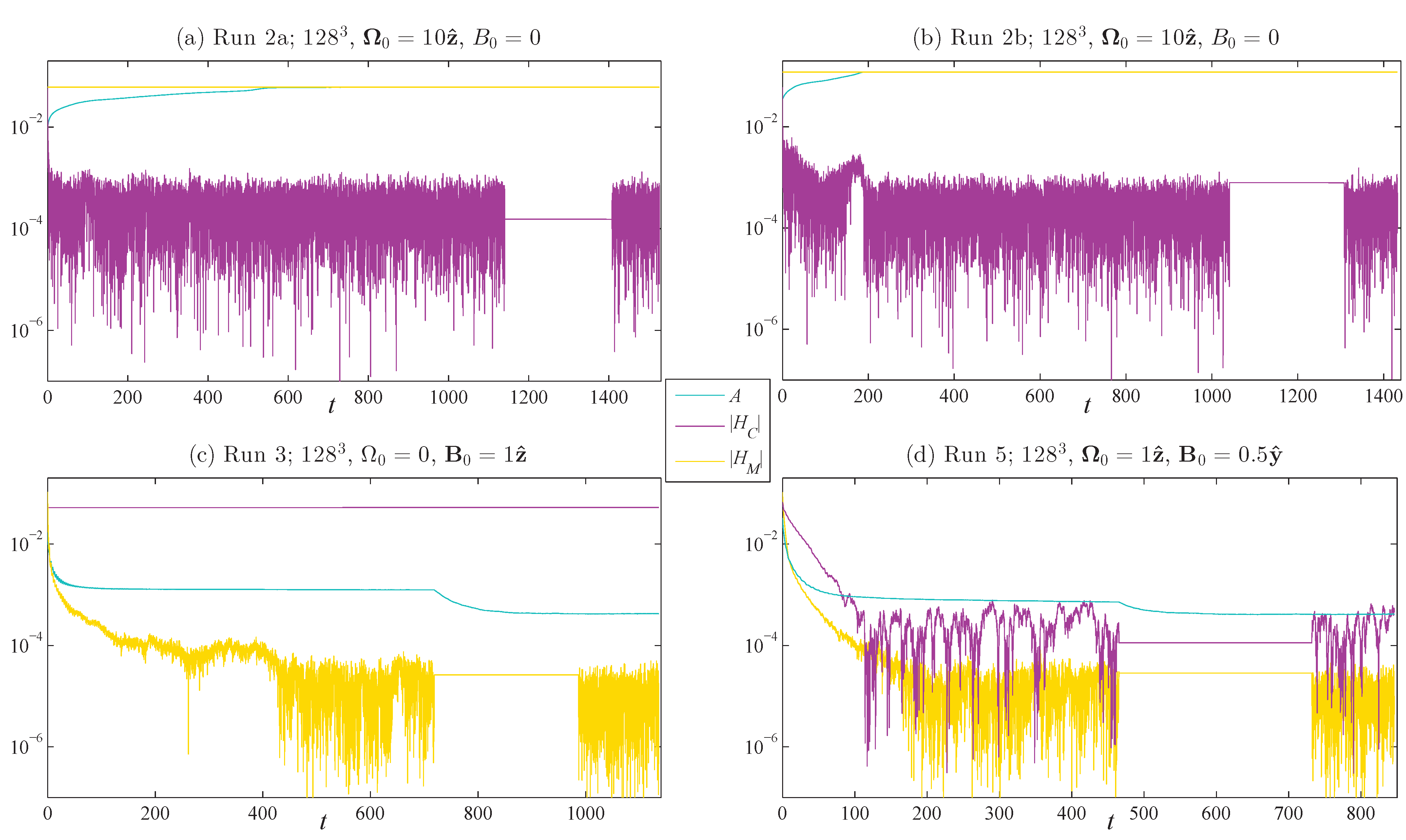
In Figure 2, near the ends of some runs, notice that one or both of the helicities and appear to become constants for a period of time. These helicities, as well as mean-average vector potential A for (a) Run 2a, (b) Run 2b, (c) Run 3 and (d) Run 5 are shown again in Figure 3. Here, we more clearly see that or or both become constant in these runs for a significant period of time: (a) (from to 1407.5); (b) (from to 1308.2); (c) (from to 986.9) and (d) (from to 732.0)—also notice that, during these periods in (c) and (d), A makes a transition to a lower value. The essential equivalence of the s is intriguing; however, to date, it remains unexplained and a puzzle for the future.
As mentioned earlier, continuation has resolved what seems to be an anomaly occurring in the transition phase, i.e., the appearance of mildly energetic coherent magnetic structures in Runs 3 and 5, as reported in [13]. These quasi-stationary structures are not predicted and, as we will see, eventually disappear, signaling the end of transition for those runs. Another novel feature is the behavior of the helicities and in those runs where one or both were not integral invariants. Specifically, this feature is that of the helicity or helicities that were not invariant became quasi-invariant for a significant interval of time and then resumed their fluctuating behavior. This happened in Runs 2a, 2b, 3 and 5, and signals the end of transition from initial conditions to equilibrium; for Runs 3 and 5, the quasi-invariance of the helicities coincided with the collapse of their transitory coherent structures, as seen in Figure 4.
In the previous work [13], there were many figures showing the trajectories of various complex Fourier coefficients as 2D phase plots (real vs. imaginary parts), but we will not look at these explicitly here. These 2D phase plots are quite interesting in that they are projections onto different complex planes of the random walk through a phase space of dimension 3,679,328 which the dynamical system takes as it evolves in time. These phase trajectories would not really look that different for the continued runs discussed here and the reader is referred back to [13] if there is a desire to view them. Here, we show behavior of the modes through 3D plots of a ‘dipole moment vector’, as described below.
For all the runs in Table 1, the values of all the and with were saved every 0.1 units of simulation time t (i.e., every 200 s). From these, we can calculate a time history of modal energies
We now define a ‘dipole moment vector’ as one that has components , , and an angle with respect to the z axis:
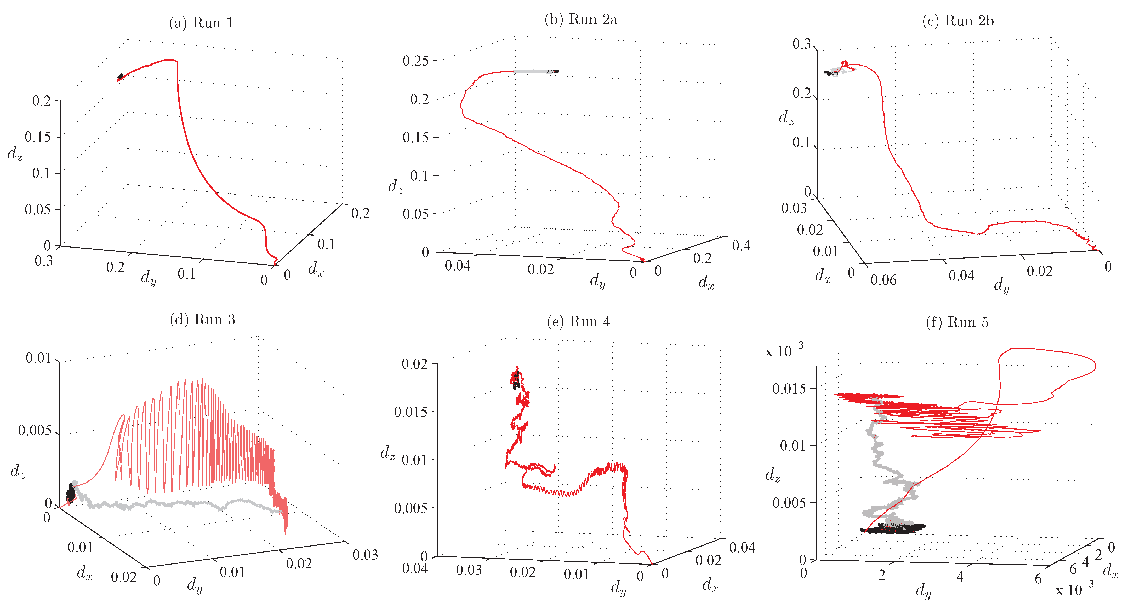
The evolution of is shown in Figure 4 for each of the runs in Table 1. In Figure 4, the initial growth of from is shown in red, while the last 10% of time for each run is shown in black; the periods shown in Figure 3 when or or both become constant appear in Figure 4 in gray for (b) Run 2a, (c) Run 2b, (d) Run 3 and (f) Run 5. Table 1 also has at the end of each run and there we see that Run 2a () and 2b () have vectors that are relatively well aligned with the rotation axis. We discuss how this happens in [13].
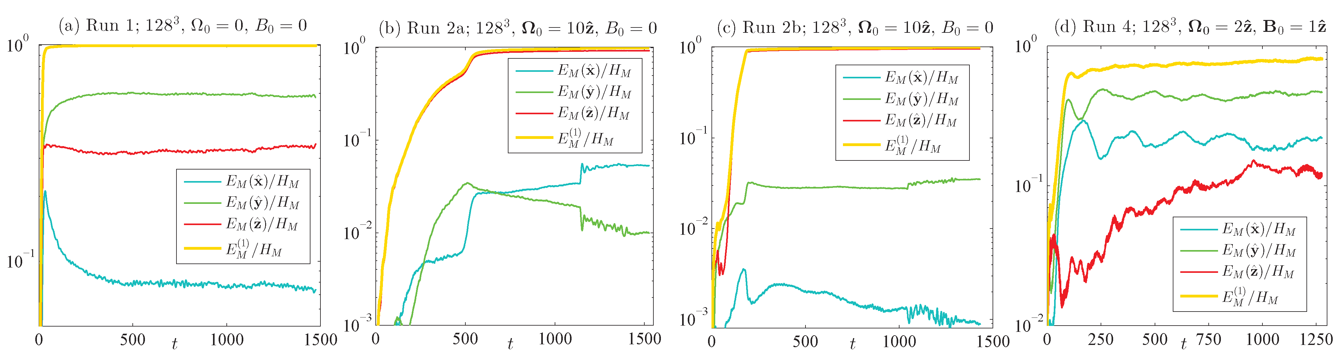
In Figure 5, the temporal evolution of the magnetic energies defined in (29) at , i.e., , , are presented for (a) Run 1, (b) Run 2a, (c) Run 2b and (d) Run 4. In Figure 4, the square roots of the defined a ‘dipole moment vector’ which was seen there to become quasi-stationary for these runs. In Figure 5, energies are divided by the corresponding mean values of over Runs 1, 2a and 2b, and the mean value of over the last 5% of Run 4. Here, we see a verification of the theoretical result that the energy of the dipole is , where, for the Fourier case, . This result is predicted for Runs 1, 2a and 2b, where is an ideal invariant, but also seems to apply approximately to Run 4, as seen in (d).
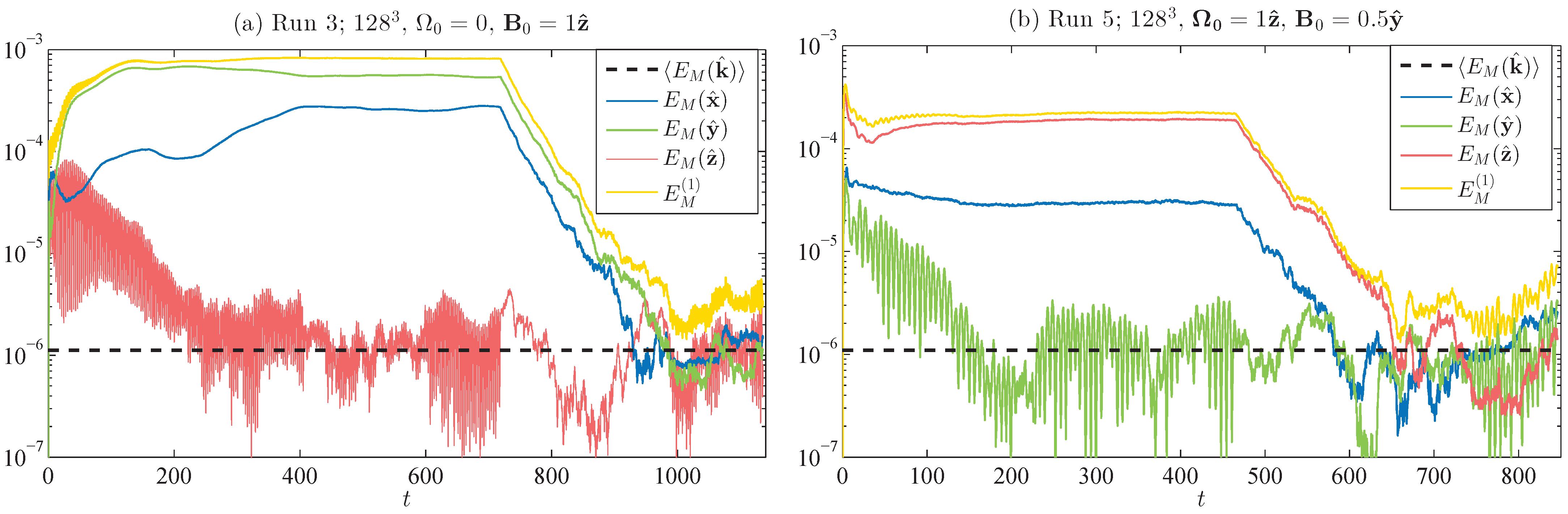
In Figure 6, the temporal evolution of the magnetic energies at , i.e., , , are presented for (a) Run 3 and (b) Run 5. The theoretical prediction when is not an invariant is that energy will be equipartioned among all Fourier modes and all and will have the same value, indicated above by . Here, we see that, during the initial phase of growth starting from the initial spectra shown in Figure 1, the temporary, relatively energetic, coherent structures arise but collapse in the final transition to equilibrium. This collapse occurs during the gray parts of the trajectories shown in Figure 4d,f. In Figure 6, we see that the fluctuate about their expectation values and that the anomalously large values that occurred during transition were, in fact, transitory.
5. Discussion
The results presented herein were found by continuing to run the simulations first presented in [13]. The continued runs have entered a state of apparent equilibrium and resolved an important open question from that work, specifically, we have seen that the coherent structures that appeared during transition from initial conditions in Runs 3 and 5—which had mean non-aligned magnetic fields—disappeared. Run 4, in which the mean magnetic field was aligned with the rotation axis, maintained a coherent structure, but one that was an order of magnitude less energetic that those in Runs 1, 2a and 2b, which had no mean magnetic field. Runs 1, 2a and 2b are the pertinent ones for modeling those planets and stars that contain a turbulent magnetofluid. The magnetic energy at (the ‘dipole’ energy ) matched the theoretical prediction that and that the effective ‘dipole moment vector’ , with dipole angle and defined in (30), was quasi-stationary, and, Runs 2a and 2b—which most closely modeled a rotating planetary core—showed alignment with the rotation axis, as seen in Table 2 and graphically illustrated in Figure 4. This quasi-stationarity was initially unsuspected [36] since the ensemble prediction is that all variables have zero-mean, so what we have seen, again, is a dynamically broken ergodicity.
Furthermore, the statistical theory of ideal MHD turbulence developed for a periodic box has the same form as that developed for a spherical shell [14]. Therein lies the importance of ideal results to the real MHD turbulence contained in planetary liquid cores and in the convective layers of stars: it is a basic, qualitative explanation of how these dipole magnetic fields arise and is thus a solution to ‘the dynamo problem.’ The statistical theory of ideal MHD turbulence began when [36] recognized that an inverse cascade of energy may move from intermediate scales to the largest scale in the system, as confirmed by [37]. After this initial discovery, it was eventually noticed in 1982 (as discussed in [13]) that this cascade created a coherent structure; the history of the subsequent development built on it is given in the list of related references appearing in [13]. Once it was realized that MHD turbulence, per se, was a dynamo, it was clear, at least to the author, that a deeper understanding of the statistical nature of ideal MHD turbulence, along with numerical simulations of real MHD turbulence [19,20], held the key to solving the ‘dynamo problem.’ That has been our path over many decades and it has led, we believe, to a fundamental understanding of self-generated planetary magnetic fields.
The exact nature of the turbulence within a planet, of course, is hidden from view in its deep interior, but observations of the global magnetic fields of the Earth and other planets indicate that they have long periods of quasi-stationarity in which a magnetic dipole field exists and is closely aligned with a rotation axis. The only requirements that we need to relate our results to these objects is for them to contain a sufficiently spherical shell of relatively incompressible, turbulent magnetofluid that is in a state of quasi-equilibrium, and that this state has an effectively constant (i.e., quasi-stationary) magnetic helicity; how this state is maintained is an important question, but extraneous to our simple (but not too simple) model. Our unique prediction that tells us that if a planet has a magnetic dipole field and we measure its value, then this also tells us that we know its magnetic helicity.
6. Conclusions
Although recent numerical simulations [13] of MHD turbulence corresponding to each of the five cases of ideal MHD turbulence in Table 1 had shown the quasi-stationary largest-scale coherent structure to arise during transition, once these runs were allowed to continue on and enter equilibrium, the transitory structures in Runs 3 and 5, where they were not predicted to exist, were seen to collapse. On the other hand, Runs 1, 2a and 2b had very energetic largest-scale coherent structures, both in transition and equilibrium, that were robust and behaved as predicted. Run 4, where the mean field and the rotation vector were parallel, also showed a coherent structure, although an order of magnitude less energetic. The largest-scale coherent structures seen in Runs 2a and 2b, in particular, represent the dipole magnetic fields that are seen to occur around various planets and stars.
The origin of these largest-scale coherent structures in ideal MHD turbulence has been understood through the application of classical statistical mechanics, with extensions, to the interacting set of Fourier coefficients; again, this is detailed in [13]. The difference between the statistical mechanics of an ideal gas and that of MHD turbulence, is that the former has only one invariant, the total energy, while the latter can have one or two invariant helicities. In the case of ideal MHD turbulence, an entropy functional can be defined and the minimization of this functional with respect to magnetic energy leads, through a series of logical steps, to an expression linking the energy of the dipole field to the magnetic helicity contained in the turbulent magnetofluid (as well as to a specific value for the phase entropy). Thus, in dynamo theory, as we have presented it, the statistical mechanics of ideal MHD turbulence plays an essential role and is a key to theoretical understanding of the geodynamo, as well as other planetary and stellar dynamos. Numerical simulation is also another key factor as it offers a validation of the statistical theory.
In this paper, we presented new computational data, discussed new results and resolved an open question left over from previous work. The importance of our theoretical and numerical results, both now and in the past [13], is that they show that MHD turbulence, per se, is a dynamo that produces an energetic, quasi-steady, magnetic dipole that is closely aligned with a rotation axis when one is present. The energy in the ‘dipole’ field and magnetic helicity were predicted and seen to satisfy Equation (1), the fundamental relation . This relation is also a prediction for model systems in which a turbulent magnetofluid is confined within a spherical shell, since ideal MHD turbulence in this geometry has the same statistical mechanics as in the Fourier case. In summary, broken ergodicity in MHD turbulence appears to be a viable solution to the ‘dynamo problem.’
A future direction that our investigations can take is to add dissipation and forcing to our simulations as was previously performed on grids [19,20]; we also wish to move to the larger grid-sizes enabled by massively parallel processing. The methods employed to force a model magnetofluid at intermediate wavenumbers are speculative because physical forcing mechanisms are hidden from observation within a planet or star. Nevertheless, having used a variety of mid-wavenumber, helical forcing methods on grids [19,20], we have always seen behavior analogous to the ideal MHD turbulence at the largest-length scale, specifically the emergence of a largest-scale coherent magnetic structure whose energy is determined by the amount of magnetic helicity contained by the magnetofluid turbulence in those cases (I and II) that are most pertinent to planets and stars. We would expect to see this in and greater grid-size simulations that were dissipative and forced. Perhaps some novel effects would also occur, but this, and much else, remains worked that is yet to be performed.
Funding
This research received no external funding.
Data Availability Statement
Data is available from author.
Acknowledgments
This research did not receive any specific grant from funding agencies in the public, commercial, or not-for-profit sectors.
Conflicts of Interest
The author declares no conflict of interest.
References
- Larmor, J. How could a rotating body such as the sun become a magnet? In Proceedings of the Report of the 87th Meeting of the British Association for the Advancement of Science, Poole, UK, 9–13 September 1919; John Murray: London, UK, 1920; pp. 159–160. [Google Scholar]
- Elsasser, W.M. Hydromagnetic dynamo theory. Rev. Mod. Phys. 1956, 28, 135–163. [Google Scholar] [CrossRef]
- Alken, P.; Thébault, E.; Beggan, C.D.; Amit, H.; Aubert, J.; Baerenzung, J.; Bondar, T.N.; Brown, W.J.; Califf, S.; Chambodut, A.; et al. International Geomagnetic Reference Field: The 13th generation. Earth Planets Space 2021, 73, 49. [Google Scholar] [CrossRef]
- Nataf, H.-C.; Schaeffer, N. Turbulence in the Core. In Treatise on Geophysics 8: Core Dynamics, 2nd ed.; Olson, P., Ed.; Elsevier: Amsterdam, The Netherlands, 2015; pp. 161–181. [Google Scholar]
- Glatzmaier, G.A.; Roberts, P.H. A three-dimensional self-consistent computer simulation of a geomagnetic field reversal. Nature 1995, 377, 203–209. [Google Scholar] [CrossRef]
- Glatzmaier, G.A.; Roberts, P.H. A three-dimensional convective dynamo solution with rotating and finitely conducting inner core and mantle. Phys. Earth Planet. Int. 1995, 91, 63–75. [Google Scholar] [CrossRef]
- Kuang, W.; Bloxham, J. An Earth-like numerical dynamo model. Nature 1997, 389, 371–374. [Google Scholar] [CrossRef]
- Le Bars, M.; Barik, A.; Burmann, F.; Lathrop, D.P.; Noir, J.; Schaeffer, N.; Triana, S.A. Fluid Dynamics Experiments for Planetary Interiors. Surv. Geophys. 2022, 43, 229–261. [Google Scholar] [CrossRef]
- Gailitis, A.; Lielausis, O.; Platacis, E.; Demenťev, S.; Cifersons, A.; Gerbeth, G.; Gundrum, T.; Stefani, F.; Christen, M.; Will, G. Magnetic field saturation in the Riga dynamo experiment. Phys. Rev. Lett. 2001, 86, 3024–3027. [Google Scholar] [CrossRef] [Green Version]
- Monchaux, R.; Berhanu, M.; Bourgoin, M.; Moulin, M.; Odier, P.; Pinton, J.F.; Volk, R.; Fauve, S.; Mordant, N.; Pétrélis, F.; et al. Generation of a Magnetic Field by Dynamo Action in a Turbulent Flow of Liquid Sodium. Phys. Rev. Lett. 2007, 98, 044502. [Google Scholar] [CrossRef] [Green Version]
- Stieglitz, R.; Muüller, U. Experimental demonstration of a homogeneous two-scale dynamo. Phys. Fluids 2002, 13, 561–564. [Google Scholar] [CrossRef]
- Davidson, P.A. Turbulence in Rotating and Electrically Conducting Fluids; Cambridge U.P.: Cambridge, UK, 2013; p. 532. [Google Scholar]
- Shebalin, J.V. Transition to Equilibrium and Coherent Structure in Ideal MHD Turbulence. Fluids 2023, 8, 107. [Google Scholar] [CrossRef]
- Shebalin, J.V. Broken ergodicity, magnetic helicity, and the MHD dynamo. Geophys. Astrophys. Fluid Dyn. 2013, 107, 353–375. [Google Scholar] [CrossRef]
- Etchevest, M.; Fontana, M.; Dmitruk, P. Behavior of hydrodynamic and magnetohydrodynamic turbulence in a rotating sphere with precession and dynamo action. Phys. Rev. Fluids 2022, 7, 103801. [Google Scholar] [CrossRef]
- Mininni, P.D.; Montgomery, D. Magnetohydrodynamic activity inside a sphere. Phys. Fluids 2006, 18, 116602. [Google Scholar] [CrossRef] [Green Version]
- Mininni, P.D.; Montgomery, D.; Turner, L. Hydrodynamic and magnetohydrodynamic computations inside a rotating sphere. New J. Phys. 2007, 9, 303–330. [Google Scholar] [CrossRef]
- Palmer, R.G. Broken ergodicity. Adv. Phys. 1982, 31, 669–735. [Google Scholar] [CrossRef]
- Shebalin, J.V. Magnetohydrodynamic turbulence and the geodynamo. Phys. Earth Planet. Int. 2018, 285, 59–75. [Google Scholar] [CrossRef] [Green Version]
- Shebalin, J.V. Magnetic Helicity and the Geodynamo. Fluids 2021, 6, 99. [Google Scholar] [CrossRef]
- Lee, T.D. On some statistical properties of Hydrodynamical and magneto-hydrodynamical fields. Q. Appl. Math. 1952, 10, 69–74. [Google Scholar] [CrossRef] [Green Version]
- Woltjer, L. A theorem on force-free magnetic fields. Proc. Nat. Acad. Sci. USA 1958, 44, 489–491. [Google Scholar] [CrossRef] [Green Version]
- Shebalin, J.V. Broken ergodicity in magnetohydrodynamic turbulence. Geophys. Astrophys. Fluid Dyn. 2013, 107, 411–466. [Google Scholar] [CrossRef]
- Galtier, S. Weak turbulence theory for rotating magnetohydrodynamics and planetary flows. J. Fluid Mech. 2014, 757, 114–154. [Google Scholar] [CrossRef] [Green Version]
- Rice, J.E. Experimental observations of driven and intrinsic rotation in tokamak plasmas. Plasma Phys. Control. Fusion 2016, 58, 083001. [Google Scholar] [CrossRef]
- Kraichnan, R.H. Helical turbulence and absolute equilibrium. J. Fluid Mech. 1973, 59, 745–752. [Google Scholar] [CrossRef]
- Orszag, S.A.; Patterson, G.S. Numerical simulation of three-dimensional homogeneous isotropic turbulence. Phys. Rev. Lett. 1972, 28, 76–79. [Google Scholar] [CrossRef]
- Gazdag, J. Time-differencing schemes and transform methods. J. Comp. Phys. 1976, 20, 196–207. [Google Scholar] [CrossRef]
- Verma, M.; Sharma, M.; Chatterjee, S.; Alam, S. Variable Energy Fluxes and Exact Relations in Magnetohydrodynamics Turbulence. Fluids 2021, 6, 225. [Google Scholar] [CrossRef]
- Chatterjee, A.G.; Verma, M.K.; Kumar, A.; Samtaney, R.; Hadri, B.; Khurram, R. Scaling of a Fast Fourier Transform and a pseudo-spectral fluid solver up to 196608 cores. J. Parallel Distrib. Comput. 2018, 113, 77–91. [Google Scholar] [CrossRef] [Green Version]
- Andrews, G.E. Number Theory; Dover Pubs.: New York, NY, USA, 1994; p. 148. [Google Scholar]
- Goldreich, P.; Sridhar, S. Toward a theory of interstellar turbulence. 2: Strong alfvenic turbulence. Astrophys. J. 1995, 438, 763–775. [Google Scholar] [CrossRef]
- Goldreich, P.; Sridhar, S. Magnetohydrodynamic Turbulence Revisited. Astrophys. J. 1995, 485, 680–688. [Google Scholar] [CrossRef] [Green Version]
- Oughton, S.; Priest, E.R.; Matthaeus, W.H. The influence of a mean magnetic field on three-dimensional magnetohydrodynamic turbulence. J. Fluid Mech. 1994, 280, 95–117. [Google Scholar] [CrossRef] [Green Version]
- Shebalin, J.V.; Matthaeus, W.H.; Montgomery, D. Anisotropy in MHD turbulence due to a mean magnetic field. J. Plasma Phys. 1983, 29, 525–547. [Google Scholar] [CrossRef] [Green Version]
- Frisch, U.; Pouquet, A.; Leorat, J.; Mazure, A. Possibility of an inverse cascade of magnetic helicity in magnetohydrodynamic turbulence. J. Fluid Mech. 1975, 68, 769–778. [Google Scholar] [CrossRef] [Green Version]
- Pouquet, A.; Patterson, G.S. Numerical simulation of helical magnetohydrodynamic turbulence. J. Fluid Mech. 1978, 85, 305–323. [Google Scholar] [CrossRef]
Figure 1.
(Color online) Average magnetic and kinetic energy spectra, and , for Runs 1 and 4. These are averages over modes having the same value of ; there are 3036 different values of , where , for . Spectra are shown in (a,b) for times , 1095 and 1475 for Run 1, and in (c,d) for times , 895 and 1276 for Run 4. As seen here, spectra are expected to fluctuate about ideal expectation values.

Figure 2.
(Color online) Here, we see volume-averages defined in (13)–(22). Those quantities that are supposed to be canonical invariants are, in fact, constant in each run: (a) Run 1: E, and ; (b) Run 2a: E and ; (c) Run 2b: E and ; (d) Run 3: E and ; (e) Run 4: E and ; and (f) Run 5: only E. Note that there are periods of quasi-stationarity near the ends of (b) Run 2a, (c) Run 2b, (d) Run 3 and (f) Run 5; these will be examined more closely in Figure 3. Note also that the absolute value of kinetic helicity is similar in all runs in that it merely fluctuates around zero, signifying that is not of fundamental importance in MHD turbulence.

Figure 3.
(Color online) Absolute values of helicities and , as well as mean-average vector potential A for (a) Run 2a, (b) Run 2b, (c) Run 3 and (d) Run 5. Notice how or or both become constant in these runs for a short period of time: (a) , (b) , (c) and (d) ; also notice that during these periods in (c,d), the mean-squared vector potential A, defined by (17), makes a transition to a lower value.

Figure 4.
(Color online) The 3D ‘dipole moment vector’ is defined by , and and its evolution during each of the six runs is shown here. The initial growth of , starting from when it is very close to the origin, is shown in red; at the end of each trajectory, the last 10% of the run time is shown in black. The periods in Figure 3 when or or both become constant are shown in gray for (b) Run 2a, (c) Run 2b, (d) Run 3 and (f) Run 5; during these periods in (d,f), the temporary coherent structure represented by collapses The runs shown in (a–c,e) do not collapse but represent coherent structures.

Figure 5.
(Color online) The evolution of magnetic energies at , i.e., , , are presented for (a) Run 1, (b) Run 2a, (c) Run 2b and (d) Run 4. In Figure 4, the square roots of the defined a ‘dipole moment vector’ which was seen there to become quasi-stationary for these runs. Here, the energies are normalized by the mean value of during Runs 1, 2a and 2b, and the mean value of over the last 5% of Run 4. We see a verification of the fundamental theoretical result (1) that the energy of the dipole is , where, for the Fourier case, . This result is predicted for Runs 1, 2a and 2b, where is an ideal invariant, but also seems to apply approximately to Run 4, as seen in (d).

Figure 6.
(Color online) The evolution of the magnetic energies at , i.e., , , are shown for (a) Run 3 and (b) Run 5. The theoretical prediction when is not an invariant is that energy will be equipartioned among all Fourier modes and all and , defined in (28) and (29), will have the same expectation value . During the initial phase of growth, relatively energetic, coherent structures arise but then collapse in the final transition to equilibrium. This collapse occurs during the gray parts of the trajectories shown in Figure 4d,f.


Table 1.
Cases and associated runs with different integral invariants for ideal MHD turbulence. When , the ‘parallel helicity’ of Case IV is .
Table 1.
Cases and associated runs with different integral invariants for ideal MHD turbulence. When , the ‘parallel helicity’ of Case IV is .
| Case | Mean Field | Rotation | Invariants | Runs |
|---|---|---|---|---|
| I | E, , | 1 | ||
| II | E, | 2a,b | ||
| III | E, | 3 | ||
| IV | E, | 4 | ||
| V | E | 5 |
Table 2.
Time averages (avg) and standard deviations (std) for global quantities over the last quarter of each run appear below for six new ideal MHD turbulence long-time Runs 1, 2a, 2b, 3, 4 and 5. The global quantities are: energy E, kinetic energy , magnetic energy , mean-squared vector potential A, kinetic helicity , magnetic helicity , cross helicity , parallel helicity , enstrophy and mean-squared current J; these are defined in (2)–(4) and more explicitly in (13)–(22). The angle at , is defined in (30) and is analogous to the geomagnetic dipole angle (if all dipole moment components were equal, then ).
| Run: | 1 | 2a | 2b | 3 | 4 | 5 |
|---|---|---|---|---|---|---|
| : | 1475 | 1526 | 1426 | 1132 | 1276 | 846 |
| 0 | 0 | |||||
| 0 | 0 | 0 | ||||
| 1.01100 | 1.01246 | 1.01226 | 1.02980 | 1.03506 | 1.00699 | |
| 1.2609 × 10 | 1.1801 × 10 | 1.2758 × 10 | 2.1086 × 10 | 1.7358 × 10 | 7.7732 × 10 | |
| 0.44822 | 0.47564 | 0.44539 | 0.51489 | 0.51648 | 0.50349 | |
| 6.8596 × 10 | 8.3465 × 10 | 9.4303 × 10 | 1.1379 × 10 | 9.1951 × 10 | 5.0655 × 10 | |
| 0.56277 | 0.53665 | 0.56648 | 0.51490 | 0.51961 | 0.50350 | |
| 0.56278 | 0.53682 | 0.56687 | 0.51491 | 0.51857 | 0.50350 | |
| 7.0116 × 10 | 5.4670 × 10 | 5.1064 × 10 | 1.0846 × 10 | 9.4653 × 10 | 5.0999 × 10 | |
| 1.1570 | 6.0735 × 10 | 1.2060 | 4.5031 × 10 | 2.1962 × 10 | 4.1079 × 10 | |
| 6.6740 | 1.2467 × 10 | 1.9983 × 10 | 5.9076 × 10 | 3.5112 × 10 | 5.2188 | |
| 6.0009 × 10 | −4.1736 × 10 | −6.2487 × 10 | 3.5946 × 10 | 3.2657 × 10 | −5.2689 × 10 | |
| 2.1744 × 10 | 2.3103 × 10 | 2.1481 × 10 | 2.5246 × 10 | 2.4646 × 10 | 2.3873 × 10 | |
| 1.1570 | 6.0840 × 10 | 1.2070 | −1.5986 × 10 | 2.2020 × 10 | −1.6685 × 10 | |
| 2.4011 | 2.3803 | 5.7460 | 1.5901 × 10 | 3.5315 × 10 | 1.7279 × 10 | |
| 5.6359 × 10 | −9.9448 × 10 | 4.5145 × 10 | 5.2491 × 10 | −1.2703 | −1.0241 × 10 | |
| 6.5119 × 10 | 2.5384 × 10 | 4.5670 × 10 | 2.1550 × 10 | 6.9637 × 10 | 1.7423 × 10 | |
| ⋯ | ⋯ | ⋯ | ⋯ | −1.3144 | ⋯ | |
| ⋯ | ⋯ | ⋯ | ⋯ | 5.2471 × 10 | ⋯ | |
| 9.7631 × 10 | 1.0387 × 10 | 9.7270 × 10 | 1.1245 × 10 | 1.1277 × 10 | 1.0996 × 10 | |
| 1.5758 | 1.9354 | 2.0917 | 2.5683 | 2.0880 | 1.2396 | |
| 9.7686 × 10 | 1.0393 × 10 | 9.7328 × 10 | 1.1244 × 10 | 1.1282 × 10 | 1.0996 × 10 | |
| 1.5981 | 1.9306 | 2.1060 | 2.5085 | 2.0831 | 1.2747 |
Table 3.
Values of the inverse temperatures , and for the Runs in Table 1 with proviso that, for Runs 2a and 2b, ; for Run 3, ; and for Run 5, and . When needed, , and took their values from , and , respectively, in Table 2 (the need for precision here is due to the possible smallness of the denominators in (26) and (27)).
| Run | |||
|---|---|---|---|
| 1 | 0.99101483544 | ||
| 2a | 0.92181618056 | 0 | |
| 2b | 0.98391439550 | 0 | |
| 3 | 0.83658011283 | 0 | |
| 4 | 0.90153576833 | 0.42548700154 | |
| 5 | 0.87722015381 | 0 | 0 |
Disclaimer/Publisher’s Note: The statements, opinions and data contained in all publications are solely those of the individual author(s) and contributor(s) and not of MDPI and/or the editor(s). MDPI and/or the editor(s) disclaim responsibility for any injury to people or property resulting from any ideas, methods, instructions or products referred to in the content. |
© 2023 by the author. Licensee MDPI, Basel, Switzerland. This article is an open access article distributed under the terms and conditions of the Creative Commons Attribution (CC BY) license (https://creativecommons.org/licenses/by/4.0/).
Share and Cite
MDPI and ACS Style
Shebalin, J.V. Transition to Equilibrium and Coherent Structure in Ideal MHD Turbulence, Part 2. Fluids 2023, 8, 181. https://doi.org/10.3390/fluids8060181
AMA Style
Shebalin JV. Transition to Equilibrium and Coherent Structure in Ideal MHD Turbulence, Part 2. Fluids. 2023; 8(6):181. https://doi.org/10.3390/fluids8060181
Chicago/Turabian StyleShebalin, John V. 2023. "Transition to Equilibrium and Coherent Structure in Ideal MHD Turbulence, Part 2" Fluids 8, no. 6: 181. https://doi.org/10.3390/fluids8060181