
Second-Order Time-Accurate ALE Schemes for Flow Computations with Moving and Topologically Changing Grids

Abstract
:1. Introduction
1.1. Motivation of This Research
1.2. Goals and Highlights
1.3. Paper Structure
2. Governing Equations for Fluid Transport in Time-Varying Domains
3. Variable Positioning and Spatial Discretization
- -
- Diffusive term (Laplacian) of a quantity , e.g., :where is the surface normal gradient of . The subscript f in (4) indicates the cell-to-face interpolated quantities. Linear cell-to-face interpolation was applied: for irregular polyhedral meshes, interpolation is generalized by defining a weight w for each face:where is the face-interpolated quantity. Subscripts P and N indicate values at the centers of two neighboring cells. The surface gradient of a quantity is decomposed into an orthogonal part and a (non-orthogonal) correction:where and are the uncorrected normal gradient from the two values of the two cells sharing the face. The explicit part is computed from (5) as:where in this work; the normal gradient is computed as:
- -
- Gradient terms: these were discretized by the Green–Gauss theorem:where is the volume of the polyhedral cell P, and is the surface vector of the f-th face of the cell.
- -
- Non-linear terms (convective terms): the convective term in the momentum balance is linearized with the Picard approach: the mass flux is treated explicitly, and the non-linear term is approximated by:the index in (10) denotes that the values are taken from the result of the previous time step. A technique for momentum-based interpolation of mass fluxes on cell faces [38] is used to mimic staggered-grid discretization to prevent checkerboard effects. Using the divergence theorem, the convective terms are rewritten as:The velocity is interpolated with the same approach presented in (5), while a second-order central differencing scheme is used for the fluxes.
- -
- Conservative remap: in a dynamic grid, the position of the cell centers changes from one time step to the next. Linear interpolation is used for mapping cell-centered quantities from the old to the new mesh, to favor the convergence rate of the solver:However, remapping of the fields defined over the faces of the CVs cannot be applied to extensive quantities, as it strongly influences the conservation (and the convergence rate) of the p-U algorithm. To ensure conservation, fields in the CV faces are interpolated from the values in the CV centers, and a Helmholtz-like equation is then solved to ensure that the remapped state is fully conservative.
4. Finite Volume ALE Scheme for Dynamic Meshes with Topology Changes
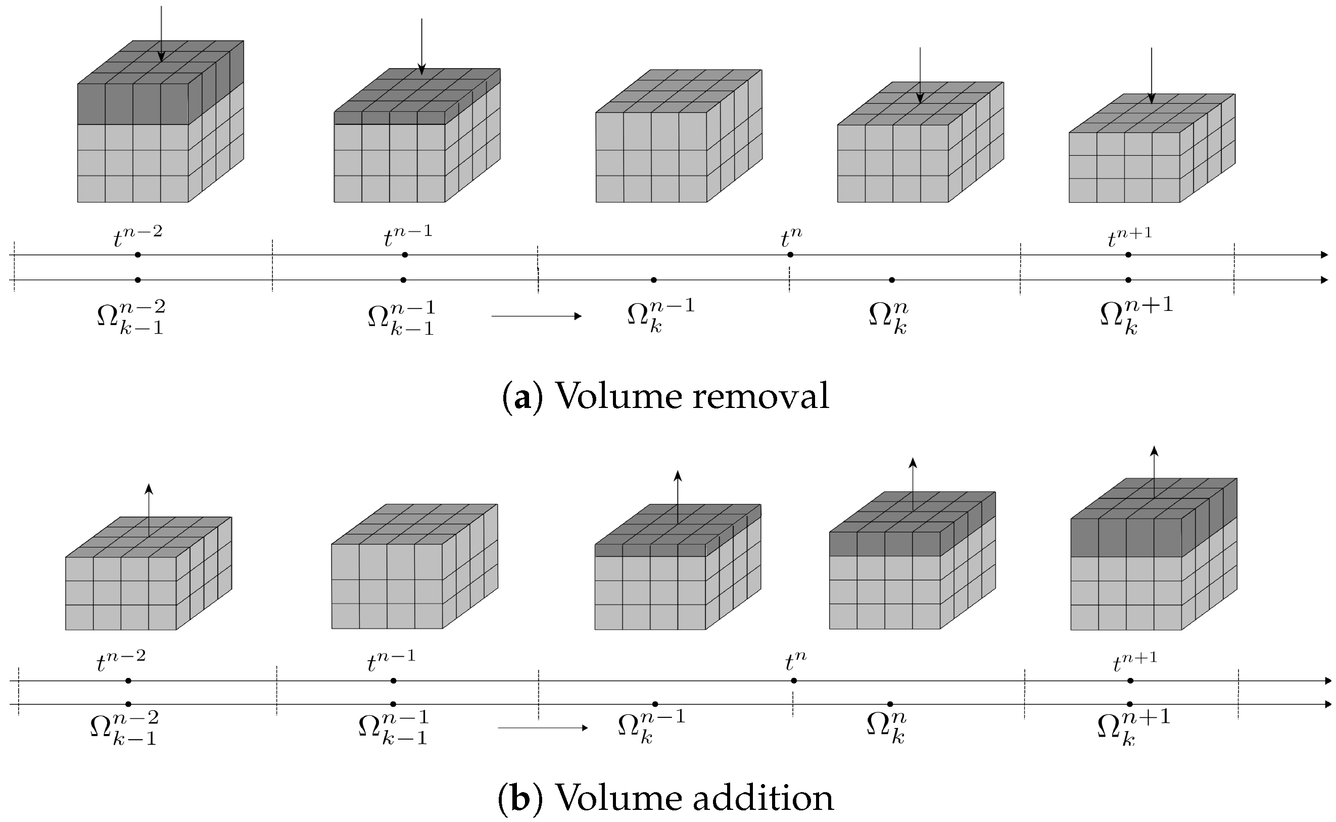
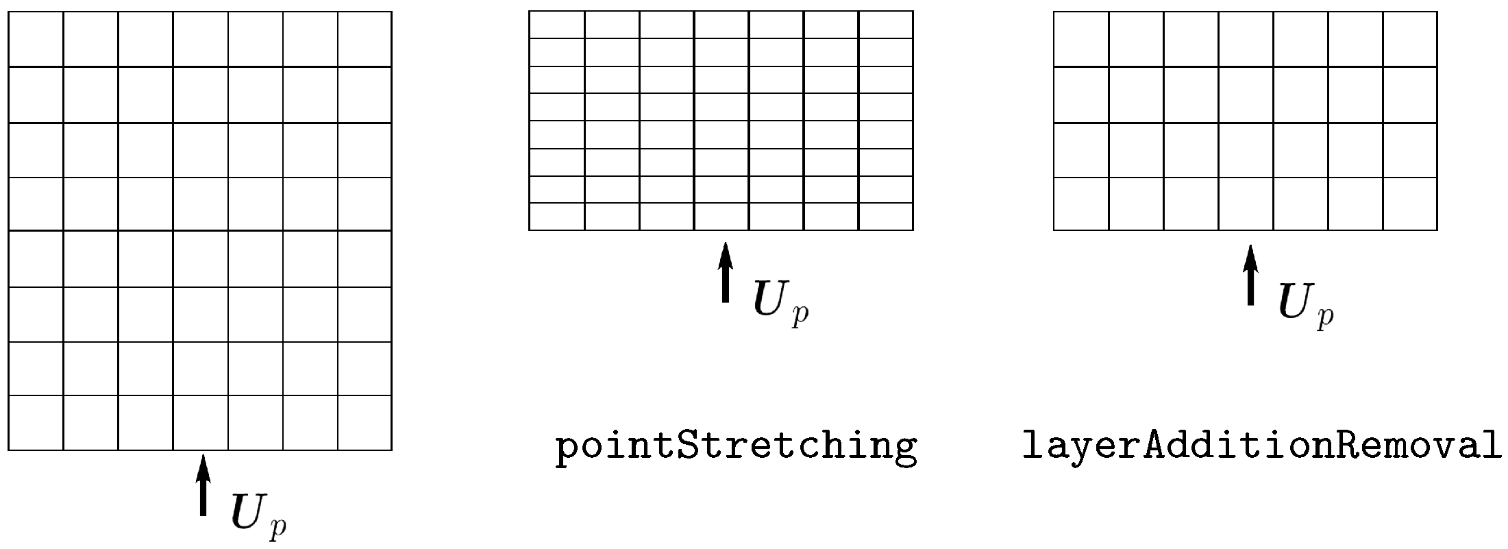
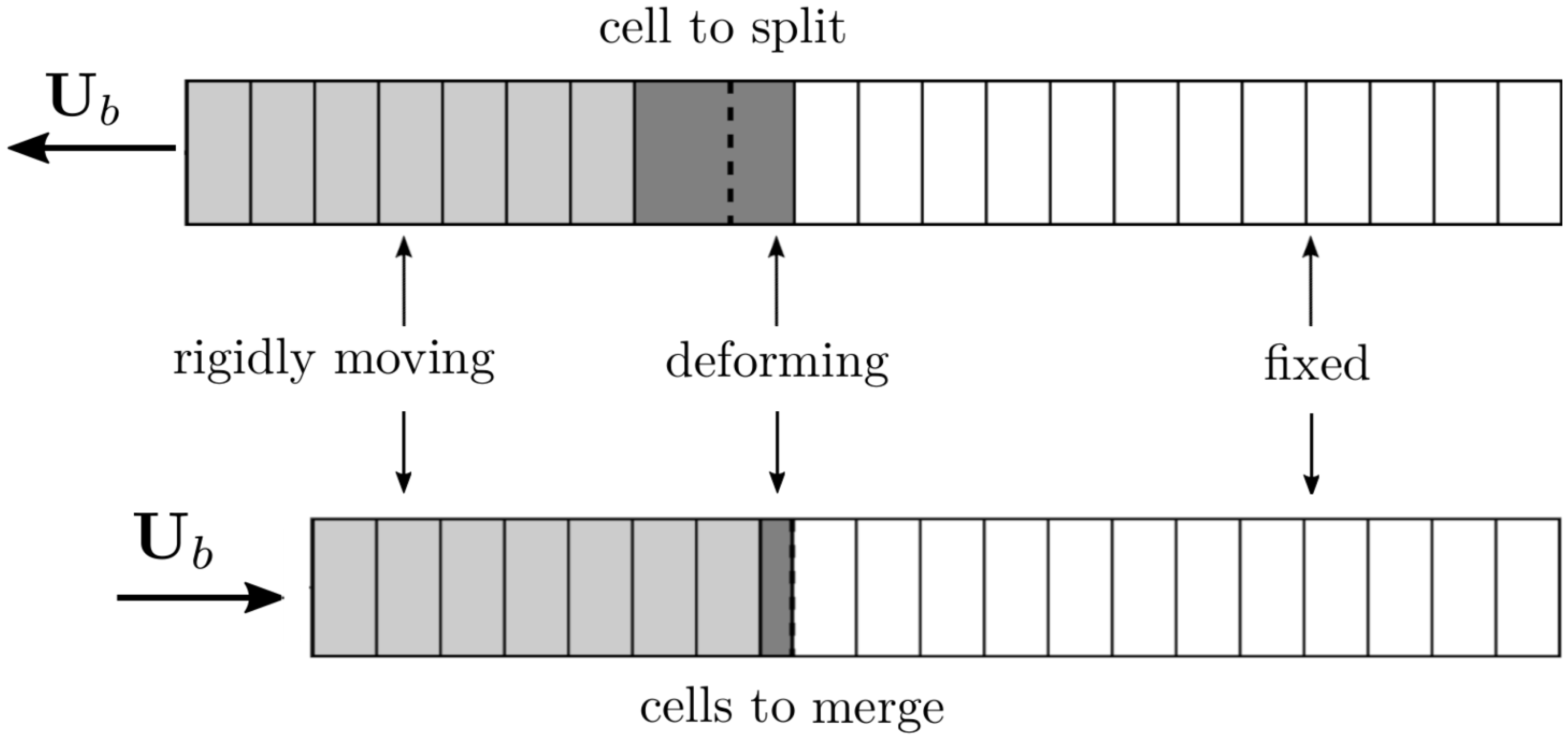
5. Temporal Discretization with Topology Changes
- -
- With cell inflation: it is assumed that the cell faces at are duplicated to generate new zero-volume cells, which are then inflated to form the new cells at :and the local topology change (volume addition and mesh motion) is accounted for by the mesh fluxes of the newly added faces from position , which are computed as:where is the mesh flux corresponding to the volume swept by each face from state to state .
- -
- Without cell inflation: if the newly added faces are assumed to be inserted into their final positions at state , their mesh fluxes will be zero:and the local topology change will be accounted for in the equation by a conservative remapping of the cell quantities between two different grids. The same reasoning can be applied if a static face is being removed.
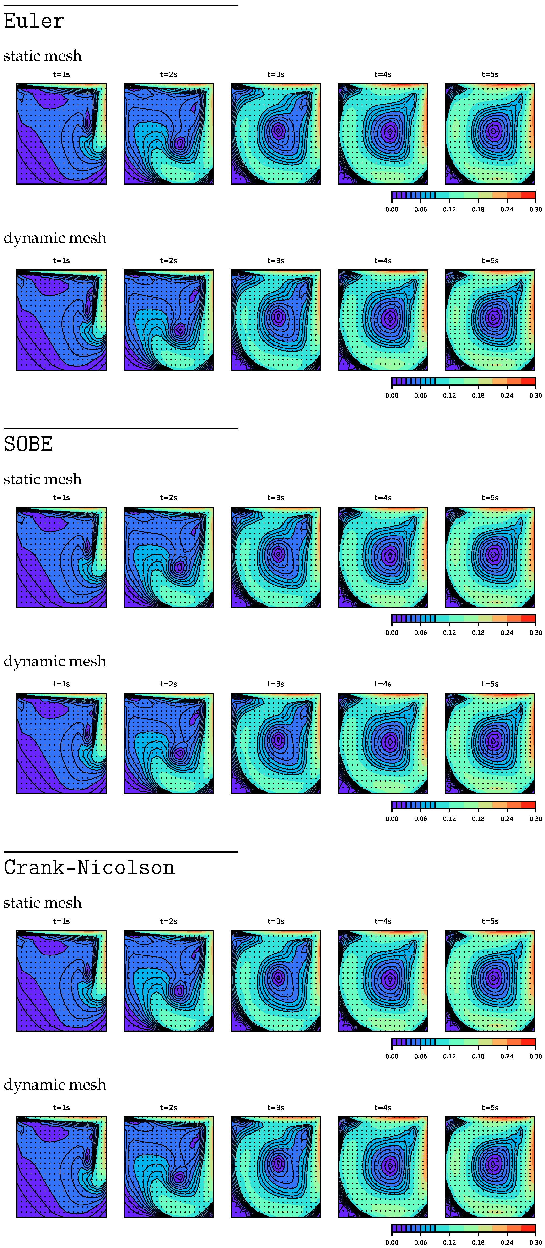
6. Second-Order Temporal Discretization with Dynamic Mesh Refinement
6.1. Second-Order Backward Euler Scheme (SOBE)
6.2. Crank–Nicolson Time-Differencing Scheme (CN)
6.3. Adaptive Mesh Refinement
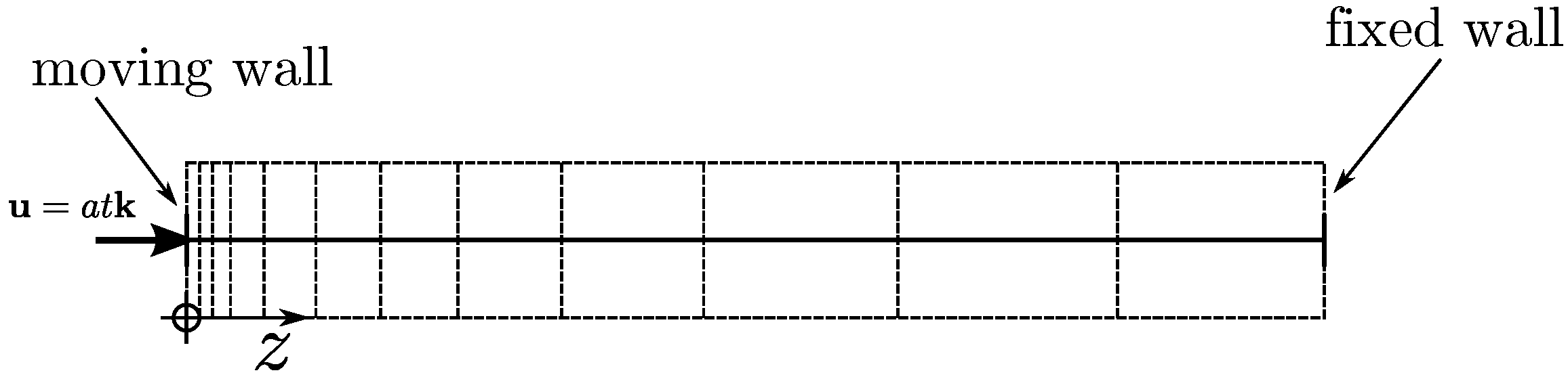
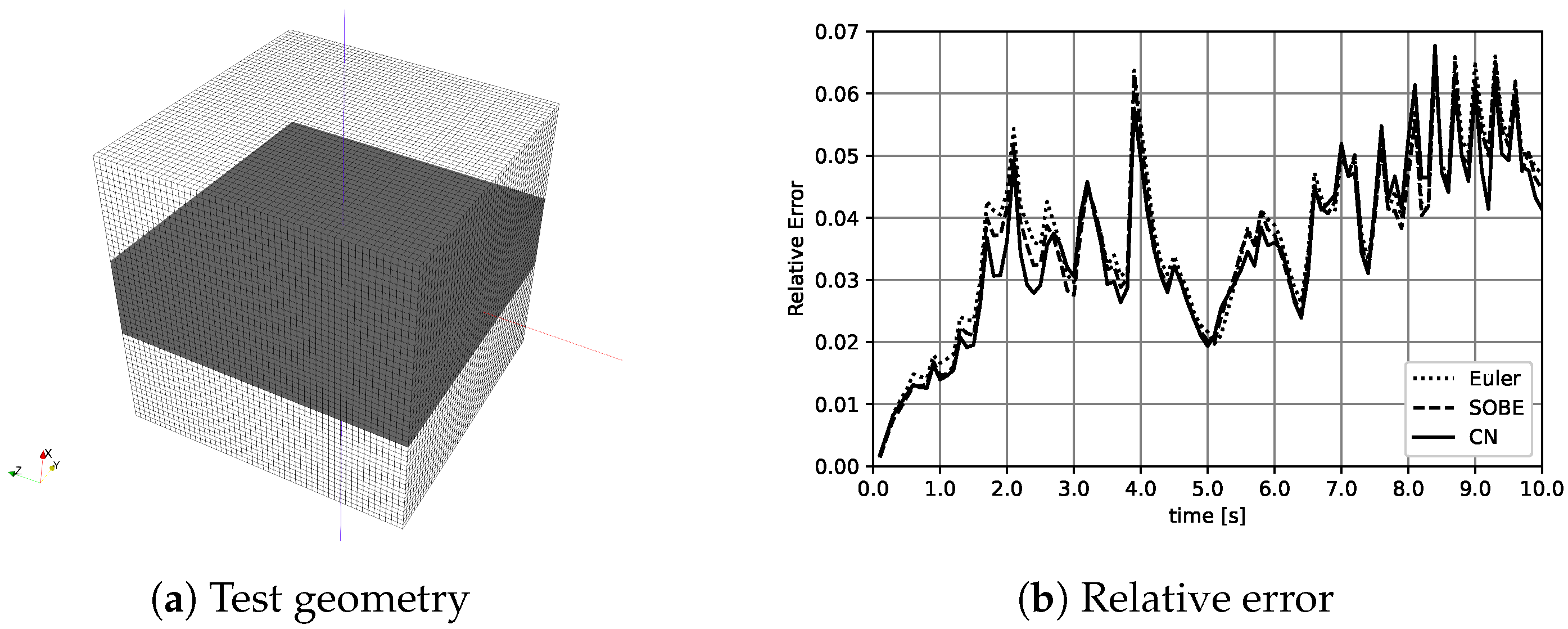
7. One-Dimensional Uniformly Accelerated Piston Test Case
7.1. Case Setup and Simulation Strategy
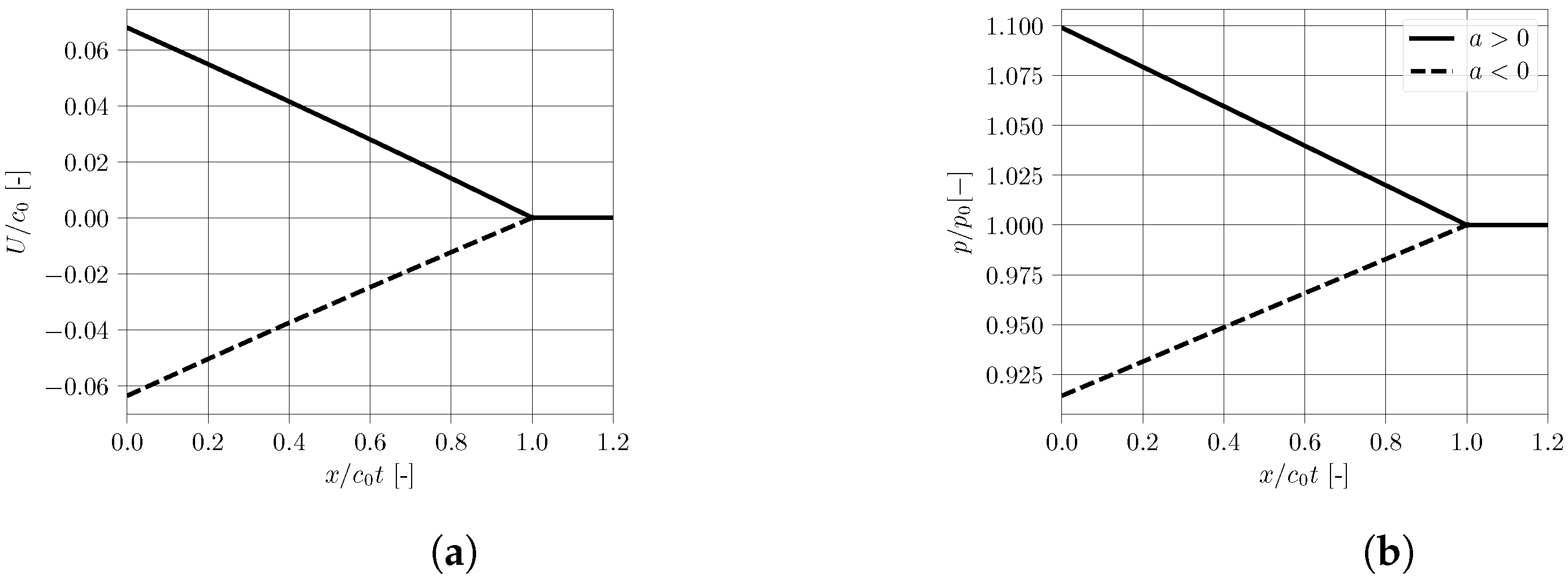
7.2. Code Verification
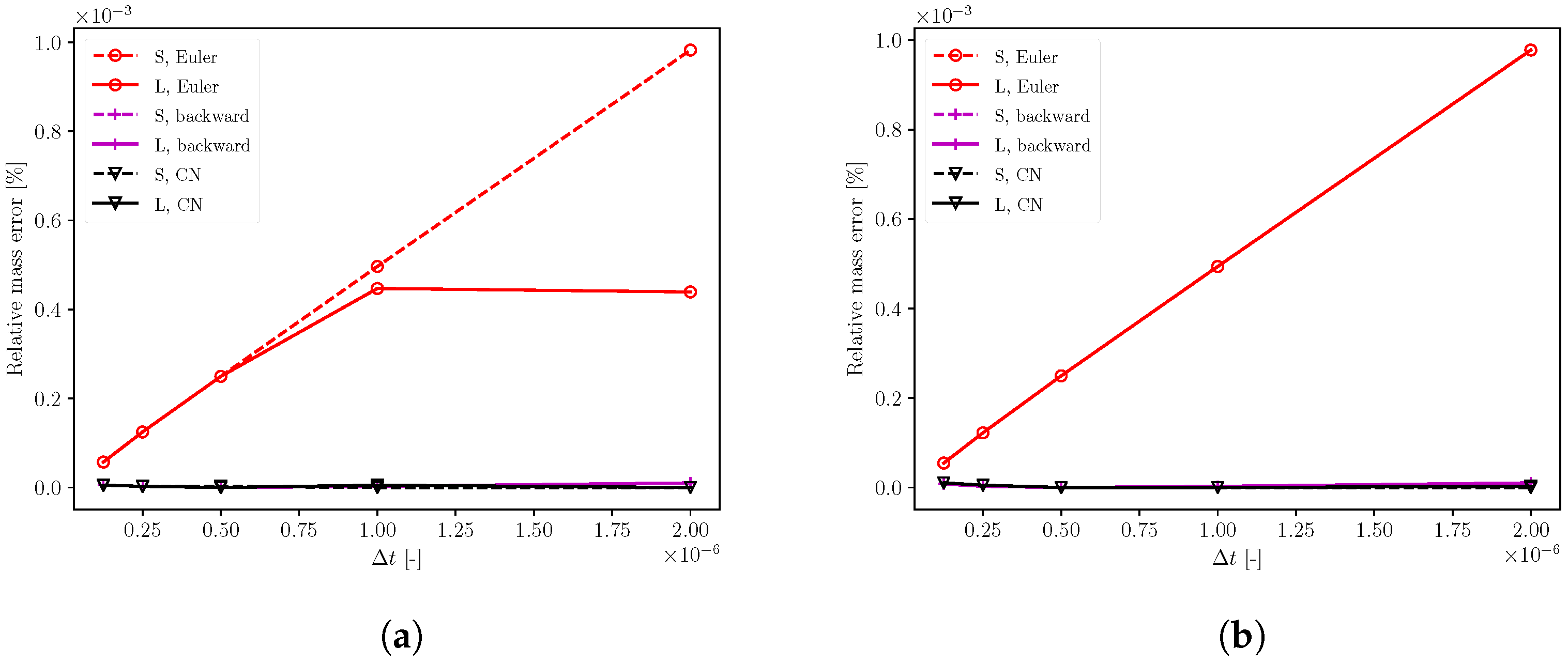
7.3. Mass Conservation
7.4. Temporal Order of Accuracy
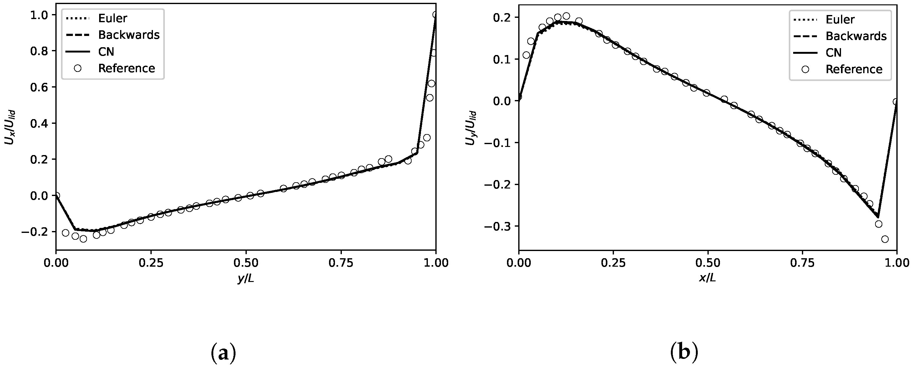
8. Lid-Driven Cavity Test Case
9. Conclusions
Author Contributions
Funding
Conflicts of Interest
Abbreviations
| ALE | Arbitrary Lagrangian Eulerian |
| DGCL | Discrete Geometry Conservation Law |
| SOBE | Second-Order Backward Euler |
| CN | Crank–Nicolson |
| AMR | Adaptive Mesh Refinement |
Appendix A. Crank–Nicolson Time-Differencing Scheme (CN)
References
- Baum, J.D.; Luo, H.; Löhner, R. A new ALE adaptive unstructured methodology for the simulation of moving bodies. In Proceedings of the Archives of Computational Methods in Engineering, Reno, NV, USA, 10–13 January 1994. [Google Scholar]
- Compère, G.; Remacle, J.F.; Jansson, J.; Hoffman, J. A mesh adaptation framework for dealing with large deforming meshes. Int. J. Numer. Methods Eng. 2010, 82, 843–867. [Google Scholar] [CrossRef]
- Hassan, O.; Sørensen, K.A.; Morgan, K.; Weatherill, N.P. A method for time accurate turbulent compressible fluid flow simulation with moving boundary components employing local remeshing. Int. J. Numer. Methods Fluids 2007, 53, 1243–1266. [Google Scholar] [CrossRef]
- Staten, M.L.; Owen, S.J.; Shontz, S.M.; Salinger, A.G.; Coffey, T.S. Proceedings of the 20th International Meshing Roundtable; Chapter A Comparison of Mesh Morphing Methods for 3D Shape Optimization; Springer: Berlin/Heidelberg, Germany, 2012; pp. 293–311. [Google Scholar] [CrossRef]
- Trulio, J.G.; Trigger, K.R. Numerical Solution of the One-Dimensional Hydrodynamic Equations in an Arbitrary Time-Dependent Coordinate System; Technical report; Report UCLR-6522; University of California Lawrence Radiation Laboratory: Berkeley, CA, USA, 1961. [Google Scholar]
- Trulio, J.G. Report No. AFWL- TR-66-19; Technical report; Air Force Weapons Laboratory: Kirtland Air Force Base, NM, USA, 1961. [Google Scholar]
- Hirt, C. An Arbitrary Lagrangian-Eulerian Computing Technique; Springer: Berlin/Heidelberg, Germany, 1971; Volume 8, Chapter 1; pp. 350–355. [Google Scholar] [CrossRef]
- Hirt, C.; Amsden, A.; Cook, J. An arbitrary Lagrangian-Eulerian computing method for all flow speeds. J. Comput. Phys. 1974, 14, 227–253. [Google Scholar] [CrossRef]
- Ferziger, J.; Perić, M.; Street, R.L. Computational Methods for Fluid Dynamics, 4th ed.; Springer: Berlin/Heidelberg, Germany, 2020. [Google Scholar] [CrossRef]
- Amsden, A.; O’Rourke, P.J.; Butler, T.D. KIVA-II: A Computer Program for Chemically Reactive Flows with Sprays; LA 11560-MS; Los Alamos National Laboratory: Los Alamos, NM, USA, 1989. [Google Scholar]
- Jasak, H.; Weller, H.G.; Nordin, N. In-cylinder CFD simulation using a C++ object-oriented toolkit. In Proceedings of the SAE Technical Paper 2004-01-0110; SAE International: Warrendale, PA, USA, 2004; p. 20. [Google Scholar] [CrossRef] [Green Version]
- Jasak, H.; Tukovic, Z. Automatic Mesh Motion for the Unstructured Finite Volume Method. Trans. FAMENA 2007, 30, 1–18. [Google Scholar]
- Montorfano, A.; Piscaglia, F.; Onorati, A. An Extension of the Dynamic Mesh Handling with Topological Changes for LES of ICE in OpenFOAM. In Proceedings of the SAE Technical Paper 2015-01-0384; SAE International: Warrendale, PA, USA, 2015; p. 20. [Google Scholar] [CrossRef]
- Demirdžić, I.; Perić, M. Space conservation law in finite volume calculations of fluid flow. Int. J. Numer. Methods Fluids 1988, 8, 1037–1050. [Google Scholar] [CrossRef]
- Demirdžić, I.; Perić, M. Finite volume method for prediction of fluid flow in arbitrarily shaped domains with moving boundaries. Int. J. Numer. Methods Fluids 1990, 10, 771–790. [Google Scholar] [CrossRef]
- Guillard, H.; Farhat, C. On the significance of the geometric conservation law for flow computations on moving meshes. Comput. Methods Appl. Mech. Eng. 2000, 190, 1467–1482. [Google Scholar] [CrossRef]
- Nobile, F. Numerical Approximation of Fluid-Structure Interaction Problems with Application to Haemodynamics. Ph.D. Thesis, Ecole Polytechnique Federale de Lausanne (EPFL), Lausanne, Switzerland, 2001. [Google Scholar]
- Farhat, C.; Geuzaine, P.; Grandmont, C. The Discrete Geometric Conservation Law and the Nonlinear Stability of ALE Schemes for the Solution of Flow Problems on Moving Grids. J. Comput. Phys. 2001, 174, 669–694. [Google Scholar] [CrossRef]
- Geuzaine, P.; Grandmont, C.; Farhat, C. Design and analysis of ALE schemes with provable second-order time-accuracy for inviscid and viscous flow simulations. J. Comput. Phys. 2003, 191, 206–227. [Google Scholar] [CrossRef]
- Farhat, C.; Geuzaine, P. Design and analysis of robust ALE time-integrators for the solution of unsteady flow problems on moving grids. Comput. Methods Appl. Mech. Eng. 2004, 193, 4073–4095. [Google Scholar] [CrossRef]
- Tukovic, Z.; Jasak, H. A moving mesh finite volume interface tracking method for surface tension dominated interfacial fluid flow. Comput. Fluids 2012, 55, 70–84. [Google Scholar] [CrossRef] [Green Version]
- Piscaglia, F.; Montorfano, A.; Onorati, A. Development of Fully-Automatic Parallel Algorithms for Mesh Handling in the OpenFOAM-2.2.x Technology; SAE Technical Paper 2013-24-0027; SAE International: Warrendale, PA, USA, 2013. [Google Scholar] [CrossRef]
- Piscaglia, F.; Montorfano, A.; Onorati, A. A Moving Mesh Strategy to Perform Adaptive Large Eddy Simulation of IC Engines in OpenFOAM. In Proceedings of the International Multidimensional Engine Modeling User’s Group Meeting 2014, the Detroit Downtown Courtyard by Marriott Hotel, Detroit, MI, USA, 7 April 2014; p. 20. Available online: https://piscaglia.aero.polimi.it/wp-content/uploads/2020/02/IMEM2014.pdf (accessed on 1 June 2023).
- Anderson, A.; Zheng, X.; Cristini, V. Adaptive unstructured volume remeshing–I: The method. J. Comput. Phys. 2005, 208, 616–625. [Google Scholar] [CrossRef]
- Loubère, R.; Maire, P.H.; Shashkov, M.; Breil, J.; Galera, S. ReALE: A reconnection-based arbitrary-Lagrangian–Eulerian method. J. Comput. Phys. 2010, 229, 4724–4761. [Google Scholar] [CrossRef] [Green Version]
- Loubère, R.; Maire, P.H.; Shashkov, M. ReALE: A Reconnection Arbitrary-Lagrangian–Eulerian method in cylindrical geometry. Comput. Fluids 2011, 46, 59–69. [Google Scholar] [CrossRef] [Green Version]
- Löhner, R. Three-dimensional fluid-structure interaction using a finite element solver and adaptive remeshing. Comput. Syst. Eng. 1990, 1, 257–272. [Google Scholar] [CrossRef]
- Alauzet, F. A changing-topology moving mesh technique for large displacements. Eng. Comput. 2014, 30, 175–200. [Google Scholar] [CrossRef]
- Wang, R.; Keast, P.; Muir, P. A comparison of adaptive software for 1D parabolic PDEs. J. Comput. Appl. Math. 2004, 169, 127–150. [Google Scholar] [CrossRef] [Green Version]
- Barlow, A.J. A compatible finite element multi-material ALE hydrodynamics algorithm. Int. J. Numer. Methods Fluids 2008, 56, 953–964. [Google Scholar] [CrossRef]
- Kucharik, M.; Shashkov, M.; Wendroff, B. An efficient linearity-and-bound-preserving remapping method. J. Comput. Phys. 2003, 188, 462–471. [Google Scholar] [CrossRef]
- Margolin, L.; Shashkov, M. Second-order sign-preserving conservative interpolation (remapping) on general grids. J. Comput. Phys. 2003, 184, 266–298. [Google Scholar] [CrossRef]
- Garimella, R.; Kucharik, M.; Shashkov, M. An efficient linearity and bound preserving conservative interpolation (remapping) on polyhedral meshes. Comput. Fluids 2007, 36, 224–237. [Google Scholar] [CrossRef]
- Re, B.; Dobrzynski, C.; Guardone, A. An interpolation-free ALE scheme for unsteady inviscid flows computations with large boundary displacements over three-dimensional adaptive grids. J. Comput. Phys. 2017, 340, 26–54. [Google Scholar] [CrossRef]
- Piscaglia, F. Developments in Transient Modeling, Moving Mesh, Turbulence and Multiphase Methodologies in OpenFOAM. In Proceedings of the Keynote Lecture at the 4th Annual OpenFOAM User Conference, Cologne, Germany., 11–13 October 2016. [Google Scholar]
- Landau, L.D.; Lifshitz, E.M. Physique Théorique–Tome VI Mécanique del Fluides; Éditions de Moscou: Moscow, Russia, 1971. [Google Scholar]
- The OpenFOAM® Foundation. Available online: http://www.openfoam.org/dev.php (accessed on 1 June 2023).
- Rhie, C.; Chow, W. A numerical study of the turbulent flow past an isolated airfoil with trailing edge separation. AIAA J. 1983, 21, 1525–1532. [Google Scholar] [CrossRef]
- Patankar, S. Numerical Heat Transfer and Fluid Flow; Hemisphere: New York, NY, USA, 1980. [Google Scholar]
- Peinado, J.; Ibáñez, J.; Arias, E.; Hernández, V. Adams–Bashforth and Adams–Moulton methods for solving differential Riccati equations. Comput. Math. Appl. 2010, 60, 3032–3045. [Google Scholar] [CrossRef] [Green Version]
- Hirsch, C. Numerical Computation of Internal and External Flows; Elsevier: Amsterdam, The Netherlands, 2007. [Google Scholar] [CrossRef]
- Martínez, J.; Piscaglia, F.; Montorfano, A.; Onorati, A.; Aithal, S. Influence of momentum interpolation methods on the accuracy and convergence of pressure–velocity coupling algorithms in OpenFOAM®. J. Comput. Appl. Math. 2017, 309, 654–673. [Google Scholar] [CrossRef]
- Crank, J.; Nicolson, P. A practical method for numerical evaluation of solutions of partial differential equations of the heat-conduction type. Math. Proc. Camb. Philos. Soc. 1947, 43, 50–67. [Google Scholar] [CrossRef]


 ,
,  and
and  ; for the Euler, SOBE and CN time schemes.
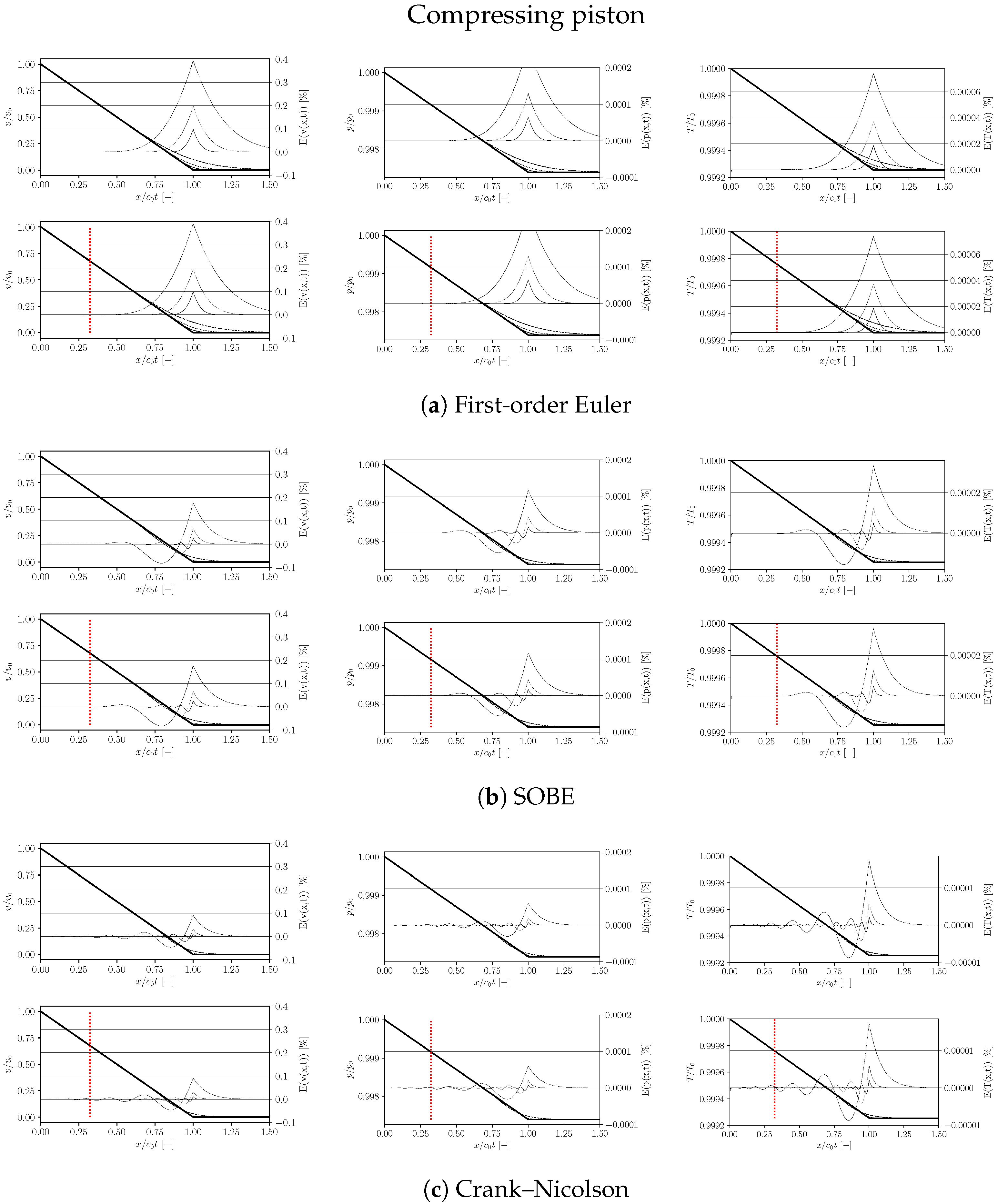
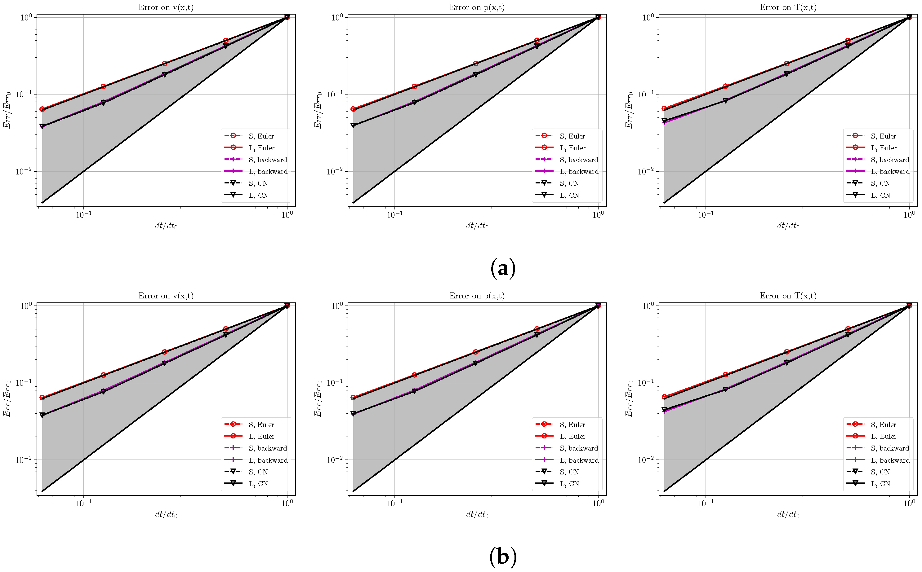
  represents the position of the dynamic layer. For each subfigure, from left to right, errors in velocity, pressure and temperature fields, respectively.
,
and ; for the Euler, SOBE and CN time schemes. represents the position of the dynamic layer. For each subfigure, from left to right, errors in velocity, pressure and temperature fields, respectively.
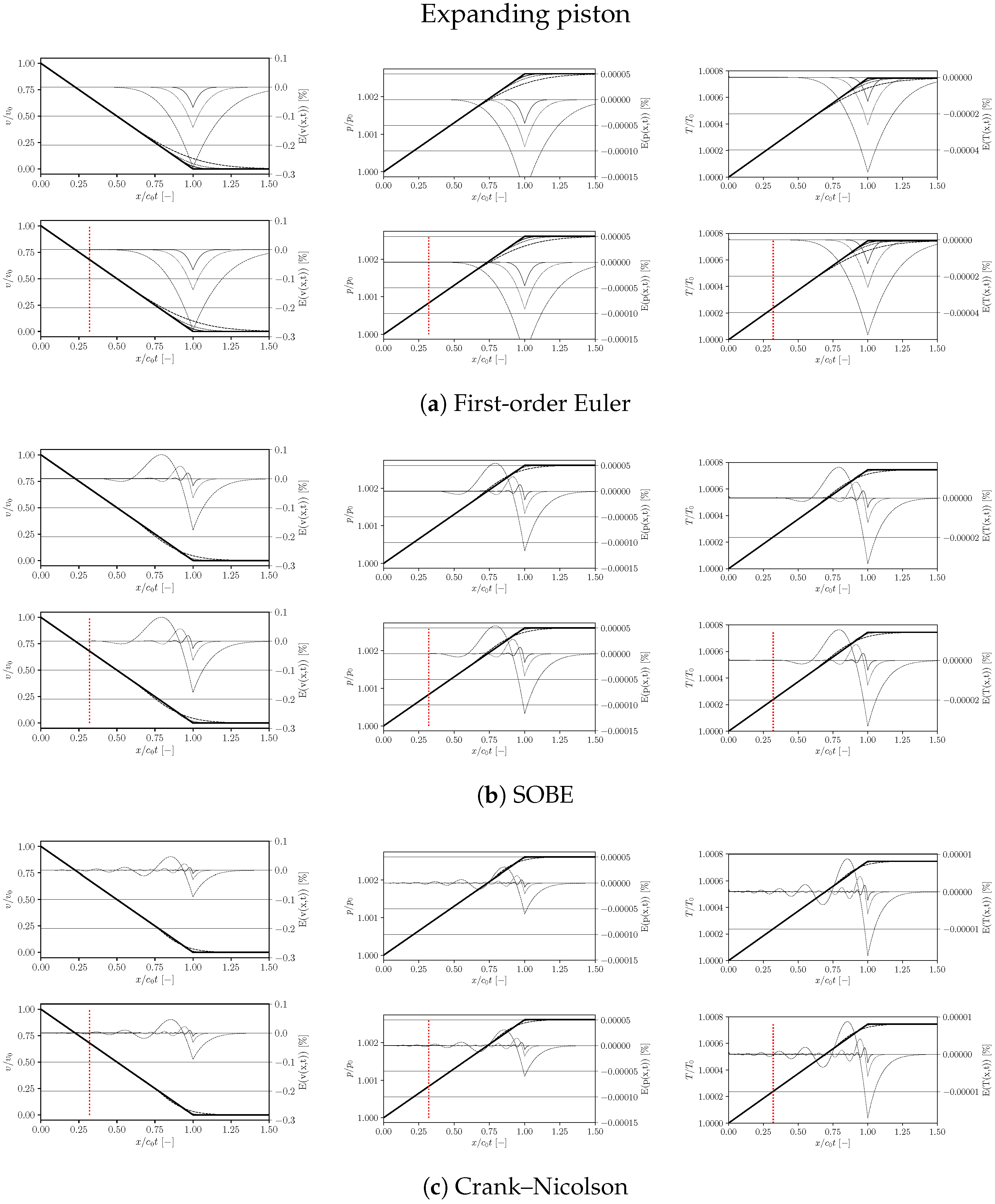
represents the position of the dynamic layer. For each subfigure, from left to right, errors in velocity, pressure and temperature fields, respectively.
,
and ; for the Euler, SOBE and CN time schemes. represents the position of the dynamic layer. For each subfigure, from left to right, errors in velocity, pressure and temperature fields, respectively. ,
and ; for the Euler, SOBE and CN time schemes. represents the position of the dynamic layer. For each subfigure, from left to right, errors in velocity, pressure and temperature fields, respectively.
,
and ; for the Euler, SOBE and CN time schemes. represents the position of the dynamic layer. For each subfigure, from left to right, errors in velocity, pressure and temperature fields, respectively.
,
and ; for the Euler, SOBE and CN time schemes. represents the position of the dynamic layer. For each subfigure, from left to right, errors in velocity, pressure and temperature fields, respectively.
,
and ; for the Euler, SOBE and CN time schemes. represents the position of the dynamic layer. For each subfigure, from left to right, errors in velocity, pressure and temperature fields, respectively.


| Variable | Values |
|---|---|
| Cell motion strategy | Cell stretching, layer A/R |
| Time scheme | Euler, SOBE, CN |
| 10,000 | |
| t (s) | 0.125, 0.25, 0.5, 1, 2 |
| Layer Removal | Layer Addition | |||||
|---|---|---|---|---|---|---|
| t | Euler | SOBE | CN | Euler | SOBE | CN |
Disclaimer/Publisher’s Note: The statements, opinions and data contained in all publications are solely those of the individual author(s) and contributor(s) and not of MDPI and/or the editor(s). MDPI and/or the editor(s) disclaim responsibility for any injury to people or property resulting from any ideas, methods, instructions or products referred to in the content. |
© 2023 by the authors. Licensee MDPI, Basel, Switzerland. This article is an open access article distributed under the terms and conditions of the Creative Commons Attribution (CC BY) license (https://creativecommons.org/licenses/by/4.0/).
Share and Cite
Costero, D.; Piscaglia, F. Second-Order Time-Accurate ALE Schemes for Flow Computations with Moving and Topologically Changing Grids. Fluids 2023, 8, 177. https://doi.org/10.3390/fluids8060177
Costero D, Piscaglia F. Second-Order Time-Accurate ALE Schemes for Flow Computations with Moving and Topologically Changing Grids. Fluids. 2023; 8(6):177. https://doi.org/10.3390/fluids8060177
Chicago/Turabian StyleCostero, Daniel, and Federico Piscaglia. 2023. "Second-Order Time-Accurate ALE Schemes for Flow Computations with Moving and Topologically Changing Grids" Fluids 8, no. 6: 177. https://doi.org/10.3390/fluids8060177