Article

The Perturbation of Ozone and Nitrogen Oxides Impacted by Blue Jet Considering the Molecular Diffusion

1
Key Laboratory of Middle Atmosphere and Global Environment Observation (LAGEO), Institute of Atmospheric Physics, Chinese Academy of Sciences, Beijing 100029, China
2
Department of Civil Engineering, Xi’an Jiaotong-Liverpool University, Suzhou 215123, China
*
Author to whom correspondence should be addressed.
Fluids 2023, 8(6), 176; https://doi.org/10.3390/fluids8060176
Submission received: 28 February 2023 / Revised: 31 May 2023 / Accepted: 6 June 2023 / Published: 7 June 2023

Abstract

:
This study investigated the diffusion impact on the chemical perturbation of NOx and O3 caused by the streamer and leader parts of a blue jet in the low stratosphere (18–30 km), using the coupling of a detailed stratospheric chemistry model and a typical diffusion model. The study found that diffusion significantly impacted the evolution of chemical perturbations at both short-term and long-term time scales after the blue jet discharge, with changes in NOx and O3 concentrations observed at different altitudes (18–28 km). At 18 km, the concentrations of NOx and N2O that account for diffusion start to decrease after 1 s, whereas those without diffusion remain at their peak concentrations. Meanwhile, O3 is slowly destroyed with less NOx, rather than dropping to an unrealistic low value immediately after the discharge without diffusion. The perturbation caused by the blue jet discharge disappears within a few tens of seconds at 18 km when molecular diffusion is considered. At 30 km, the chemical perturbation from four point sources was observed through changes in NO2 concentrations. However, the total concentration of NO2 perturbed by the streamer part discharge at the given surface was negligible when considering diffusion. Overall, this study provided a useful model tool for a more accurate assessment of the chemical effects of individual blue jets.

1. Introduction

The blue jet is an atmospheric discharge phenomenon that occurs in the stratosphere, propagating upward from the top of a thunderstorm to about 40–50 km [1,2,3,4]. It is classified as a transient luminous event (TLE). Similar to tropospheric lightning, blue jets also generate nitrogen oxides (NOx = NO + NO2) during their discharge processes and can perturb the ozone (O3) concentration of the atmosphere in which they occur [5]. Given that the altitude range of blue jets is located in the stratospheric ozone layer, the ionization process can produce nitrogen atoms (N), oxygen atoms (O), and NOx, which may disturb the chemical balance of the stratosphere; this was verified by Croizé et al. [6] based on a balloon experiment. Active nitrogen compounds can particularly affect the ozone layer through catalytic cycles. As the stratospheric ozone layer affects both the Earth’s climate and biosphere, it is crucial to accurately estimate the chemical impact of blue jets on stratospheric chemistry, particularly on the ozone layer. In recent years, ground-based and remote-sensing observations have found that blue jets are appearing more frequently, as reported by Chou et al. [7], and as a result, blue jets may have a significant impact on the stratospheric chemical system. Therefore, it is imperative to understand the chemical impact of blue jets on stratospheric chemistry and its effect on the ozone layer.
Previous studies on the chemical effects of blue jets have mainly utilized a box model approach, where the chemical effects of a blue jet discharge at a given point are studied without accounting for diffusion or any exchange of temperature or material quantity with the external environment. The focus has primarily been on the few seconds immediately following the discharge. Mishin [8] and Smirnova et al. [9] employed a simplified plasma chemical model, while Winkler et al. [10] developed a detailed plasma chemical model (including over 80 reactants and 1000 chemical reactions) to study the chemical effects of the blue jet streamers up to 100 s after discharge. Their simulation results revealed that ozone concentration increased by varying amounts after 100 s at 30 km, depending on the electric field values, chemical reaction types, and reaction rate coefficients used. Since the lifetime of ozone in the stratosphere is significantly longer than a few seconds, Xu et al. [11] conducted a study for the first time that focused on the chemical effects of blue jet streamers within two days after discharge based on a new plasm- chemistry model. Their findings showed an increase in ozone concentration during the first 100 s after the streamer discharge at 27 km. However, NOx, produced during the electric discharge process and has longer lifetimes of several hours or days, leads to ozone depletion through the catalytic cycle, resulting in even smaller ozone concentration than that without the discharge. These simulations indicated that the concentrations of NOx after the streamer discharge were almost 30 times higher than without discharge. Nonetheless, the effect of molecular diffusion was not considered in the two-day chemical effect simulation. As the concentrations of chemical species at each simulated time may significantly impact the result of chemical effect estimation, especially at a low altitude of the stratosphere, a significant error in the evaluation result could arise in stratospheric chemical simulations of hours or days if the diffusion effect is not taken into account. Therefore, there is a great need to incorporate the contribution of molecular diffusion in the chemical perturbation analysis.
Molecular diffusion is the thermal motion of gas particles due to their thermal energy at temperatures above absolute zero. This movement leads to a net flux of molecules from regions of higher concentration to those of lower concentration until a dynamic equilibrium is reached. The diffusion rate is affected by temperature, fluid viscosity, and particle size. Many studies have investigated the coupling effect of chemical processes and diffusion. Hami [12] developed a comprehensive model that considered the effects of convection, diffusion, and chemical reaction with several assumptions applied to the dispersion of pollutants in rivers at a steady state. Cheng et al. [13] developed a fully coupled diffusion-mechanic-reaction finite element method to simulate the oxidation of metallic materials at high temperatures. However, these studies mainly focused on diffusion and only considered linear functions for one pollutant reaction. To the best of our knowledge, this is the first attempt to consider the chemical reaction-diffusion coupling effect in the perturbation of NOx and O3 impacted by blue jet.
In this study, we evaluate the diffusion impact on the chemical perturbation caused by the streamer and leader parts of the blue jet at the low stratosphere (18–30 km) by coupling a stratospheric chemistry model with a diffusion model. Firstly, the chemical reaction-diffusion coupling model is set up with a diffusion time step, and the effect of other point sources on the studied point is assessed. The study then investigates the diffusion effects on the evolution of chemical reactions at short-term (the first 100 s) and long-term (48 h) time scales after the blue jet discharge from 18 to 28 km. Additionally, the study examines the diffusion effects on chemical perturbation with several point sources at 30 km by analyzing changes in NO2 concentrations. The finding of this study provides a research basis for an accurate assessment of the chemical effects of individual blue jets and their characterization on a regional or global scale.

2. Methods

2.1. Chemical Reactions Models

The chemistry model used in this study included 117 chemical species and 1760 chemical reactions. The time evolution of the concentration of each species is simulated through a thorough set of chemistry reactions in the stratosphere. Since we focused on nitrogen, oxygen species, and ozone perturbation, the main chemical reactions associated with O3, NO2, NO, and N2O are provided as an example. In this study, the chemical perturbation is simulated at night, so the relevant photochemical reactions are not considered. Equation (1) lists 5 of the whole (see the Supplementary Materials):
e + O 3 e + O 2 + O N + O 3 N O + O 2 O + O 3 O 2 + O 2 N O + O 3 N O 2 + O 2 N O 2 + O 3 N O 3 + O 2
The nonlinear system of chemical species evolution governing equations can be converted into a set of linear equations (a series of chemical ordinary differential equations (ODEs)) using a semi-implicit symmetric method by Ramaroson et al. [14]. It allows the conservation of the number of atoms and molecules. In this study, the first-order Forward Euler method (FE) is used to solve the chemical ODEs to estimate the chemical concentration change over time, in the form numerically:
d C ( t ) / dt = f ( C ( t ) , t )
where C is the molecular concentration (molec. cm−3), t is time (s), and f represents the total production and loss rates of chemical species in the reaction process that describes the derivatives of C with respect to t. The FE method is used to approximate the solution at discrete time steps, using the derivative of the solution at the current time step. The method starts with an initial value C (t0) at a given time t0, then repeatedly applies the derivative at each time step to estimate the solution at the next time step (t0 + t ). The method proceeds with chemical reactions by using the following formula:
C ( t 0 ) + t ) = C ( t 0 ) + t ( C P , t 0 C L , t 0 )
where t is the time step. C P = 1 m k m A m [ B m ] and C L = 1 n k n [ S ] A n are the chemical concentration of production and loss, respectively, where [ A ] and [ B ] are the concentration of reactants, [ S ] is the concentration of studied chemical species, k is the reaction rate, m and n are the numbers of reactions for the production and loss of chemical species. For instance, according to Equation (1), the total production and loss rates of species NO2 (Equation (2)), f( C N O 2 ( t ) , t ) = C P C L = k 4 × C N O ( t ) × C O 3 ( t ) k 5 × C N O 2 ( t ) × C O 3 ( t ) . ki is the chemical reaction rate in Equation (1).

2.2. Molecular Diffusion Models
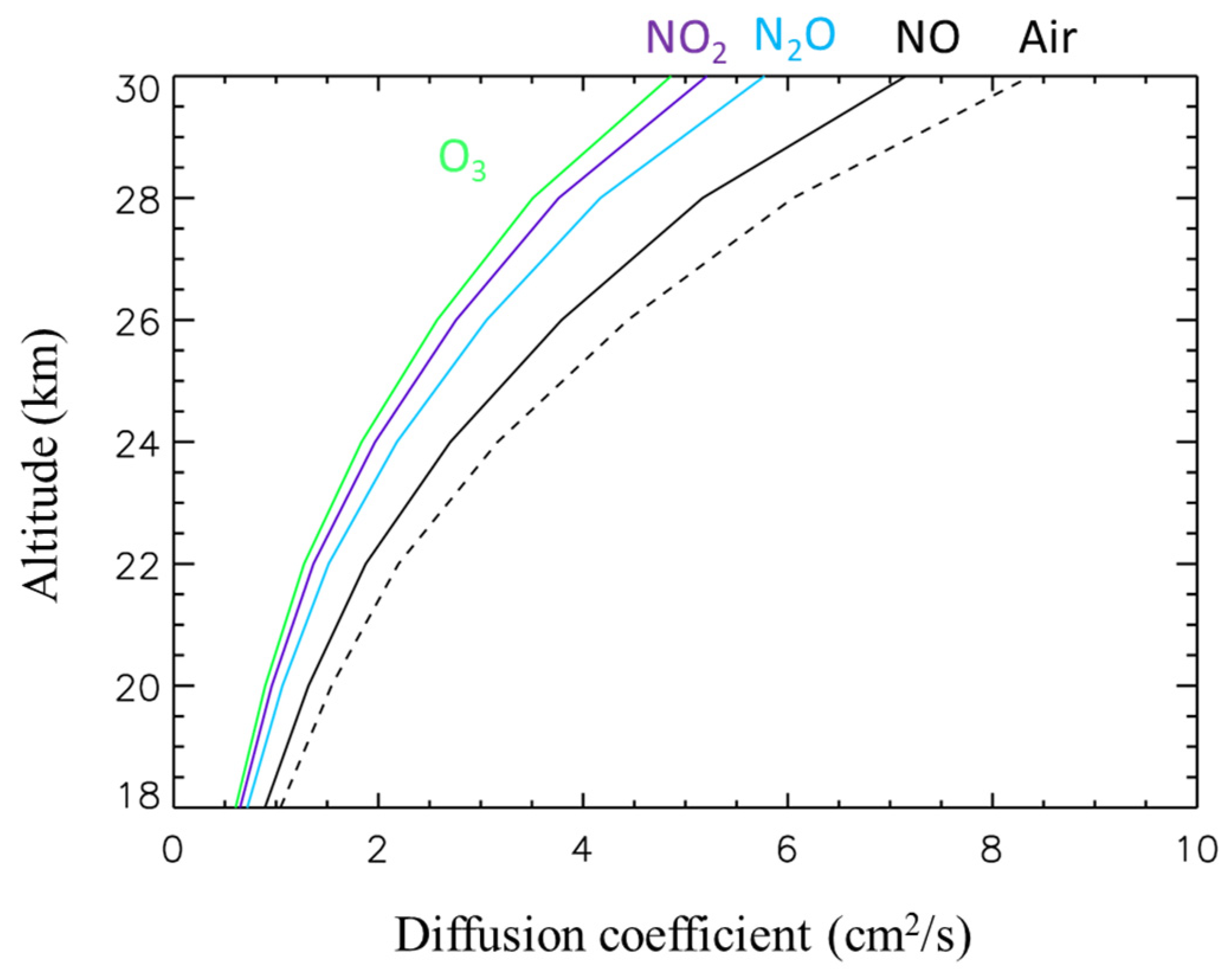
The streamer part of the discharge of the blue jet is assumed in this study to occur from 18 km to 50 km, and the leader part of the discharge occurs on average at 10−4 s, just after its streamer part discharge at one given point, which propagates from 18 km to 28 km, assumed in this study [15]. The peak concentration of the ozone layer distributes at the same altitude range as the leader part [16]. Moreover, the air concentration is greater at lower altitudes than at higher altitudes, resulting in a more significant impact of molecular diffusion at lower altitudes. As a result, this study focuses on investigating the coupling effect between chemical reactions and molecular diffusion at a given source point at altitudes ranging from 18 to 28 km (every 2 km), and at a given surface (30 km) with multisource points.
To consider the molecular diffusion in three dimensions, the study point of leader discharge is taken as an instantaneous source point in an environment with no mean wind. The diffusion equation is a parabolic partial differential equation (PDE):
C t = K x 2 C x 2 + K y 2 C y 2 + K z 2 C z 2
where K x , K y , and K z are the molecular diffusion coefficients or diffusivities in three directions, assumed to be constant and equal in a given direction in this study.
(a)
Diffusion coefficients of studied chemical species
Referred from Chapman and Cowling [17] and Davis [18], an expression for the diffusivity of trace gas chemicals in the air (cm2 s−1) with these characteristics is:
K x = 5 16 A d q 2 ρ a R * T m a 2 π ( m q + m a m q ) ,
where A is Avogadro’s number ( 6.0221367 × 10 23   m o l e c . m o l 1 ), dq is the collision diameter (cm) of gas chemicals molecule q, ρ a is air density (g cm−3), R * is the universal gas constant (8.31451 × 10 7 g cm2 s−2 mol−1 K−1), T is the absolute temperature (K), m a is the molecular weight of air (28.966 g mol−1), and m q is the molecular weight of gas chemicals q (g mol−1).
In our model, we assume the molecular diffusion coefficients at x, y, z directions are the same for the same species:
K x = K y = K z
Table 1 lists the collision diameters (CD, = 10 8 c m ), molecular weights (MW, g mol−1) of NO2, NO, O3, N2O, and their diffusion coefficients as a function of altitude from 18 km to 30 km. Among them, the collision diameters of NO2 and NO are taken from Halpern and Glendening [19]. Those of O3 and N2O are estimated by following the method of Halpern and Glendening [19], which used a simple computational approach from Wong et al. [20]. The diffusion coefficients of those chemical species at altitudes from 18 km to 30 km are obtained and shown in Figure 1. For the altitudes of interest (18–30 km), the diffusion coefficients of studied chemical species vary from 0.5 cm2 s−1 to 7 cm2 s−1.
  • (b) Analytical solution of the diffusion equation
The following boundary conditions are used for the stratospheric molecular concentration:
C x , y , z , t = = 0
C x 0 , y 0 , z 0 , t = 0 = 0 ,
0 C d x d y d z = Q i p ,
Based on these boundary conditions, the analytical solution of the diffusion Equation (4) is:
C = Q i p ( 4 π t ) 3 / 2 ( K x K y K z ) 1 / 2 × exp 1 4 t x 2 K x + y 2 K y + z 2 K z ,
where Q i p is the concentration at the source. The volume mixing ratios of NO2 and O3 are of the order of 10 ppb and 10 ppm (background value without the impacts of discharge, CBG) in the stratosphere during the night. Thus, in this study case (in the stratosphere and night-time), the boundary conditions (7) and (8), instead of C = 0 , the concentrations of NO2 and O3 are C N O 2 = 10   p p b × C ( a i r ) , C O 3 = 10   p p m × C ( a i r ) . Correspondingly, C in Equation (8) is the difference between the sources and the background concentration values. Considering the background air, the concentration of a particular chemical specie is:
C = Q i p ( 4 π t ) 3 / 2 ( K x K y K z ) 1 / 2 × exp 1 4 t x 2 K x + y 2 K y + z 2 K z + C B G ,
where C B G is the background concentration of the atmosphere.

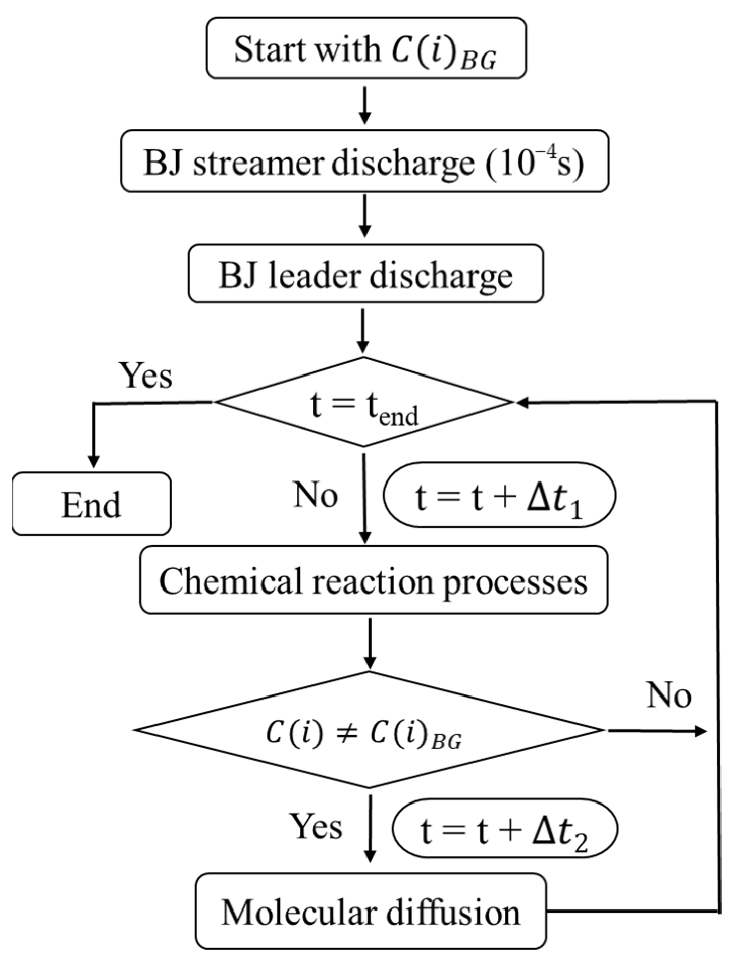
2.3. Coupling Chemical Reaction-Diffusion Processes

In order to consider the coupling effect of chemical reaction and diffusion, Equations (1) and (5) are combined to get the concentration at each time step. These chemical reaction-diffusion processes are described by parabolic PDEs for which the spatial coordinate is defined in the infinite domain [21]. The flowchart of the blue jet chemical effect considering the diffusion is shown in Figure 2. The time steps of the chemical reaction process ( t 1 ) and the diffusion process ( t 2 ) can be different. t 1 increases gradually from 10−6 s during the discharge process to 1 s, and t 2 will be evaluated in Section 3.1. The diffusion process occurs when the concentration of a chemical specie C ( i ) is different from its background concentration C ( i ) B G . The diffusion process ceases when the concentrations become equal and reach a dynamic equilibrium status. During the first time interval, gas chemistry and diffusion are solved sequentially.

3. Results and Discussions

3.1. Investigation of the Impact of Diffusion Parameters
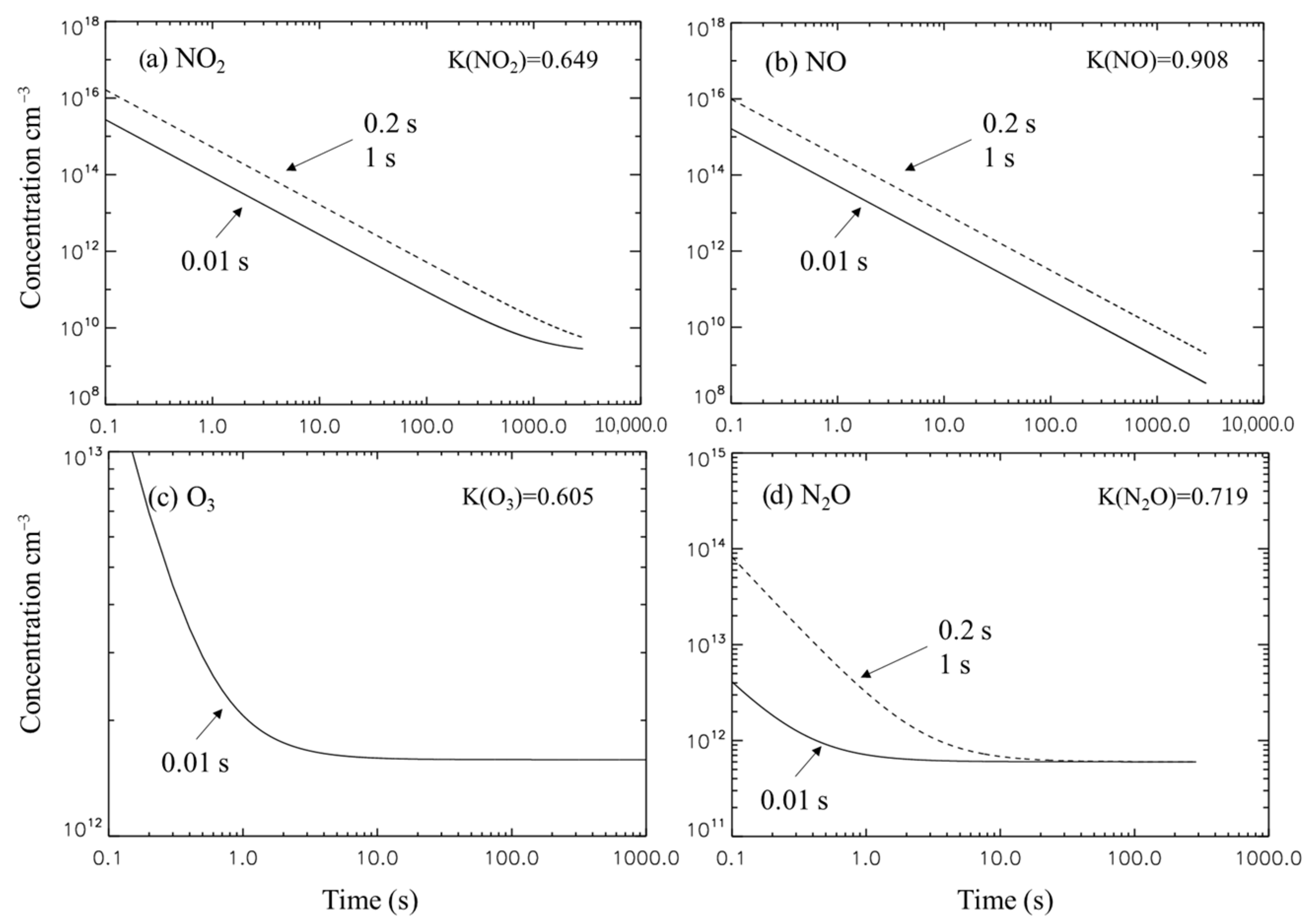
(a)
Estimation of time step in diffusion processes
To consider the diffusion of NO, NO2, O3, and N2O in this study, Table 1 displays the concentrations of NO2, NO, O3, and N2O after leader discharge in 10−2 s, 0.2 s, and 1 s at 18 km, for example. According to Table 2, the concentrations of NO2, NO, and N2O at the selected times exceed their background concentrations, and that of O3 only presents at 10−2 s. The concentration of chemical species at the source point (x = 0, y = 0, z = 0) affected by diffusion varies with time:
C = Q i p ( 4 π t ) 3 / 2 ( K x K y K z ) 1 / 2 + C B G
Therefore, the time evolutions of the chemical concentrations at selected times (10−2 s, 0.2 s, and 1 s) are shown in Figure 3. The time evolutions of NO2, NO, and N2O concentrations are the same for 0.2 s and 1 s diffusion and are represented by a single curve. However, the time step of 0.2 s and 1 s are too significant for O3 diffusion, resulting in a sharp decrease in concentration to its background value. Therefore, the related lines were not included in the figure. It is evident that all of their concentrations decrease rapidly over time. As a result, a diffusion time step ( t 2 ) of approximately 0.1 s, is adopted in this study.
  • (b) Evaluation of diffusion effect distance from other points of interest
Figure 4 shows the diffusion distributions of O3 at various distances from the points of interest in the x-y plane (z = 0). Assuming that the discharge source point (PA) is at x = 0, y = 0, even when the other point of interest (PB) is located at a distance of x = 50 cm, y = 50 cm from PA, it takes over 100 s for the diffusion of PB to impact PA. This time interval is longer than that used in the diffusion calculation process. Furthermore, the high-temperature core of the leader has a radius on the order of 103 cm [19], indicating that the diffusion of stratospheric background concentration can be neglected even for points on the edge of the leader core.

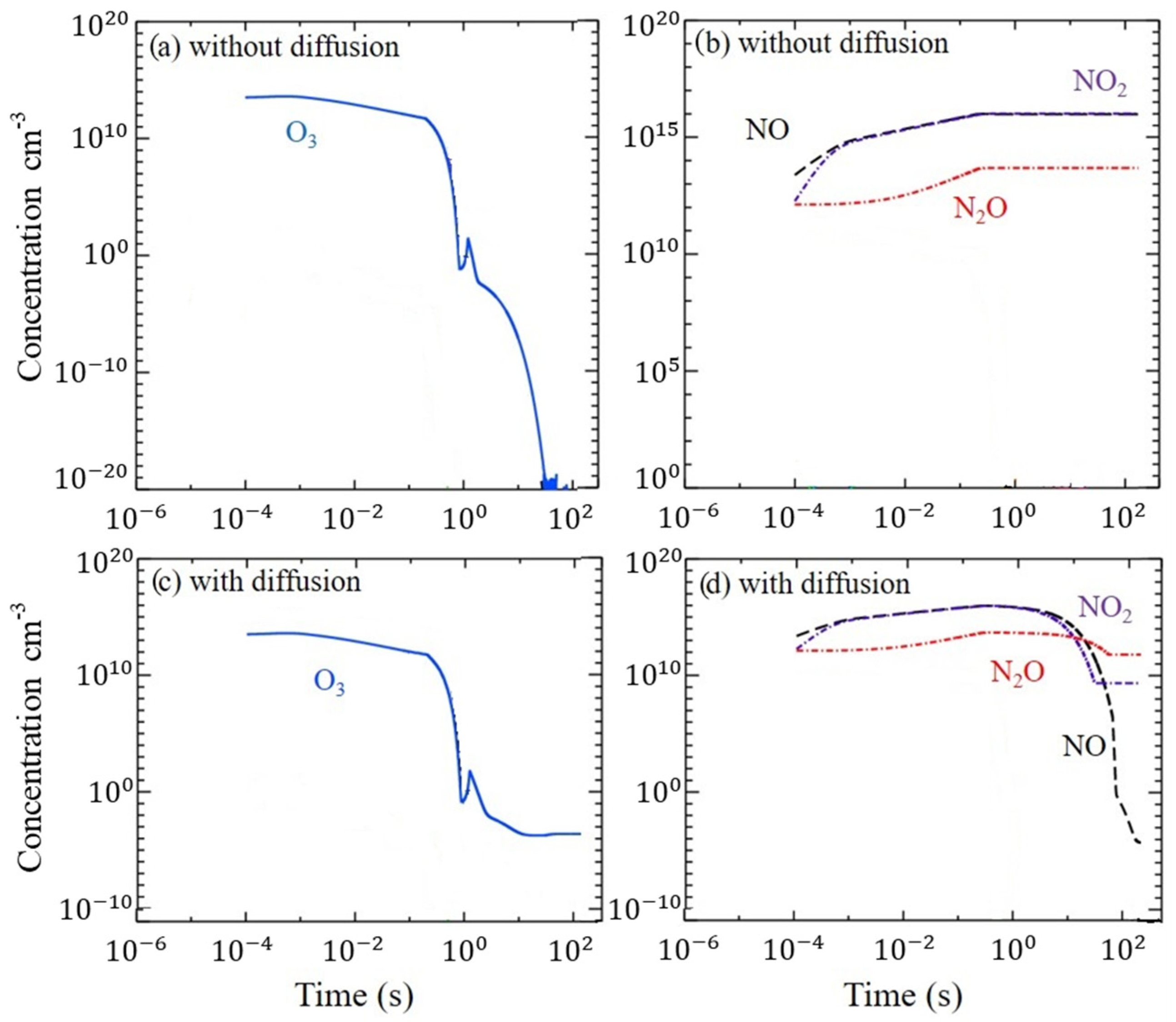
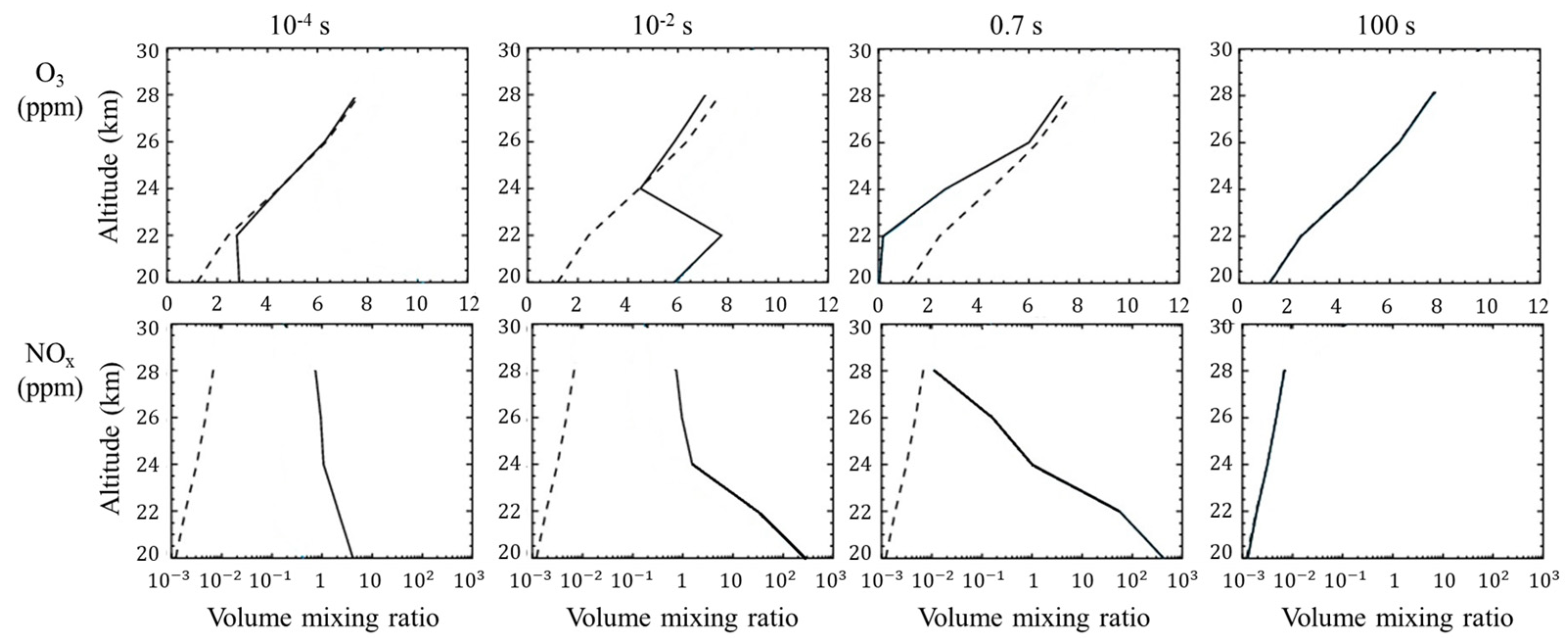
3.2. Diffusion Impacts in the Chemical Reaction Evolutions at 18–28 km

(a)
In the first 100 s after the blue jet discharge
The time evolutions of O3, NO2, NO, and N2O concentrations for the first 100 s after blue jet discharge are shown in Figure 5, at 18 km. Compared to Figure 20 and Figure 18 of Winkler et al. [10], the time variation of the chemical species studied, as shown in Figure 5c,d, exhibit similar sharp variations, which indicates that the model has been validated. The different concentrations observed in these two studies are attributed to variations in reaction rates and discharge process parameters utilized [11]. The diffusion has a notable impact on the evolution of these species during this period. Both NOx and N2O exhibit a similar increase initially, reaching their peak concentrations of 1016 cm−3 (Figure 5b,d). However, the concentrations of these species that account for diffusion start to decrease after 1 s, while those without diffusion remain at their peak concentrations. The diffusion impact decrease will stop until they reach their atmospheric concentrations. The time evolution of O3 shows that diffusion decreases to a meager value without considering diffusion, and the simulation oscillates (Figure 5a). The destroyed O3 is mainly due to the significant increase in NOx during the blue jet discharge through the catalytic cycle, which keeps the NOx concentration constant.
Nevertheless, when considering the diffusion of O3 and NOx in the chemical simulation, O3 is destroyed slowly with less NOx. Its constant night-time value is maintained (Figure 5c), significantly different from those without diffusion. The perturbation caused by the blue jet discharge disappears within a few tens of seconds at 18 km when molecular diffusion is considered.
Furthermore, compared to their background concentrations, the effects of blue jet discharge and diffusion differ at various altitudes. The volume mixing ratio (VMR) profiles of O3 and NOx between 20 to 28 km are shown in Figure 6 at specific times, of which the end of streamer and leader part discharge at 10−4 s and 10−2 s, respectively, and 0.7 s is the time when the high temperature caused by the leader part returns to natural temperature [10].
After the streamer discharge (10−4 s), O3 increased at low altitudes (below 24 km) while NOx increased from 10−3 ppm to 1 ppm at the studied altitudes. The rate of their increase is larger due to the higher concentration of O2 and N2 in the lower stratosphere. Following the blue jet discharge (10−2 s), NOx continued to increase, notably below 24 km. As a result of the increased NOx, O3 loss displays from 24 km to 28 km, with no notable increase in O3 impacted by the blue jet discharge. At 0.7 s, NOx decreases due to diffusion, although their VMRs remain more significant than the background VMR. Meanwhile, O3 VMR at all studied altitudes is destroyed to lower values than their background levels, with more significant decreases observed at lower altitudes. The impact of blue jet discharge at the studied altitudes disappears by the effect of diffusion, showing at 100 s.
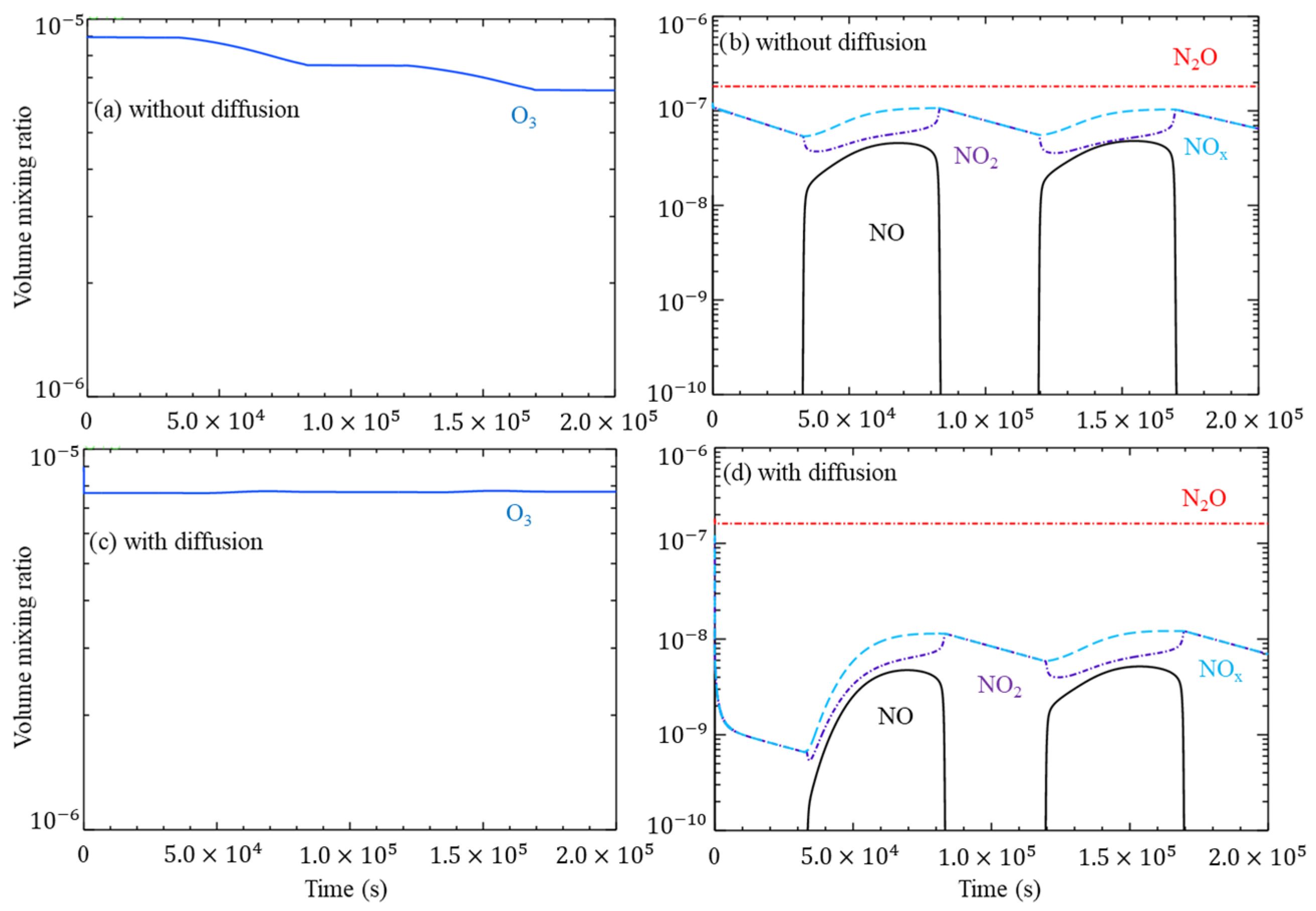
  • (b) In 48 h after blue jet discharge
After investigating the diffusion effects at a short-term scale, it is interesting to evaluate them at a long-term scale. In this part, we present the time evolutions of O3, NO2, NO, and N2O VMRs for the first 48 h after blue jet discharge, including both day and night cycles, at 28 km, as an example (Figure 7).
As demonstrated in the previous section, due to the diffusion effect, the VMRs of O3, NOx, and N2O after the blue jet discharge exhibit differences with and without diffusion. Without considering diffusion, the estimation of chemical impact by the blue jet discharge reveals that the produced NOx during the discharge processes maintains in two days (Figure 7b), and they destroy O3 VMR from 9 ×   10 6 to 6.4 ×   10 6 (Figure 7a). Conversely, with the diffusion, the NOx VMR decreases during the first day and maintains stable during the second day (Figure 7d), with its value being ten times smaller than that without diffusion Correspondingly, the time evolution of O3 remains constant at 7.6 ×   10 6 after two days (Figure 7c). Therefore, the diffusion effects are not only present at the short-term scale, mainly through molecular diffusion, but also at the long-term scale through chemical reaction processes due to the different concentrations of chemical species.

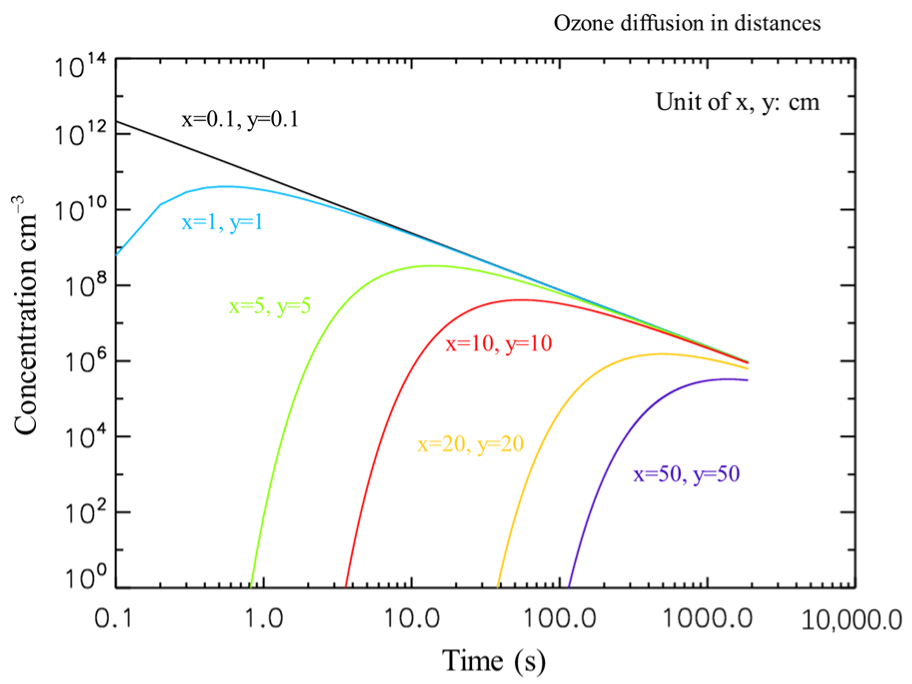
3.3. Diffusion Impacts of Multisource Points at 30 km

There are branches of streamers in the streamer zone of the blue jet. Therefore, the diffusion impact on chemical evolutions at the streamer zone is different from that at a given source point of streamer-and-leader occurrence at altitudes of 18–28 km (assumed in this study). The distance between individual streamers within the streamer zone would be:
d s = L s / N t o t a l 3
Here, L s is the observed streamer corona radius at the altitude, and N t o t a l is the total number of streamers at the height. Obviously, the d s varies significantly in the streamer zone, decreasing as the distance from the leader decreases. According to the physical properties of the blue jet described by Popov et al. [22], the average distance between streamers in the streamer zone is approximately 18.4 m.
To investigate the diffusion impacts on chemical evolutions at a given surface, this section presents the instantaneous distribution of four source points of NO2 concentrations at 30 km, with a distance of 18.4 m (Figure 8). The four source points are located in the x–y plane at (−9.2, −9.2) m, (−9.2, 9.2) m, (9.2, −9.2) m, and (9.2, 9.2) m, respectively, and have an initial concentration of 4.85 × 10 9 cm−3. Figure 8a–c evidently shows that the concentrations affected by diffusion at the source points decrease simultaneously from 4.85 × 10 9 cm−3 to 3.794 × 10 9 cm−3 between t = 0.25 s and t = 10 s, with a NO2 diffusion coefficient of 0.694 cm2/s. Eventually, the concentration drops to the background value of NO2 ( 3.79 × 10 9 cm−3) at t = 100 s (Figure 8d). Considering the diffusion at 30 km, the total concentration of NO2 perturbed by the streamer part discharge is very small on the given surface area of 1600 m2.

4. Conclusions

This study quantitatively investigated the coupling effects of chemical reaction-diffusion processes based on a detailed stratospheric chemistry model and typical diffusion model. The focus was on the perturbation of NOx and O3 in the streamer and leader parts of the blue jet in the low stratosphere. The chemical reaction-diffusion coupling model was initialized with an estimation diffusion time step of 0.1 s and with negligible effect from other points to the studied point sources.
The diffusion process had a notable impact on the evolution of chemical reactions at both short-term (the first 100 s) and long-term (48 h) time scales after the blue jet discharge from 18 to 28 km, resulting in the following: (1) the O3 concentration drops to an extremely low value immediately after the discharge without considering diffusion. However, the perturbation disappears within a few tens of seconds at 18 km. NOx and N2O initially increase to their peak concentrations of 1016 cm−3 and then decrease after 1 s due to diffusion, and the concentrations of studied chemical species are maintained constant. (2) The effects of blue jet discharge and diffusion vary at different altitudes. At altitudes below 24 km, O3 and NOx VMRs increase due to the larger amount of produced N and O concentration through the blue jet discharge processes at 10−4 s and 10−2 s. By contrast, NOx increases in smaller concentrations at 24 km to 28 km altitude. There is no significant increase in O3 VMRs, and they decrease to lower concentrations than those without discharge due to the O3 destroy catalytic cycle with NOx. At 0.7 s, NOx increases to a larger concentration below 24 km, and it decreases above 24 km. O3 is destroyed at all studied altitudes, with more destroyed concentration at lower altitudes. Due to the diffusion effect, the chemical perturbation disappears after 100 s. (3) At long-term scales (48 h) after the blue jet discharge, NOx VMR decreases on the first day due to diffusion and remains stable on the second day, with a VMR approximately ten times smaller than those without diffusion. O3 VMR remains at 7.6 ×   10 6 after two days, while it decreases from 9 ×   10 6 to 6.4 ×   10 6 without diffusion.
At an altitude of 30 km, where occurs branches of streamers, the chemical perturbation resulting from several point sources at a given surface is affected by diffusion, which are observed through changes in NO2 concentrations. In 1600 m2, with four source points at a distance of 18.4 m, the instantaneous distributions of NO2 concentrations at the point sources decrease simultaneously from 4.85 × 10 9 cm−3 to 3.794 × 10 9 cm−3 between diffusion durations of 0.25 s and 10 s. The NO2 concentrations eventually drop to their background values after 100 s of diffusion. Therefore, the total concentration of NO2 perturbed by the streamer part discharge is negligible at 30 km when considering diffusion.
This study first investigates the diffusion effect on the atmospheric discharge perturbed chemistry system, focusing on a limited number of main chemical species and the partial altitudes of blue jets. Further study could extend this investigation to include a more detailed analysis of chemical species and the whole range of altitudes where blue jets occur. Moreover, using a coupled chemical-diffusion model at each point source would be beneficial to obtain a more accurate estimation of the chemical-diffusion effect by blue jet at a given surface. Overall, this study provides a useful model tool as a research basis for a more accurate assessment of the chemical effects of an individual blue jet.

Supplementary Materials

The following supporting information can be downloaded at: https://www.mdpi.com/article/10.3390/fluids8060176/s1. Table S1: Main chemical reactions in blue jets. The rate coefficients are in units of s−1 for uni-molecular, cm3 s−1 for two-body reactions, and cm6 s−1 for three-body reactions. T is the gas temperature in Kelvin. M stands for N2 and O2 molecule. References [23,24,25,26,27,28,29] are cited in the Supplementary Materials.

Author Contributions

C.X., conceptualization; methodology; software; validation; formal analysis; investigation; writing—original draft preparation; supervision; funding acquisition; resources; data curation; W.Z., writing—review and editing; visualization; project administration; funding acquisition. All authors have read and agreed to the published version of the manuscript.

Funding

The research was supported by the National Natural Science Foundation of China (No. 42005093), the China Postdoctoral Science Foundation (No. E091021801), the RDF project (No. RDF-20-01-09), the Jiangsu Science and Technology Programme (No. RRSP10120220131), and the Jiangsu University Natural Science Research Programme (No. RRSP10120210150).

Data Availability Statement

Not applicable.

Acknowledgments

We would like to express our sincere gratitude to N. Huret, R. Fabrice, and S. Celestin for their invaluable contributions on the chemistry reaction model and their valuable advices to this study. We also thank the LPC2E (Le Laboratoire de Physique et de Chimie de l’Envi-ronnement et de l’Espace) for providing the computer server platform.

Conflicts of Interest

The authors declare no conflict of interest.

References

  1. Wescott, E.M.; Sentman, D.; Osborne, D.; Hampton, D.; Heavner, M. Preliminary results from the Sprites94 aircraft campaign: 2. Blue jets. Geophys. Res. Lett. 1995, 22, 1209–1212. [Google Scholar] [CrossRef]
  2. Wescott, E.M.; Sentman, D.D.; Stenbaek-Nielsen, H.C.; Huet, P.; Heavner, M.J.; Moudry, D.R. New evidence for the brightness and ionization of blue starters and blue jets. J. Geophys. Res. Space Phys. 2001, 106, 21549–21554. [Google Scholar] [CrossRef]
  3. Mishin, E.V.; Milikh, G.M. Blue jets: Upward lightning. Space Sci. Rev. 2008, 137, 473–488. [Google Scholar] [CrossRef]
  4. Pasko, V.P. Blue jets and gigantic jets: Transient luminous events between thunderstorm tops and the lower ionosphere. Plasma Phys. Control. Fusion 2008, 50, 124050. [Google Scholar] [CrossRef] [Green Version]
  5. Hiraki, Y.; Tong, L.; Fukunishi, H.; Nanbu, K.; Kasai, Y.; Ichimura, A. Generation of metastable oxygen atom O (1D) in sprite halos. Geophys. Res. Lett. 2004, 31, L14105. [Google Scholar] [CrossRef]
  6. Croizé, L.; Payan, S.; Bureau, J.; Duruisseau, F.; Thiéblemont, R.; Huret, N. Effect of blue jets on atmospheric composition: Feasibility of measurement from a stratospheric balloon. IEEE J. Sel. Top. Appl. Earth Obs. Remote Sens. 2015, 8, 3183–3192. [Google Scholar] [CrossRef]
  7. Chou, J.K.; Hsu, R.R.; Su, H.T.; Chen, A.B.C.; Kuo, C.L.; Huang, S.M.; Chang, S.C.; Peng, K.M.; Wu, Y.J. ISUAL-observed blue luminous events: The associated sferics. J. Geophys. Res. Space Phys. 2018, 123, 3063–3077. [Google Scholar] [CrossRef]
  8. Mishin, E.V. Ozone layer perturbation by a single blue jet. Geophys. Res. Lett. 1997, 24, 1919–1922. [Google Scholar] [CrossRef]
  9. Smirnova, N.V.; Lyakhov, A.N.; Kozlov, S.I. Lower stratosphere response to electric field pulse. Int. J. Geomagn. Aeron. 2003, 3, 281–287. [Google Scholar]
  10. Winkler, H.; Notholt, J. A model study of the plasma chemistry of stratospheric Blue Jets. J. Atmos. Sol.-Terr. Phys. 2015, 122, 75–85. [Google Scholar] [CrossRef]
  11. Xu, C.; Huret, N.; Garnung, M.; Celestin, S. A new detailed plasma-chemistry model for the potential impact of blue jet streamers on atmospheric chemistry. J. Geophys. Res. Atmos. 2020, 125. [Google Scholar] [CrossRef]
  12. Hami, M.L. A comprehensive model of functionals for three-dimensional non-isothermal steady flow with molecular and convective diffusion and a chemical reaction of arbitrary order. Chem. Eng. Sci. 2005, 60, 3693–3701. [Google Scholar] [CrossRef]
  13. Cheng, H.-J.; Zhang, X.-C.; Jia, Y.-F.; Yang, F.; Tu, S.-T. A finite element simulation on fully coupled diffusion, stress and chemical reaction. Mech. Mater. 2022, 166, 104–217. [Google Scholar] [CrossRef]
  14. Ramaroson, R.; Pirre, M.; Cariolle, D. A box model for on-line computations of diurnal variations in a 1-Dmodel-Potential for application in multidimensional cases. Ann. Geophys. 1992, 10, 416–428. [Google Scholar]
  15. Da Silva, C.L.; Pasko, V.P. Dynamics of streamer-to-leader transition at reduced air densities and its implications for propagation of lightning leaders and gigantic jets. J. Geophys. Res. Atmos. 2013, 118, 13–561. [Google Scholar] [CrossRef]
  16. Krueger, A.J.; Minzner, R.A. A mid-latitude ozone model for the 1976 US Standard Atmosphere. J. Geophys. Res. 1976, 81, 4477–4481. [Google Scholar] [CrossRef]
  17. Chapman, S.; Cowling, T.G. The Mathematical Theory of Nonuniform Gases; Cambridge University Press: Cambridge, UK, 1970. [Google Scholar]
  18. Davis, E.J. Transport phenomena with single aerosol particles. Aerosol Sci. Technol. 1983, 2, 121–144. [Google Scholar] [CrossRef]
  19. Halpern, A.M.; Eric, D. Glendening, estimating molecular collision diameters using computational methods. J. Mol. Struct. THEOCHEM 1996, 365, 9–12. [Google Scholar] [CrossRef]
  20. Wong, M.W.; Wiberg, K.B.; Frisch, M.J. Ab initio calculation of molar volumes: Comparison with experiment and use in solvation models. J. Comput. Chem. 1995, 16, 385–394. [Google Scholar] [CrossRef]
  21. Lefèvre, F.; Brasseur, G.P.; Folkins, I.; Smith, A.K.; Simon, P. Chemistry of the 1991–1992 stratospheric winter: Three-dimensional model simulations. J. Geophys. Res. Atmos. 1994, 99, 8183–8195. [Google Scholar] [CrossRef]
  22. Popov, N.A.; Shneider, M.N.; Milikh, G.M. Similarity analysis of the streamer zone of Blue jets. J. Atmos. Sol.-Terr. Phys. 2016, 147, 121–125. [Google Scholar] [CrossRef] [Green Version]
  23. Chipperfield, M.P. Multiannual simulations with a three-dimensional chemical transport model. J. Geophys. Res. Atmos. 1999, 104, 1781–1805. [Google Scholar] [CrossRef]
  24. Gordillo-Vázquez, F.J. Air plasma kinetics under the influence of sprites. J. Phys. D Appl. Phys. 2008, 41, 234016. [Google Scholar] [CrossRef] [Green Version]
  25. Kossyi, I.A.; Kostinsky, A.Y.; Matveyev, A.A.; Silakov, V.P. Kinetic scheme of the non-equilibrium discharge in nitrogen-oxygen mixtures. Plasma Sources Sci. Technol. 1992, 1, 207. [Google Scholar] [CrossRef]
  26. Sander, S.P.; Golden, D.M.; Kurylo, M.J.; Moortgat, G.K.; Wine, P.H.; Ravishankara, A.R.; Kolb, C.E.; Molina, M.J.; Finlayson-Pitts, B.J.; Orkin, V.L. Chemical Kinetics and Photochemical Data for Use in Atmospheric Studies Evaluation Number 15; Jet Propulsion Laboratory, National Aeronautics and Space Administration: Pasadena, CA, USA, 2006. [Google Scholar]
  27. Sentman, D.D.; Stenbaek-Nielsen, H.C.; McHarg, M.G.; Morrill, J.S. Correction to “Plasma chemistry of sprite streamers”. J. Geophys. Res. Atmos. 2008, 113, D14399. [Google Scholar] [CrossRef] [Green Version]
  28. Viggiano, A.A. Much improved upper limit for the rate constant for the reaction of O2+ with N2. J. Phys. Chem. A 2006, 110, 11599–11601. [Google Scholar] [CrossRef]
  29. Yaron, M.; Von Engel, A.; Vidaud, P.H. The collisional quenching of O2*(1Δg) by NO and CO2. Chem. Phys. Lett. 1976, 37, 159–161. [Google Scholar] [CrossRef]
Figure 1. Diffusion coefficients of studied chemical species (NO2, N2O, and NO) and air at 18 km to 30 km altitudes.
Fluids 08 00176 g001
Figure 2. Flowchart of the calculation of chemical diffusion-reaction coupling.
Fluids 08 00176 g002
Figure 3. The time evolutions of the concentrations of (a) NO2, (b) NO, (c) O3, and (d) N2O at selected times (10−2 s, 0.2 s, and 1 s) as the source point of diffusion at 18 km.
Fluids 08 00176 g003
Figure 4. Diffusion distributions of ozone at various distances from the points of interest in the xy plane.
Fluids 08 00176 g004
Figure 5. The time evolutions of the concentrations for O3, NO2, NO, and N2O both without diffusion (a,b) and with diffusion (c,d) during the first 100 s after the blue jet discharge at 18 km.
Fluids 08 00176 g005
Figure 6. The volume mixing ratio profiles of O3 and NOx at selected times (10−4 s, 10−2 s, 0.7 s, and 100 s) between 20 and 28 km. The dashed lines represent the values for the atmospheric background value without discharge impact, while the solid line represents the values impacted by the blue jet discharge and diffusion.
Fluids 08 00176 g006
Figure 7. The time evolutions of the VMRs for O3, NO2, NO, and N2O without diffusion (a,b) and with diffusion (c,d) during the first 48 h after the blue jet discharge at 28 km.
Fluids 08 00176 g007
Figure 8. The 3D view diffusion distributions of NO2 at different times: (a) t = 0.25 s (b) t = 1.0 s (c) t = 10 s, and (d) t = 100 s. The distributions are based on four source points located at a distance of 18.4 m in the streamer zone of 30 km.
Fluids 08 00176 g008
Table 1. The collision diameters (CD, 10 8 c m ), molecular weights (MW, g mol−1) of NO2, NO, O3, and N2O, and their diffusion coefficients (cm2/s) as a function of altitude from 18 km to 30 km.
Altitude (km)Temperature (K)NO2NOO3N2O
CDMWCDMWCDMWCDMW
4.422463.954304.56484.21944
18199.0160.6490.9080.6050.719
20207.140.6620.9270.6170.733
22211.130.6680.9360.6230.74
24218.5780.680.9520.6340.753
26222.6580.6860.9610.640.76
28224.3020.6890.9640.6420.763
30227.7940.6940.9720.6470.769
Table 2. The concentrations of NO2, NO, O3, and N2O after leader discharge (in 10−2 s, 0.2 s, 1 s) at 18 km, night-time.
GasAt 18 km, Night, T = 199.016 K
Diffusion
Coefficient (cm2/s)
Stratospheric
Concentration
(cm−3)
Concentration After Leader Discharge (cm−3)
10−2 s0.2 s1 s
NO20.649 2.28 × 10 9 2 × 10 15 1.2 × 10 16 1.2 × 10 16
NO0.9080 2 × 10 15 1.2 × 10 16 1.2 × 10 16
O30.605 1.58 × 10 12 1 × 10 13 9.0 × 10 11 0.2
N2O0.719 8.58 × 10 11 3 × 10 12 7.0 × 10 13 7 × 10 13
Disclaimer/Publisher’s Note: The statements, opinions and data contained in all publications are solely those of the individual author(s) and contributor(s) and not of MDPI and/or the editor(s). MDPI and/or the editor(s) disclaim responsibility for any injury to people or property resulting from any ideas, methods, instructions or products referred to in the content.

