Article

Suppression of the Spatial Hydrodynamic Instability in Scale-Resolving Simulations of Turbulent Flows Inside Lined Ducts

Laboratory of Computational Aeroacoustics and Turbulence, Peter the Great Saint-Petersburg Polytechnic University, 195251 Saint-Petersburg, Russia
*
Author to whom correspondence should be addressed.
Fluids 2023, 8(4), 134; https://doi.org/10.3390/fluids8040134
Submission received: 10 March 2023 / Revised: 8 April 2023 / Accepted: 12 April 2023 / Published: 17 April 2023
(This article belongs to the Special Issue Next-Generation Methods for Turbulent Flows)

Abstract

:
This paper addresses one of the major obstacles arising in the high-fidelity scale-resolving simulations of turbulent flows inside ducts with the walls covered by acoustic liners in order to attenuate the sound radiated from the duct. It consists of the development of spatial hydrodynamic (convective) instability over the treated walls at the low values of the acoustic resistance of the liner. For reasons that remain unclear, the growth rate of this instability and its effect on sound propagation through the duct is strongly overestimated by the CFD simulations using the macroscopic concept of the locally reacting acoustic impedance. A new damping volume source term (“body force”) is proposed, whose introduction into the momentum equation resolves this issue by means of artificially suppressing the instability while remaining within the framework of the computationally efficient model of the impedance wall, i.e., without trying to simulate the liner microscopically. Examples are presented of the application of the developed methodology to the flows in the grazing impedance tubes with two different liners. They suggest that the proposed form of the damping source term can be considered universal and that the suppression of the hydrodynamic instability ensured by this term is not accompanied by any significant distortion of the propagation of the sound waves and the turbulence statistics, except for a very narrow near-wall region.

1. Introduction

Acoustic wall treatment by installing lined panels is a major tool for reducing noise emission from the ducts of aircraft engines and ventilation/air-conditioning systems [1,2]. Therefore, an accurate prediction of the attenuation of sound waves enabled by the liners is of significant practical importance, and such a capability is very desirable for any computational fluid dynamics/computational aeroacoustics (CFD/CAA) numerical system aimed at the computation of the duct noise.
Unfortunately, for realistically complex problems, even the most powerful modern computers do not allow direct computation of turbulent flows over lined surfaces on the basis of the “microscopic” approach, i.e., with the resolution of the flow and sound wave propagation inside each liner cavity. For this reason, most of the computational studies in this area are performed with the use of some approximate approaches. Among them, the most widely spread one is the approach based on the macroscopic model of the locally reacting acoustic impedance, which was initially established for the linear acoustic computations in the Fourier (frequency) space. Specifically, assuming that the tangential velocity at the lined surface satisfies the no-slip boundary condition v τ = 0 , for a given angular frequency ω = 2 π f , the complex impedance of the liner Z ^ ( ω ) = R ( ω ) i X ( ω ) is defined by the following relation between the Fourier transforms (FT) of the acoustic pressure p ( t ) and the wall-normal velocity v n ( t ) = V ( t ) n at the wall [3]:
p ^ ( ω ) = Z ^ ( ω ) v ^ n ( ω ) ,
where the wall normal vector n is assumed to point inside the liner, R and X are the acoustic resistance and reactance, respectively, i ( 1 ) 1 / 2 , and the time-dependence of the harmonic signal is assumed to have the form exp ( i ω t ) .
This relation is the impedance boundary condition (IBC), which replaces the standard non-permeability condition v n = 0 imposed at the solid wall. Note that if the flow over a liner is described in the framework of the inviscid gas dynamic models (e.g., the linearized Euler equations), which assume non-zero tangential velocity at the wall, the simplest IBC (1) should be replaced by a more complicated Ingard–Myers condition [4]. However, such models and boundary conditions are beyond the scope of the present paper.
In order to make this approach compatible with more general non-linear flow models and the CFD solvers in use, the IBC must be translated from the Fourier space into the time domain. Although ensuring the well-posedness of the corresponding problem statement is far from trivial (see, e.g., Rienstra [5]), extensive research in this field, starting with the pioneering work of Tam and Auriault [6], resulted in a number of time-domain impedance models (TDIMs) (see, e.g., [7,8,9,10,11,12,13]), which can be used in practical computations of sound propagation in lined ducts in the framework of aerodynamic flow models of different complexity. In particular, the author’s earlier work [13] presents an advanced version of the TDIM [11,12] (the “Auxiliary Differential Equation” or ADE model), which is specially adapted for application in combination with scale-resolving approaches to turbulence representation. Note that such approaches, allowing a direct resolution of the processes of noise generation due to the interaction of vortical turbulent structures with each other and with solid surfaces, are the core of modern numerical non-empirical aeroacoustic systems.
However, at low values of the acoustic resistance of the liner, scale-resolving simulations of the flow/acoustics inside the lined ducts with the use of the IBC face serious difficulties. It consists of spatial hydrodynamic (convective) instability, which can develop in a narrow layer adjacent to the impedance wall and contaminate the acoustic predictions because the simulations incorrectly reproduce the instability characteristics.
A fairly illustrative example can be found in the aforementioned work [13], in which the instability is observed in the simulations reproducing benchmark experiments [14] on the sound propagation in turbulent flow inside NASA’s grazing incidence tube (GIT) with the use of wall-modeled large eddy simulations (WMLES) based on the IDDES hybrid RANS-LES model [15]. It is expressed most strongly when the frequency of the external waves injected into the duct (the frequency of the forcing signal fe) is equal to 1000 Hz, which value is close to the resonant frequency fRES = 1040 Hz of the tested ceramic tubular liner CT57 (at this frequency, the liner’s normalized acoustic resistance, R / ( ρ c ) , reaches the minimum of ~0.4), and manifests itself in the formation of periodic large-scale structures in the close vicinity of the lined wall. These structures have a rather large correlation length in the spanwise direction (they are nearly 2D) and are convecting along the wall at a velocity of about 70% of the bulk flow velocity, with the amplitude of the instability wave growing while moving downstream. This causes a substantial alteration of both the turbulence characteristics (intensity of the fluctuations and their spectra) and the parameters of the mean flow in the near-wall area. Judging by the experimental distributions of the sound pressure level (SPL) along the duct wall [14], in the real GIT flow, a minor instability must be present as well. However, the WMLES [13] drastically overemphasizes its growth rate, which results in quite poor agreement with the experiment. Moreover, in the simulations, the instability waves at the resonant frequency are observed not only in the case of the near-resonant external forcing but also at all the other tested forcing frequencies and even in the case when there is no forcing signal. These prominent features of the hydrodynamic instability found in [13] are illustrated by sample results from the simulations [13] in Figure 1, Figure 2 and Figure 3 included in the present paper for the sake of self-containment. The instability originates from a very narrow area adjacent to the lined wall and supposedly has an inviscid nature resembling the Kelvin-Helmholtz instability [16,17]. It should be emphasized that the instability observed in the WMLES solutions [13] has a physical rather than numerical origin, and its characteristics are not affected significantly by a strong grid-refinement.
In this context, it should be noted that the occurrence of the spatial hydrodynamic instability in the flows along lined surfaces was observed in a number of both experimental and theoretical/numerical studies (a representative list can be found in [16,17,18,19,20,21,22,23]). However, as of today, the interpretation of this phenomenon in the literature remains rather contradictory.
On the experimental side, it is firmly established that the instability is real and is observed for the liners with low normalized acoustic resistance ( R / ( ρ c ) less than ~0.5) at the frequencies of the external sound waves close to the resonant frequency of the liner. This is directly demonstrated, e.g., by the optical measurements of Marx et al. [19]. At the same time, according to Rienstra and Vilenski [16] and Rienstra and Darau [21], in practical problems, the instability is very weak or not present at all and, particularly, has never been detected in the ducts of turbofan engines, which represent the main area of application of acoustic liners.
In the theoretical/numerical studies, the instability is revealed by the linear stability analysis (LSA) based on both the linearized Euler and the linearized Navier–Stokes equations (see, e.g., [17,24,25,26]) and is observed in many computational works [13,16,20,27,28,29], in which it displays in very different forms. Specifically, the growth rate of the instability depends on the specific flow model, the formulation and details of the implementation of IBCs, and the numerics used. In most cases, similar to what is observed in [13], it is significantly overestimated. In the present author’s opinion, this is probably a reflection of the fact that an adequate representation of the spatial hydrodynamic instability in the flows over lined walls on the basis of the macroscopic concept of the acoustic impedance is just impossible and that any model that claims to be reliable in predicting the instability characteristics should be based on the microscopic approach, that is, should include a detailed description of the hydrodynamics and acoustics inside each cavity of the liner. However, as already mentioned, as applied to practical problems, this approach requires very large (currently unaffordable) computational resources.
In this situation, the “pragmatic” computational strategy seems to be to give up the claim of accurately reproducing the instability and artificially suppress it instead. If successful, this would result in a much weaker deterioration of the solution than that caused by the drastic overestimation of the growth rate of the instability in the simulations.
This strategy has been adopted recently in the work of Deng et al. [17] in the framework of the linearized Euler equations (LEE) used in their study for the solution of the same problem as that considered in [13] and outlined above, i.e., for computing the propagation of the plane sound waves in the NASA GIT with ceramic tubular liner CT57 [14]. This approach, called by the authors of [17] “partial gradient term suppression” (PGTS), presents a special version of a more general method (“gradient term suppression (GTS)) by Bogey et al. [30], proposed for stabilization of the acoustic computations based on the LEE and, particularly, the jet-noise prediction. In essence, it reduces to introducing an artificial damping volume source term (“body force”) into the original governing equations. It is shown in [17] that this stabilization method really allows for suppressing the unstable hydrodynamic modes of the time-domain LEE solution but has a serious side effect of a noticeable alteration of the acoustic modes, especially at low Helmholtz numbers f L / c . More important in the context of the present study is that, as shown in Section 3 below, combining this method with the scale-resolving simulations of turbulent flows over lined surfaces results in a significant distortion of the intensity of turbulent fluctuations, whose correct representation is the basic requirement for the application of the scale-resolving approaches to aeroacoustic problems.
Exactly this was the motivation for an attempt undertaken in the present work to devise a new numerical tool capable of eliminating the hydrodynamic instability with no or, at least, a much less harmful effect on the prediction of the turbulence statistics and, in addition, being more accurate in terms of acoustics. An outcome of this work is presented in the remainder of the paper, which is organized as follows:
In Section 2, we present a brief description of the flows and experimental data used for tuning and testing the developed approach, together with some numerical details. Then, in Section 3, a step-by-step design is outlined for a new artificial volume source term (stabilization body force) that is compatible with the turbulence-resolving simulations, and satisfies the demands formulated above. The efficiency of the approach is then compared with the method of Deng et al. [17] in terms of the deterioration of the acoustic modes and the level of distortion of the predictions of the turbulent pulsations. In addition, the sensitivity of the predictions to the body force parameters is analyzed. Finally, in Section 4, the universality of the developed approach is demonstrated by means of its application to an alternative single-degree-of-freedom (SDoF) acoustic liner with a perforated facesheet representative of the liners widely used for the reduction of the turbofan engines noise. In Section 5, some conclusions are formulated.
Partly, the results of this work were presented earlier in the conference paper [31].

2. Flows under Consideration and Some Numerical Details

2.1. Ducts Geometries and Flow Regimes

In this work, we compute the flowfields in the two different impedance tubes with the grazing turbulent flow, which were used in the NASA experiments [14,32] devoted to the investigation of the effect of the acoustic liners on the sound wave propagation inside ducts. Schematics of these flows are shown in Figure 4a,b, respectively.
The first of them is the already mentioned flow in the NASA Grazing Incidence Tube (GIT) with the ceramic tubular acoustic liner CT57, which has a resonant frequency close to 1000 Hz. The corresponding experimental data [14] are currently considered a standard benchmark for the evaluation of the capabilities of the numerical/modeling approaches to the prediction of sound propagation in ducts with acoustically treated walls (see, e.g., [7,9,10,29,33]). In the present work, the GIT flow serves as the main testbed for the design of the stabilization body force and its tuning.
The GIT test section is the square duct with a width and height of Ly = Lz = H = 0.0508 m and a length of Lx = 0.8228 m. The liner sample covers a part of the upper wall of the test section, starting at x = 0.02032 m and ending at x = 0.6096 m. The plane sound waves in the experiment are introduced at the inlet of the test section (at x = 0), and their intensity is automatically adjusted to ensure that the SPL at the center of the lower wall at x = 0 is equal to 130 dB. The acoustic pressure is measured along the centerline of the lower wall of the test section. The measurements are performed at six different frequencies of the external acoustic forcing fe within the range (500–3000) Hz with a 500 Hz increment.
The current computations are performed for the flow regime with the area-averaged Mach number MAV = 0.335 in the reference measurement cross-section (x = 0.356 m), for which the measured Mach number field is available in [14]. It should be noted that the published NASA GIT experimental papers [14,34] do not provide the duct geometry upstream of the test section, which makes accurate reproduction of the experimental velocity profiles in the simulations problematic. An investigation and discussion of the sensitivity of the predictions to the shape of the inflow velocity profile can be found in [13].
The second flow considered in the present work (see Figure 4b) is that in the NASA grazing flow impedance tube (GFIT), which was used in the recent experiments [32] for the investigation of the properties of a set of the SDoF acoustic liners with perforated facesheet. Their typical feature is a significant dependence of the acoustic impedance on the sound wave intensity (the level of the root-mean-square pressure pulsations, p R M S ). This is different from the ceramic tubular liner tested in [14], and if the p R M S distribution along the lined wall is not known a priori, it strongly complicates the simulations in the framework of the linear impedance models. However, the “dynamic impedance” approach proposed in [13] and used in the present work allows an efficient overcoming of this difficulty. Earlier, in the conference paper [31], we performed the simulations of the sound propagation inside NASA GFIT with the use of the unsteady Reynolds-averaged Navier-Stokes equations (URANS) for the four liners [32] having different acoustic properties, particularly the acoustic resistance. In the present work, the scale-resolving WMLES simulations are carried out for one of these liners, specifically, the liner AE02 [32], which has the lowest resistance and, therefore, the strongest trend toward forming the instability wave in the flow over the lined wall.
The test-section of the GFIT [32] presents a rectangular (rather than square) duct of length Lx = 1.27 m with the cross-section dimensions Ly × Lz = 0.0635 m × 0.0508 m. The liner sample is placed on the upper wall at 0.284 m ≤ x ≤ 0.69 m. Similar to the GIT experiment, the SPL of the waves propagating inside the GFIT test section is measured along the centerline of the lower duct wall opposite the liner. In addition, some measurements are performed on its upper wall outside of the lined part of the surface. The measurements in [32] are carried out for the external acoustic forcing (injection of the plane sound waves) at a number of frequencies within the range (400–3000) Hz. The intensity of the injected waves at x = 0 (at the location of the first microphone) is equal to 140 dB.
The hydrodynamic measurement section in the GFIT is located at x = −0.143 m, i.e., slightly upstream of the acoustic test section. In contrast to the GIT [14], before entering the test section, the GFIT flow passes through a long (about 4 m) straight duct, which facilitates reproducing in the simulations the experimental flowfield (the Mach number) within the test section. The computations are performed for the flow regime identified in the experiments [32] as the regime with the Mach number M = 0.5 (this is the Mach value at the centerline “at some cross-section close to the duct exit”). According to [32], in this regime, the Mach number averaged over the measurement cross-section is MAV = 0.362, and within the test section, it gradually increases up to the value of ~0.4 at x, corresponding to the middle of the liner.

2.2. Computational Problem Statement

The computations of the flows and the plane sound wave propagation in the two experimental facilities described above are carried out with the use of the WMLES approach based on the IDDES method [15]. The computational model functions in the zonal RANS-WMLES framework. This includes using the volumetric synthetic turbulence generator (VSTG) [35] located in the vicinity of the RANS-WMLES interface in order to trigger the WMLES mode of the IDDES. It should be emphasized that the VSTG [35] ensures the rapid transition from the RANS to the WMLES with virtually no damage to acoustics, i.e., without generation of any noticeable spurious noise (see [13]), as is typical of most of the existing approaches to “creation” of a turbulent content at the (WM)LES inflow.
The computations are based on a two-stage procedure.
In its first stage, precursor steady-state RANS computations are performed for the flows in the solid-wall ducts (with no acoustic wall treatment) and without any external acoustic signal. These computations are carried out in long computational domains and ensure matching the experimental values of the section-averaged Mach number profiles in the measurement cross-sections of the modeled facilities (MAV = 0.335 at x = 0.356 m for the GIT [14] and MAV = 0.362 at x = −0.143 m for the GFIT [32], see Figure 4).
The precursor computations serve mainly to define the inflow velocity profiles for imposing the boundary conditions for the second (“production”) stage, in which the propagation of sound waves in the ducts with the liners installed on their upper walls is computed with the use of the zonal unsteady RANS (URANS)-IDDES model combined with the VSTG outlined above. In this stage, simulations are performed in the domains, which are much shorter than those in the first stage: they include the test sections with the liners and only limited upstream and downstream portions of the flow paths, as shown in a schematic of the zonal URANS-IDDES computational domain in Figure 5. The length of the upstream portion is set equal to ~10 heights of the duct H, which is sufficient to accommodate a short RANS region; the VSTG, which is spread in the streamwise direction over the length of ~1.5H; and the adaptation region downstream of the VSTG, which is made long enough (around 6H) in order to ensure establishing mature turbulence in the WMLES upstream of the beginning of the area of interest (the GIT/GFIT test section). As for the part of the computational domain located downstream of the experimental test section, it is introduced with the aim of modeling the nearly anechoic ducts’ termination in the experiments [14,32]. For this purpose, in this area (its length is around 10H), a sponge layer is used [36], which virtually eliminates reflections of the waves from the domain exit [13]. The “target” solution employed within the sponge layer is taken from the precursor steady-state RANS solution for the flow under consideration obtained in the first stage of the computations.
The plane sound waves with the prescribed experimental frequencies fe and intensities (SPL), whose propagation through the ducts is computed in the production stage of the simulations, are “created” at the URANS inflow of the computational domain by means of the characteristic boundary conditions formulated via the 1-D Riemann invariants. Specifically, harmonic pressure fluctuations with the prescribed SPL value and corresponding fluctuations of the streamwise velocity and density are imposed on top of the mean inlet flow quantities, and thus obtained unsteady quantities are used to set the time-dependence of the incoming Riemann invariants I 1 = u + 2 c / ( γ 1 ) and I 5 = p / ρ γ (u is the streamwise velocity, c is the local speed of sound, p and ρ are the static pressure and the density, respectively, and γ is the specific heats ratio assumed to be constant equal to 1.4). The outgoing invariant at the inflow boundary I 2 = u 2 c / ( γ 1 ) is computed using extrapolation from the interior of the domain, and the transverse velocity components (the invariants I 3 and I 4 ) are set zero (v = w = 0).
The boundary conditions at the duct walls in the URANS-IDDES stage are set as follows.
At the solid parts of the wall, the standard no-slip condition for the velocity components tangential to the wall ( v τ 1 = v τ 2 = 0 ) and the non-permeability condition for the wall-normal component ( v n = 0 ) are used. In addition, the walls are assumed to be adiabatic, and the wall-normal pressure derivative is set to zero.
At the liner surface, the latter condition is replaced by the following one:
ρ v n t   +   p n   =   0 ,
Which represents an approximation of the wall-normal momentum equation at the permeable wall in the high-Reynolds-number limit (i.e., ignoring the viscous terms) and neglecting the convection term v n ( v n / n ) , which is of second-order infinitesimal order relative to v n .
The non-permeability condition at the lined wall is replaced by the IBC (1) translated into the time domain with the use of the dynamic impedance model proposed in [13]. The corresponding time-domain IBC reads as
p t = Z v n t   + k = 1 N P R A k d φ k d t   +   m = 1 N P C C 2 [ B m d ψ m d t   +   C m d χ m d t ] .
Here Z , A k , B m , and C m are the coefficients of the approximation of liner’s complex impedance dependence on frequency in the multipole form, as required by the ADE time-domain impedance model [11,12] and its enhanced (adapted to the turbulence-resolving simulations) version [13] used in the present work. This multipole form is written as follows:
Z ^ ( ω ) = Z   + k = 1 N P R A k i ω + λ k   +   m = 1 N P C C [ B m + i C m i ω + ( α m + i β m )   +   B m i C m i ω + ( α m i β m ) ] ,
where N P R and N P C C are the numbers of the real ( λ k ) and of the pairs of the complex-conjugate ( α m ± i β m ) poles, respectively, and the functions φ k ( t ) , ψ m ( t ) , and χ m ( t )   ( k = 1 , ,   N P R , m = 1 , , N P C C ) are the “auxiliary variables” [11]. They are defined at the lined wall and are computed at each grid node located there by solving the following system of N = N P R   +   2 N P C C ordinary differential equations (ODEs):
d φ k d t = v n ( t )     λ k φ k ( t ) ,   k = 1 , , N P R ,
d ψ m d t =   v n ( t )     α m ψ m ( t ) β m χ m ( t ) ,
d χ m d t =     α m χ m ( t ) + β m ψ m ( t ) , m = 1 , , N P C C
Note that within the dynamic impedance model [13], the complex impedance (4) of the liner at any local value of the root-mean-square wall-pressure fluctuations p R M S is computed as a linear combination of the “individual” (at fixed “reference” values of the fluctuations p R M S ( l ) , l = 1 , 2 , , N R E F ) approximations also having the multipole form:
Z ^ ( ω ,   p R M S ) = l = 1 N R E F σ l Z ^ ( ω ;   p R M S ( l ) ) ,
Z ^ ( ω ;   p R M S ( l ) ) = Z ( l )   + k = 1 N P R ( l ) A k ( l ) i ω + λ k ( l )   +   m = 1 N P C C ( l ) [ B m ( l ) + i C m ( l ) i ω + ( α m ( l ) + i β m ( l ) )   +   B m ( l ) i C m ( l ) i ω + ( α m ( l ) i β m ( l ) ) ] ,
where the weights σ l = σ l ( p R M S ) are obtained using linear interpolation.
More details on the dynamic impedance model and the implementation of the corresponding time-domain IBC can be found in [13].
All the turbulence-resolving simulations, whose results are presented below, were performed in the framework of the quasi-2D problem statement, employing the periodic boundary conditions in the spanwise direction z. Strictly speaking, this approach models the flow in the plane channels rather than in the square or rectangular ducts used in the experiments [14,32]. However, such a problem statement seems justified considering the methodological character of the present work devoted to the design of the stabilization body force. Its advantage is that it ensures a significant saving of computational resources compared to the fully 3D (ducts with four walls) scale-resolving simulations, thanks to both the reduction of the total grid count because of no need to cluster the grid near the side walls and (what is even more important) a strong decrease of the time-sample needed for getting mature turbulent statistics and the pressure spectra due to the possibility of their averaging over the z-direction. Note also that for the flows under consideration, a possibility of using the quasi-2D problem statement is supported by virtually identical results of the 2D and 3D URANS computations of the sound waves propagation inside the two impedance tubes at low frequencies (fe ≤ 3000 Hz) demonstrated in [13,31], and by a direct comparison (not shown) of the predictions of the SPL(x) distributions along the GIT wall obtained in the present work in the framework of the zonal URANS-IDDES combined with the quasi-2D and fully 3D problem statements.

2.3. Impedance Approximations, Numerics, and Grids

In the simulations, we have used the frequency-dependencies of the complex impedances of the two liners under consideration educed from the experiments [14,32]. They are fitted in the multipole form (as required by the TDIM [13]) with the use of the efficient vector fitting (VF) method of Gustavsen et al. [37,38,39] and the corresponding MATLAB code “VectFit3”, freely available on https://www.sintef.no/projectweb/vectorfitting/downloads/; accessed on 11 April 2023.
For the ceramic tubular liner CT57 (the GIT experiment [14]), considering that the simulations are performed with the use of the no-slip boundary condition for the tangential velocity at the lined surface, we have used the impedance data measured in [14] in the “no flow” (M = 0) experiments. This approach was recommended, e.g., in [16] and was employed also in a number of other computations of the GIT flow with CT57 liners (e.g., in [7,28,33]), and in the authors earlier study [13], which clearly demonstrates its advantages over the use of the CT57 impedance educed from the experiments in the presence of the grazing flow. Furthermore, the impedance of ceramic tubular liners is virtually independent of the intensity of the sound waves (the level of wall-pressure fluctuations). Figure 6 demonstrates an almost perfect approximation of the corresponding impedance data [14] within the frequency range of interest by the multipole function built by the VF-method with the use of N = 5 poles total (three real poles and one pair of complex-conjugate ones).
In contrast to this, for the SDoF acoustic liners tested in the GFIT experiments [32] and, particularly, for the AE02 liner analyzed in the present work, the grazing flow is proven to activate the complex non-linear flow physics near the liner cavity openings, causing a strong alteration in the liner’s acoustic resistance (see, e.g., [40,41,42]). Therefore, in the simulations of this liner, the data on its impedance measured in the experiments with the grazing flow should be used. Specifically, we have used the data obtained at MAV = 0.4, i.e., at the value of the section-averaged Mach number in the middle of the test section for the GFIT flow regime computed in the present work (see Section 2.1 above). In addition, as already mentioned, the SDoF liners are subject to a non-linear dependence of their acoustic impedance on the sound wave intensity. Although for the AE02 liner at MAV = 0.4, this effect is relatively weak, it is not negligible and is accounted for in the simulations thanks to the dynamic impedance capability of the TDIM [13]. Specifically, the simulations are carried out with the use of three reference levels for the root-mean-square wall-pressure fluctuations, p R M S ( l ) = 130, 140, and 150 dB. Corresponding approximations of the liner resistance and reactance as functions of frequency obtained with the use of the VF method are presented in Figure 7. At each p R M S ( l ) value, these approximations include 6 poles, resulting in 18 poles total in the expression (6) for the “aggregated” dynamic impedance. Therefore, at all the wall grid-nodes located within the entire lined surface, it is necessary to solve 18 auxiliary ODEs (5).
All the simulations are carried out with the use of the in-house academic general-purpose finite-volume code NTS [43], capable of the computation of turbulent flows within the framework of a full range of turbulence-modeling and turbulence-resolving approaches. The code accepts structured multi-block overset grids of the Chimera type. Its compressible branch used in the present study employs an implicit flux-difference splitting method of Roe type [44], in which the approximation of the inviscid fluxes depends on the approach to treatment of turbulence and the flow character (steady/unsteady). Specifically, in the steady-state RANS (precursor) computations, they are approximated with the use of the third-order upwind scheme. In the production zonal URANS-IDDES stage, which includes the computation of the sound waves propagation along the ducts, the higher-order weighted 4th-order centered/5th-order upwind-biased approximations of the inviscid fluxes are used with the weights σ u p w = σ c t r = 0.5 within the URANS zone (upstream of the VSTG) and σ u p w = 0.1 , σ c t r = 0.9 within the VSTG area and the WMLES zone. Such a significant reduction of the weight of upwinding is needed in order to speed up the transition from fully modeled (in the URANS) to mostly resolved (in the WMLES) turbulence and to widen the spectrum of the linear scales of the vortical turbulent structures resolved in the simulations. The time integration in all the simulations is performed with the use of a second-order, three-layer scheme with sub-iterations in pseudo-time.
The computational grids used in the simulations are built in accordance with the standard requirements for the WMLES of the near-wall flows. Specifically, for both flows under consideration, the streamwise step Δ x is set equal to 2.5 × 10⁻³ m, i.e., somewhat smaller than 1/10-th of the ducts’ half-height H/2, which can be interpreted as the thickness of the boundary layer δ B L for the developed channel flow. Downstream of the area of interest (within the outlet sponge layer), in order to reduce the total number of cells and to ensure a more efficient suppression of turbulent and acoustic disturbances, Δ x is gradually increased up to 0.01 m. The maximum grid step in the wall-normal direction, ( Δ y ) max , is set equal to Δ x / 2 = 1.25 × 10⁻³ m (less than δ B L / 20 ). In addition, the grids in the y-direction are strongly clustered towards the walls with the near-wall step Δ y 1 = 5 × 10 6 m, which ensures its value is less than one in the wall units. The grids in the spanwise direction are uniform, with the step Δ z = ( Δ y ) max . This results in a grid of N x   ×   N y   ×   N z = 620   ×   102   ×   44 cells for the GIT [14] flow (~2.8 million cells total) and N x   ×   N y   ×   N z = 751   ×   112   ×   44 (~3.7 million total) cells for the GFIT [32] flow. Note that in terms of the spatial resolution of the sound waves within the frequency range of interest (f ≤ 3000 Hz), these grids, which are built based on the WMLES demands, guarantee also very accurate representation of the sound propagation because they provide more than 40 cells per wave-length, whereas the high-order numerical scheme used in the simulations ensures an acceptable accuracy even with 10 cells per wave-length.
The time step of integration in all the simulations is the same, Δ t = 2.9 × 10 6 s, which corresponds to the Courant number value of around 0.4, based on the speed of sound and Δ x outside the sponge layer. With this Δ t , at f ≤ 3000 Hz, the sound waves are approximated in time with more than 100 steps per period, which guarantees high accuracy of their representation with the use of the second-order time-integration scheme.
Finally, the simulations are initialized by the converged steady RANS solutions obtained for the solid-wall (without liners) ducts. The time-samples of the simulations include a transient period (around 25 L x / c 0 ) and a time-interval of the length 60 L x / c 0 used for the accumulation of the turbulence statistics and the pressure-fields for the computation of the SPL-spectra.

3. Design of Novel Stabilization Body Force Based on Simulations of NASA GIT Flow over a Ceramic Tubular Liner

3.1. General Consideration and Shortcomings of PGTS Method

As mentioned in Section 1, our goal was to devise an artificial body force ensuring the elimination or at least a strong weakening of the hydrodynamic instability, whose effect is greatly overestimated by the turbulence-resolving computations of the flows past liners with low acoustic resistance, with less damage to the turbulent fluctuations than that of the method recently proposed by Deng et al. [17] for the same purpose within the LEE framework. In other words, while suppressing the hydrodynamic instability, this tool should ensure obtaining the turbulent characteristics as close as possible to those of the “target” flowfield, which is assumed to be the same as that in the absence of the acoustic liner, i.e., in the duct with solid walls. Therefore, by “damage to the turbulent fluctuations”, we mean the difference in their amplitude and spectral characteristics obtained from the simulations of the two flows, one of which is the flow over the liner computed with the stabilization body force “switched on” and another of which is the same flow in the solid-wall duct computed with the use of the original governing equations. Note that although the above definition of the target flowfield is not entirely justified (it is known, e.g., that the drag of the lined surface is larger than that of a smooth solid surface), as shown in [45,46], usually, the effect of the “wall-roughness” caused by liners is not strong: for the conventional perforated acoustic liners, the increase in the skin friction coefficient does not exceed 5–10%, i.e., it is much smaller than the increase in the skin friction caused by the overestimation of the growth rate of the hydrodynamic instability (see Figure 2 above).
Another desirable feature of the stabilization body force we were looking for was a weaker alteration of the acoustic modes caused by the artificial stabilizing source term than in [17].
According to numerous numerical and LSA studies (see, e.g., [17,24,26]), the amplitude of the fluctuations of the wall-normal velocity component is much less than the amplitude of the fluctuations of the tangential velocity, and the near-wall area of the localization of the latter is much narrower than that of the former. Presumably, it was exactly this peculiarity that prompted Deng et al. [17] to introduce their damping source terms only into the equation for the momentum component tangential to the wall.
We start with an outline of the method [17] and evaluate its performance in the framework of the scale-resolving simulations of turbulent flows over lined walls.
After reformulating this method in the form explicitly containing the artificial source term (labeled as SRC1 below), it can be formulated as:
ρ u t   +     =   S R C 1 ,   S R C 1   =   B D   ( U y )   ρ ¯ ( v     V ) .
The weight constant BD in (7) is related to the parameter ε of [17] by the formula BD = 1 − ε (the value of ε = 1 and so BD = 0 corresponds to the case of the original governing equations). The remaining quantities are defined as follows: x and y are the streamwise and wall-normal coordinates, u, and v are the instantaneous values of corresponding velocity components, ρ is the instantaneous density, and ρ ¯ , U , and V are the mean values of the corresponding functions. Note that if the damping source term SRC1 is used for stabilization of the simulations in the framework of the non-linear flow models rather than in the framework of the LEE (as in [17]), the mean flow parameters entering (7) are a priori unavailable and thus should be computed in the course of the simulation. For this purpose, we have used a sliding average of the unsteady solution.
In order to evaluate the properties of the PGTS approach (7) as applied to turbulence-resolving simulations, we performed the corresponding IDDES-based WMLES of the flow in the GIT with the liner CT57 at MAV = 0.335 grazing flow [14] with no external acoustic signal and compared the obtained solution with that of the similar computations [13] with the use of the original governing equations for both the solid-wall and the lined-wall ducts. Recall that, in spite of the absence of external forcing, the WMLES of the flow with the liner predicts the development of a strong hydrodynamic instability resulting in a strong alteration of even the mean flow characteristics (see Figure 1 and Figure 2 in Section 1).
The specific value of the parameter BD in (7) was identified via a series of computations with different BD-values. Its minimum for ensuring complete suppression of the instability turned out to be equal to 0.40, which is virtually the same as the stability boundary for this flow predicted by the quasi-1D LSA [24] based on the linearized Navier-Stokes equations.
The results of the simulations with this value of BD are presented in Figure 8, Figure 9, Figure 10, Figure 11 and Figure 12 in the form of the instantaneous fields (Figure 8 and Figure 9), the spectra of the pressure at the wall at x = 0.6 m, i.e., at the location close to the downstream edge of the liner (Figure 10), the streamwise distributions of the span-averaged root-mean-square fluctuations of the wall pressure and the time-averaged friction coefficient (Figure 11), and, finally, the wall-normal distributions of the root-mean-square pulsations of the velocity components and the resolved turbulent kinetic energy (TKE) at x = 0.6 m (Figure 12). The figures confirm the stabilizing capability of the PGTS method, but at the same time, they disclose a far too strong damping of the turbulent pulsations by the source term SRC1 (7), especially in the high-frequency range. This results in a substantial deterioration of the spectra of the wall-pressure and of the skin-friction distribution. Moreover, the maximum of the TKE in the near-wall region is reduced by more than 30% compared to the solid-wall duct. This suggests that the PGTS source term, proven in [17] to be fairly efficient in terms of suppressing the instability in the LEE computations, performs unsatisfactorily in the framework of the scale-resolving approaches.
As mentioned in Section 1, exactly this was the main motivation for a search for a different stabilizing body force, less harmful to the turbulence.

3.2. Design of New Body Force

Similar to the approach of Deng et al. [17], we add the artificial body force term only to the tangential momentum equation but suggest its alternative formulation. For the flow in a duct with a liner sample installed on an upper wall parallel to the XZ-plane, in the LEE framework it can be presented in the form
u t   +     =   σ u ,
which makes evident the stabilizing properties of the new body force at σ > 0 .
In the framework of the full Navier-Stokes equations, the proposed source term (SRC2 hereafter) reads as:
ρ u t + = S R C 2 , S R C 2 = σ ( d w ) ρ ¯ ( u U ) ,
where d w is the distance from a field point to the lined wall and σ ( d w ) presents the dimensional shape/weight function.
A proper choice for the function σ ( d w ) seems to be the magnitude of the derivative of the tangential velocity in the wall-normal direction used in (7). In the wall-bounded turbulent flows, they are large only in the close vicinity of the wall, i.e., exactly in the region where the instability develops. Furthermore, as already mentioned, the instability has an “inviscid” nature resembling the Kelvin-Helmholtz shear instability and increases with an increase of | U / y | . This consideration suggests that | U / y | can be explicitly included as a factor in the function σ ( d w ) in (8), which results in the following form of the stabilizing source term:
S R C 2 = B s | U y | ρ ¯ ( u U ) ,
with Bs being a non-dimensional constant (the amplitude factor) depending on the impedance of the liner under consideration.
The advantage of the new body force SRC2 (9) over the PGTS method (the body force SRC1 (7)) in terms of turbulence representation is clearly seen in Figure 13, which presents a comparison of the profiles of turbulent fluctuations of velocity obtained with the use of the two body forces for the flow in the presence of the liner with each other and with the “target” profiles for the solid-wall duct computed with the original governing equations (in the simulation with the body force SRC2 (9), its amplitude parameter Bs was set equal to 0.02, which value is close to the stability boundary Bs = 0.019 obtained from the LSA [24]). Indeed, with the new body force, the maximum and the entire profiles of the velocity fluctuations and the TKE differ from the corresponding quantities in the target solid-wall duct simulation much less than those with the body force SRC1. Additionally, as seen in Figure 14, the same conclusion can be drawn regarding the deviations of the wall-pressure spectrum, the root-mean-square of the pressure pulsations, and the mean friction coefficient.
Table 1 compares the acoustic properties of the two body forces at the values of the coefficients BD = 0.4 for the PGTS body force (7) and Bs = 0.02 for the proposed body force (9), that is, at their minimum values, allowing elimination of the instability developing in the considered flows. The Table shows two complex eigenvalues kx (normalized with the half-width of the duct) corresponding to the sound waves of different frequencies propagating upstream and downstream (k1 and k2, respectively) predicted by the LSA [24] for the unchanged (with no artificial source terms) Navier–Stokes equations and for these equations with the added source terms SRC1 and SRC2. The real part of the eigenvalues is the axial wavenumber, and the imaginary part (with the sign depending on the propagation direction) is the growth rate of the disturbances. The data in the table suggest that the body force SRC2 leads to a weaker alteration of the acoustic modes and, therefore, should have a weaker effect on the prediction of sound propagation. This LSA-based conclusion is supported by the results of numerical experiments presented in Section 3.3 below. Thus, the proposed body force has an advantage over the PGTS one not only in terms of turbulence treatment but in terms of acoustics as well.
Still, the effect of the new body force SRC2 (9) on the resolved turbulence remains quite noticeable: as seen in Figure 13, it causes an almost 10% reduction of the TKE-maximum versus that in the target flow in the solid-wall duct. In many aeroacoustic problems, the noise generated by turbulent structures in the boundary layers constitutes a considerable part of the overall aerodynamic noise (e.g., the airframe or the aero-engine noise). Hence, accurate reproduction of the TKE near-wall maximum in the simulations is essential, and a further improvement of the body force (9) is desirable, which would ensure even less deterioration of the turbulence characteristics of the boundary layers. Another shortcoming of the source term definition (9) is that, similar to the PGTS source term [17], its direct application is possible only for the flows over plane liner panels installed on the walls of rectangular ducts, whereas in most practical problems the liners are installed at curved walls of the ducts of variable cross-section.
A possible way to enable both further mitigation of the negative effect of the artificial body force (9) on the resolved turbulence and an easy generalization to complex flows consists in “clipping” (setting zero) the body force (9) outside a narrow near-wall area, i.e., in setting
S R C 2 = { B s   | U y |   ρ ¯ ( u     U ) if   d w W s 0             if   d w > W s
where Ws is the width of the non-zero body force region, which is assumed to be small compared to the boundary layer thickness at the lined wall.
This obviously allows reformulation of the body force definition in the local (aligned with the wall) coordinate system, thus making it more general.
As for the superiority of (10) over the “non-clipped” source term (9) from the standpoint of decreasing deterioration of the resolved turbulence, it becomes clear from the comparison of the last frame in Figure 13 with Figure 15. The latter presents the TKE-profiles from the simulation of the flow in the solid-wall duct using the unchanged Navier-Stokes equations and the simulation of the flow in the GIT with lined walls computed with the use of the clipped source term SRC2 (10). In this latter case, the width of the region with non-zero body force Ws was set equal to 0.01 of the GIT half-height H/2 (or the δ B L ), and its amplitude Bs was set equal to 0.04, i.e., was increased by a factor of 2 compared to the simulation with the non-clipped body force (9). The figure clearly suggests that when the stabilizing body force is deactivated at d w > 0.01 δ B L , the predicted maximum of the TKE in the boundary layer virtually coincides with that in the duct with the solid walls, and that the area of a noticeable effect of the body force on the TKE field is confined by the near-wall zone of the width about 0.05 δ B L . As for the mean friction coefficient (not shown), it differs from that for the solid-wall case by only ~3% versus ~8% for the non-clipped body force SRC2 (9).

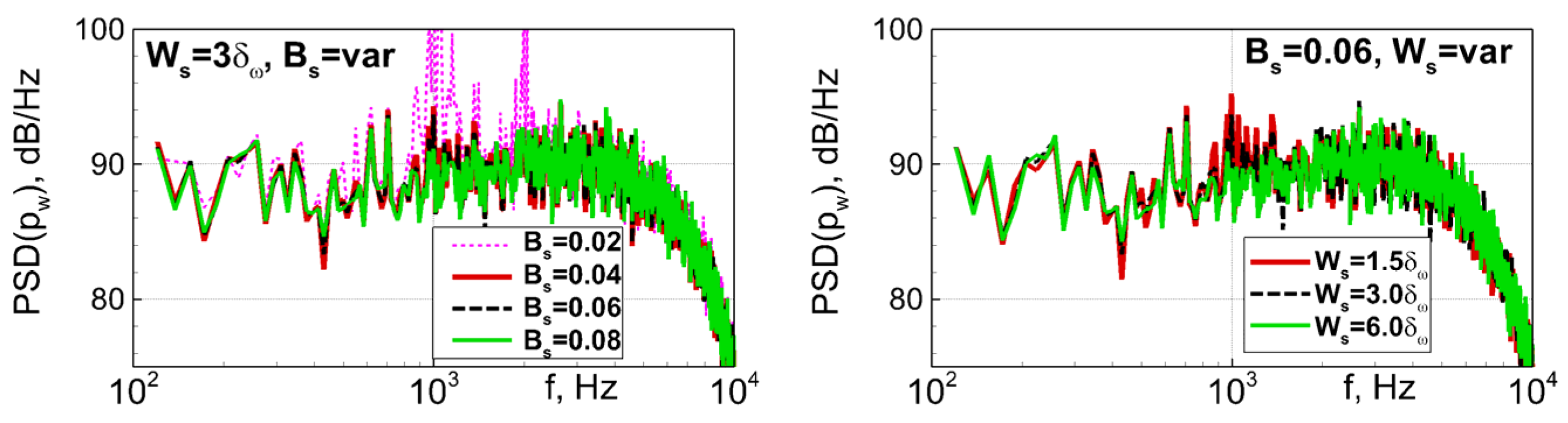
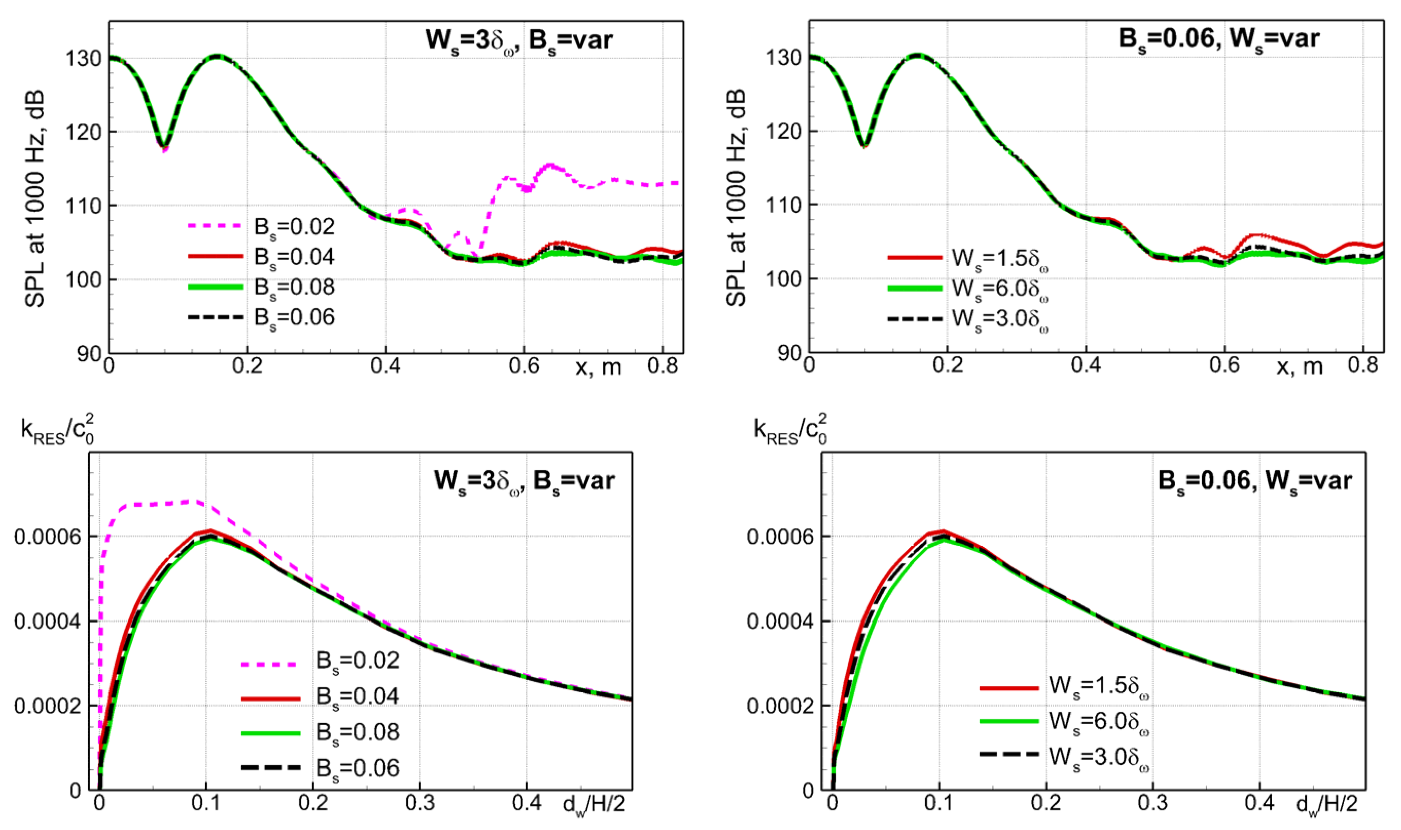
3.3. Calibration of the Body Force Parameters and Its Effect on Propagation of Sound Waves at Non-Resonant Frequencies

For tuning of the two parameters of the SRC2 source term (10), namely, the source width Ws and the amplitude factor Bs, we have used the NASA GIT experiment with CT57 liner [14] in the presence of external forcing at the near-resonant frequency fe = 1000 Hz. For this case, the WMLES [13] predicts the existence of hydrodynamic instability with a spatial growth rate much higher than that in the experiment (see [13] and Figure 1, Figure 2 and Figure 3 in Section 1). Therefore, this is the most suitable case for the calibration of the constants in the stabilization source term.
As far as the source width Ws is concerned, the inviscid origin of the hydrodynamic instability developing along the lined wall suggests that it should be scaled with the “vorticity thickness” of the near-wall velocity profile defined as δ ω = U e / | U / y | w , where U e is the boundary layer edge velocity (for the developed flow in a duct, it is replaced by the bulk velocity). In the course of the calibration, we varied the ratio W s / δ ω in the range 1.5 < W s / δ ω < 6 . For the GIT flow, this corresponds to the variation of W s from 0.005 up to 0.02 of the half-height of the duct. Thus, the region of non-zero source terms in all the considered cases was very narrow.
The amplitude factor Bs was varied from 0.02 up to 0.1, which values were deliberately chosen to be too small and too large, respectively.
The analysis of the results obtained in this series of computations suggests that the pair { W s = 3 δ ω , B s = 0.06 } can be considered an “optimal” compromise. It enables eliminating the instability in the considered flow, and thanks to this, it ensures a radically better agreement with the data [14] on the SPL distribution along the duct (see Figure 16, Figure 17 and Figure 18), with a marginal damping effect on the resolved turbulence (Figure 19) and virtually no effect on the mean flow characteristics, particularly the mean skin friction (Figure 20).
In addition, an encouraging result revealed by Figure 19 is that, similar to the case of the flow over the lined wall with no external acoustic signal considered in Section 3.2 above, a noticeable decrease of the velocity pulsations compared to those observed in the solid-wall duct takes place only in the very narrow area adjacent to the wall, d w < 0.05 ( H / 2 ) . Note that this remains so despite the increase in the amplitude factor Bs needed for the elimination of the instability in the case under consideration. As a result, the main part of the wall-normal profile of the TKE, including its near-wall maximum, is virtually unaffected by the damping source term.
One more positive property of the suggested clipped form of the source term SRC2 (10) is a relatively weak sensitivity of the results obtained with its use to the choice of both W s and B s : as seen in Figure 21, varying these parameters in a reasonably wide range around the optimal values, 1.5 δ ω < W s < 6 δ ω , 0.04 < B s < 0.08 , does not lead to any substantial alteration of the predictions.
We now turn to an evaluation of the side effect of the application of the stabilization body force (10), which consists of some errors introduced into the prediction of the propagation of the sound waves along the GIT at non-resonant frequencies because of distortion of the acoustic modes by the body force (see Table 1 above). For this purpose, the GIT flow [14] is computed at three frequencies of the external forcing by the plane acoustic waves, fe = 500 Hz, 1500 Hz, and 3000 Hz, covering the entire range of the frequency variation in the experiments (500 Hz < fe < 3000 Hz), with the stabilization body force (10) “turned on”. Its parameters were set as W s = 3 δ ω and B s = 0.06 , i.e., equal to the values just proven to enable elimination of the strong instability observed at the near-resonant forcing frequency. In Figure 22, corresponding SPL distributions along the lower wall of the GIT test section are compared with the similar distributions [13] obtained in the WMLES of the same cases carried out using the original (with no artificial source terms) governing equations and with the experiment [14].
The figure suggests that at all the forcing frequencies, the deterioration of the propagation of the sound waves caused by the introduction of the damping source term (10) is very weak: the difference between the SPL computed with this source term “turned on” and with the use of the non-modified equations is within 1 dB. The only exception is a part of the SPL-distribution at fe = 3000 Hz (Figure 22c) downstream of x = 0.5 m, where the sound wave intensity becomes so low that the computed SPLs are almost entirely defined by the “turbulent floor” of the wall-pressure pulsations.
We believe that the value of the ratio of the thickness of the non-zero source area Ws and the vorticity thickness at the lined wall δω chosen for the proposed stabilizing body force (10) based on the WMLES of the flow in the GIT with the CT57 liner ( W s / δ ω = 3 ) can be considered quite universal, i.e., can be used for suppressing the spatial instability in the scale-resolving simulations of flows over any other liners characterized by low acoustic resistance, when such instability may show up. As for the second parameter of the body force (the amplitude factor Bs), its minimum value ensuring elimination of the instability depends on the liner impedance and, therefore, should be adjusted to every specific liner. An example supporting these statements is presented in the next section.

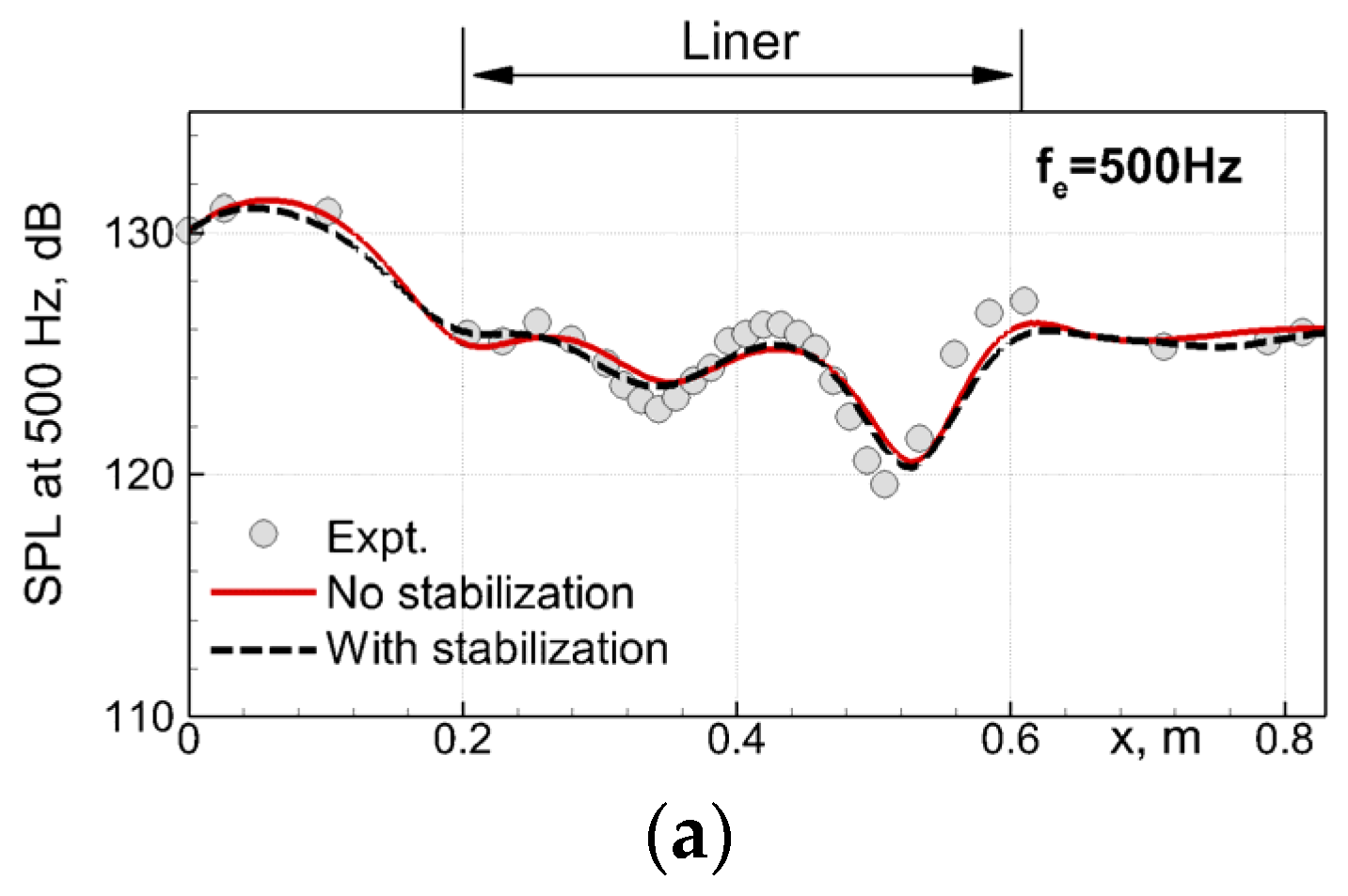
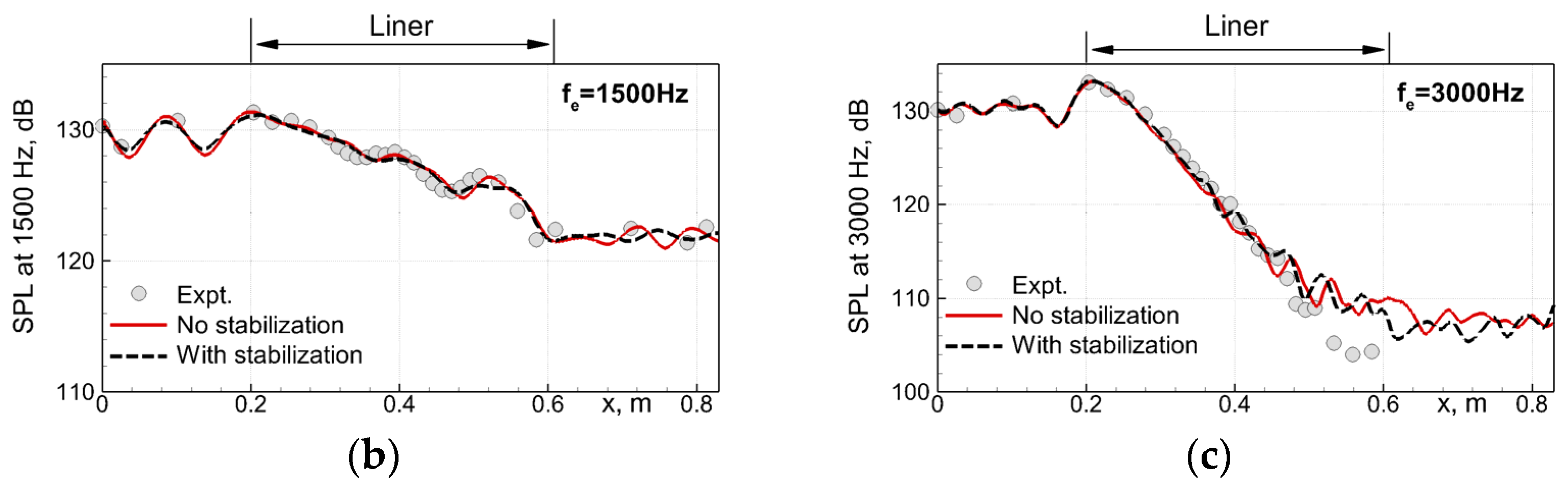
4. Application to an Alternative (SDoF) Liner

We consider the results of the scale-resolving simulations of the flow in the NASA GFIT [32] (see Section 2.1) with SDoF acoustic liner AE02, which, as mentioned earlier, is the “most unstable” one among a number of the SDoF liners tested in [32] and computed in [31] with the use of the URANS equations. The simulations of this flow are carried out at one of the frequencies of the external acoustic forcing from a wide range of experimental frequencies [32], namely, at fe = 1400 Hz. Judging by the URANS computations [31], in this flow, the hydrodynamic instability at the lined surface develops not only at the natural (resonant) frequency of the AE02 liner (fRES ≈ 1600 Hz), but simultaneously at the forcing frequency itself. For this reason, in terms of suppressing the instability in the simulations, this case is the most challenging one.
The simulations were performed at three different settings.
The first one employs the original governing equations, i.e., does not use any artificial source terms for suppressing the instability. A rapid development of a strong instability in this simulation, accompanied by the formation of pronounced large-scale vortical structures in the vicinity of the liner surface, is visually displayed by the flow visualization shown in Figure 23.
In the second simulation, in order to suppress the instability, the artificial body force (10) is used with the same parameters as those chosen in Section 3.3 for suppressing the instability in the computations of the GIT flow with the liner CT57, i.e., W s = 3 δ ω , B s = 0.06 .
The third simulation differs from the second only by the two-folds increased amplitude factor of the stabilizing body force, B s = 0.12 .
In addition, a simulation of the same flow in the absence of the liner sample (in the solid-wall duct) was carried out, which provides the target solution for the mean flow and the turbulent statistics.
Selected results from these simulations are presented in Figure 24, Figure 25, Figure 26, Figure 27 and Figure 28, where they are compared with each other and with the available experimental data [32]. Specifically, Figure 24 compares the instantaneous fields of the pressure fluctuations in a vertical plane of the duct, Figure 25 shows the streamwise evolution of the spectra of pressure at its upper (lined) wall, Figure 26 presents distributions of the sound pressure level at the considered forcing frequency along both duct walls, and Figure 27 and Figure 28 illustrate, respectively, the effect of the stabilizing source term on the turbulent fluctuations of velocity and on the mean skin friction coefficient.
The figures suggest that in the simulation of the GFIT flow over the AE02 liner with the use of the stabilizing body force and the amplitude factor B s = 0.06 , the hydrodynamic instability is still present, although its growth rate and amplitude are strongly reduced compared to those obtained in the simulation with the use of the original governing equations. This is not surprising, considering that the acoustic resistance of the AE02 liner at the resonant frequency is significantly (by a factor of ~1.5) smaller than that of the liner CT57 (see Figure 6 and Figure 7), for which the value B s = 0.06 was found optimal. However, the increase of B s up to 0.12 without changing the width parameter of the body force (10) does ensure virtually complete suppression of the instability, which is accompanied by a considerable improvement in the agreement of the predicted SPL(x) distribution with the measurements (see Figure 26). At the same time, as seen in Figure 27, this two-fold increase of the amplitude parameter versus the value used in the simulations of the flow over the CT57 liner does not lead to any noticeable additional contamination of the turbulent statistics caused by the stabilizing body force, which remains negligible, at least outside the very narrow ( d w < 0.05 ( H / 2 ) ) near-wall area. The same is true for the mean skin friction coefficient at the lined wall (see Figure 28).

5. Conclusions

This work deals with an issue arising in the turbulence-resolving simulations of the flows over the acoustic liners modelled in the framework of the macroscopic concept of the complex acoustic impedance. It consists in a strong overestimation of the growth rate of the spatial hydrodynamic instability developing along the liners having low acoustic resistance, which results in poor prediction of the propagation of the sound waves inside ducts with acoustically treated walls at the frequencies close to the liner resonant frequency.
A pragmatic approach to resolving this issue is adopted, which takes into account the experimental observation that in practical problems, the instability is either very weak or absent. Considering this, instead of an attempt to accurately reproduce the instability, it is artificially suppressed in the simulations by introducing specially designed volume source terms (body force) into the governing Navier–Stokes equations. Conceptually, the developed approach is similar to the approach recently suggested by Deng et al. [17] for the computations based on the linearized Euler equations. However, as shown in the current paper, their stabilizing source term is suboptimal for the scale-resolving simulations of turbulence because of a pronounced side effect of over-suppressing the turbulent fluctuations, whose correct prediction is essential for aeroacoustic problems.
A novel stabilizing body force proposed in the present work is designed based on the linear stability analysis and is tuned based on a wide set of numerical experiments, in which the flows in the grazing impedance tubes with two different liners are computed with the use of wall-modeled LES. It is shown that with the properly chosen body force parameters, the developed procedure is capable of eliminating the hydrodynamic instability with only a marginal impact on the prediction of the characteristics of the resolved turbulence. Particularly, the area of a discernible effect of the body force on the intensity of the turbulent fluctuations is confined by the very narrow (around 5% of the thickness of the boundary layer) zone adjacent to the lined surface. At the same time, it is less harmful to the acoustic modes than the body force [17]. As a result, the procedure ensures a drastic improvement in the accuracy of the computed sound attenuation by the liners at the near-resonant frequencies, with virtually no deterioration of the sound at other frequencies.
Another advantage of the developed approach is that the proposed form of the stabilizing body force is fairly versatile. For the computation of the flow over a specific liner, a user has to adjust only one parameter (the amplitude factor Bs), whose optimal value depends upon the liner impedance at the resonant sound frequency. This task is facilitated by the weak sensitivity of predictions to an increase in Bs versus its minimum value, ensuring a complete suppression of the hydrodynamic instability.

Author Contributions

Conceptualization, M.S. (Mikhail Shur) and M.S. (Mikhail Strelets); methodology, M.S. (Mikhail Shur) and A.T.; software, A.T.; validation, M.S. (Mikhail Shur) and A.T.; investigation, M.S. (Mikhail Shur) and A.T.; writing—original draft preparation, M.S. (Mikhail Shur); writing—review and editing, M.S. (Mikhail Strelets) and M.S. (Mikhail Shur); visualization, A.T.; supervision, M.S. (Mikhail Strelets); project administration, M.S. (Mikhail Strelets). All authors have read and agreed to the published version of the manuscript.

Funding

This research was funded by the Ministry of Science and Higher Education of the Russian Federation as part of the World-class Research Center program: Advanced Digital Technologies (contract no. 075-15-2022-311 dated 20 April 2022).

Data Availability Statement

The results of the simulations presented in this study are available from the corresponding author on reasonable request.

Acknowledgments

The authors greatly appreciate the help of and fruitful discussions with Takao Suzuki. All the computations were conducted with the use of the HP computing facilities of the Peter the Great Saint-Petersburg Polytechnic University (http://www.spbstu.ru; accessed on 11 April 2023).

Conflicts of Interest

The authors declare no conflict of interest.

References

  1. Eversman, W. Theoretical Models for Duct Acoustic Propagation and Radiation. In Aeroacoustics of Flight Vehicles: Theory and Practice, Noise Control; NASA RP-1258; NASA Langley Research Center: Hampton, VA, USA, 1991; Volume 2, pp. 101–163. [Google Scholar]
  2. Motsinger, R.E.; Kraft, R.E. Design and Performance of Duct Acoustic Treatment. In Aeroacoustics of Flight Vehicles: Theory and Practice, Noise Control; NASA RP-1258; NASA Langley Research Center: Hampton, VA, USA, 1991; Volume 2, pp. 165–206. [Google Scholar]
  3. Rienstra, S.W.; Hirschberg, A. An Introduction to Acoustics. Ph.D. Thesis, Eindhoven University of Technology, Eindhoven, The Netherlands, 2019. [Google Scholar]
  4. Myers, M.K. On the Acoustic Boundary Condition in the Presence of Flow. J. Sound Vib. 1980, 71, 429–434. [Google Scholar] [CrossRef]
  5. Rienstra, S.W. Impedance Models in Time Domain, Including the Extended Helmholtz Resonator Model. In Proceedings of the 12th AIAA/CEAS Aeroacoustics Conference, Cambridge, MA, USA, 8–10 May 2006; AIAA Paper: Cambridge, MA, USA, 2006; p. 2686. [Google Scholar] [CrossRef]
  6. Tam, C.K.W.; Auriault, L. Time-Domain Impedance Boundary Conditions for Computational Aeroacoustics. AIAA J. 1996, 34, 917–923. [Google Scholar] [CrossRef]
  7. Reymen, Y.; Baelmans, M.; Desmet, W. Efficient Implementation of Tam and Auriault’s Time-Domain Impedance Boundary Condition. AIAA J. 2008, 46, 2368–2376. [Google Scholar] [CrossRef]
  8. Li, X.Y.; Li, X.D.; Tam, C.K.W. Improved Multipole Broadband Time-Domain Impedance Boundary Condition. AIAA J. 2012, 50, 980–984. [Google Scholar] [CrossRef]
  9. Ozyoruk, Y.; Long, L.N.; Jones, M.G. Time-Domain Numerical Simulation of a Flow-Impedance Tube. J. Comp. Phys. 1998, 146, 29–57. [Google Scholar] [CrossRef]
  10. Fung, K.-Y.; Ju, H. Broadband Time-Domain Impedance Models. AIAA J. 2001, 39, 1449–1454. [Google Scholar] [CrossRef]
  11. Dragna, D.; Pineau, P.; Blanc-Benon, P. A Generalized Recursive Convolution Method for Time-Domain Propagation in Porous Media. J. Acoust. Soc. Amer. 2015, 138, 1030–1042. [Google Scholar] [CrossRef]
  12. Troian, R.; Dragna, D.; Bailly, C.; Galland, M.-A. Broadband Liner Impedance Eduction for Multimodal Acoustic Propagation in the Presence of a Mean Flow. J. Sound Vib. 2017, 392, 200–216. [Google Scholar] [CrossRef]
  13. Shur, M.; Strelets, M.; Travin, A.; Suzuki, T.; Spalart, P. Unsteady Simulations of Sound Propagation in Turbulent Flow Inside a Lined Duct. AIAA J. 2021, 59, 3054–3070. [Google Scholar] [CrossRef]
  14. Jones, M.G.; Watson, W.R.; Parrott, T.L. Benchmark Data for Evaluation of Aeroacoustic Propagation Codes with Grazing Flow. In Proceedings of the 11th AIAA/CEAS Aeroacoustics Conference, Monterey, CA, USA, 23–25 May 2005; AIAA Paper: Monterey, CA, USA, 2005; p. 2853. [Google Scholar] [CrossRef]
  15. Shur, M.L.; Spalart, P.R.; Strelets, M.K.; Travin, A.K. A Hybrid RANS-LES Approach with Delayed-DES and Wall-Modelled LES Capabilities. Int. J. Heat Fluid Flow 2008, 29, 1638–1649. [Google Scholar] [CrossRef]
  16. Rienstra, S.W.; Vilenski, G.G. Spatial Instability of Boundary Layer Along Impedance Wall. In Proceedings of the 14th AIAA/CEAS Aeroacoustics Conference, Vancouver, BC, Canada, 5–7 May 2008; AIAA Paper: Vancouver, BC Canada, 2008; p. 2932. [Google Scholar] [CrossRef]
  17. Deng, Y.; Alomar, A.; Dragna, D.; Galland, M.-A. Characterization and Suppression of the Hydrodynamic Instability in the Time Domain for Acoustic Propagation in a Lined Flow Duct. J. Sound Vib. 2021, 500, 115999. [Google Scholar] [CrossRef]
  18. Dai, X.; Auregan, Y. A Cavity-by-Cavity Description of the Aeroacoustic Instability Over a Liner with a Grazing Flow. J. Fluid Mech. 2018, 852, 126–145. [Google Scholar] [CrossRef]
  19. Marx, D.; Auregan, Y.; Bailliet, H.; Valiere, J.-C. PIV and LDV Evidence of Hydrodynamic Instability over a Liner in a Duct Flow. J. Sound Vib. 2010, 329, 3798–3812. [Google Scholar] [CrossRef]
  20. Marx, D. Numerical Computation of a Lined Duct Instability Using the Linearized Euler Equations. AIAA J. 2015, 53, 2379–2388. [Google Scholar] [CrossRef]
  21. Rienstra, S.W.; Darau, M. Boundary-Layer Thickness Effects of the Hydrodynamic Instability along an Impedance Wall. J. Fluid Mech. 2011, 671, 559–573. [Google Scholar] [CrossRef]
  22. Dai, X.; Auregan, Y. Hydrodynamic Instability and Sound Amplification Over a Perforated Plate Backed by a Cavity. In Proceedings of the 25th AIAA/CEAS Aeroacoustics Conference, Delft, The Netherlands, 20–23 May 2019; AIAA Paper: Delft, The Netherlands, 2019; p. 2703. [Google Scholar] [CrossRef]
  23. Marx, D.; Sebastian, R.; Fortune, V. Spatial Numerical Simulation of a Turbulent Plane Channel Flow with an Impedance Wall. In Proceedings of the 25th AIAA/CEAS Aeroacoustics Conference, Delft, The Netherlands, 20–23 May 2019; AIAA Paper: Delft, The Netherlands, 2019; p. 2543. [Google Scholar] [CrossRef]
  24. Shur, M.; Strelets, M.; Travin, A.; Suzuki, T.; Spalart, P.R. Unsteady Simulation of Sound Propagation in Turbulent Flow Inside a Lined Duct Using a Broadband Time-Domain Impedance Model. In Proceedings of the AIAA Aviation 2020 Forum Virtual Event, Virtual, 15–19 June 2020; AIAA Paper: Delft, The Netherlands, 2020; p. 2535. [Google Scholar] [CrossRef]
  25. Marx, D.; Auregan, Y. Effect of Turbulent Eddy Viscosity on the Unstable Surface Mode above an Acoustic Liner. J. Sound Vib. 2013, 332, 3803–3820. [Google Scholar] [CrossRef]
  26. Sebastien, R.; Marx, D.; Fortune, V. Numerical Simulation of a Turbulent Channel Flow with an Acoustic Liner. J. Sound Vib. 2019, 456, 306–330. [Google Scholar] [CrossRef]
  27. Richter, C.; Thiele, F.H.; Li, X.; Zhuang, M. Comparison of Time-Domain Impedance Boundary Conditions for Lined Duct Flows. AIAA J. 2007, 45, 1333–1345. [Google Scholar] [CrossRef]
  28. Burak, M.O.; Billson, M.; Eriksson, L.-E.; Baralon, S. Validation of a Time- and Frequency-Domain Grazing Flow Acoustic Liner Model. AIAA J. 2009, 47, 1841–1848. [Google Scholar] [CrossRef]
  29. Deng, Y.; Dragna, D.; Galland, M.-A.; Alomar, A. Comparison of Three Numerical Methods for Acoustic Propagation in a Lined Duct with Flow. In Proceedings of the 25th AIAA/CEAS Aeroacoustics Conference, Delft, The Netherlands, 20–23 May 2019; AIAA Paper: Delft, The Netherlands, 2019; p. 2658. [Google Scholar] [CrossRef]
  30. Bogey, C.; Bailly, C.; Juve, D. Computation of Flow Noise Using Source Terms in Linearized Euler’s Equations. AIAA J. 2002, 40, 235–243. [Google Scholar] [CrossRef]
  31. Shur, M.; Strelets, M.; Travin, A.; Suzuki, T. Further Evaluation of Prediction Capability of the Broadband Time-Domain Impedance Model for Sound Propagation in Turbulent Grazing Flow. In Proceedings of the AIAA Aviation 2021 Forum Virtual Event, Virtual, 2–6 August 2021; AIAA Paper: Delft, The Netherlands, 2021; p. 2171. [Google Scholar] [CrossRef]
  32. Howerton, B.M.; Jones, M.G. A Conventional Liner Acoustic/Drag Interaction Benchmark Database. In Proceedings of the 23rd AIAA/CEAS Aeroacoustics Conference, Denver, CO, USA, 5–9 June 2017; AIAA Paper: Denver, CO, USA, 2017; p. 4190. [Google Scholar] [CrossRef]
  33. Zheng, S.; Zhuang, M. Verification and Validation of Time-Domain Impedance Boundary Condition in Lined Ducts. AIAA J. 2005, 43, 306–313. [Google Scholar] [CrossRef]
  34. Parrott, T.L.; Watson, W.R.; Jones, M.G. Experimental Validation of a Two-Dimensional Shear-Flow Model for Determining Acoustic Impedance; NASA TP: Washington, DC, USA, 1987; p. 2679. [Google Scholar]
  35. Shur, M.; Strelets, M.; Travin, A.; Probst, A.; Probst, S.; Schwamborn, D.; Deck, S.; Skillen, A.; Holgate, J.; Revell, A. Improved Embedded Approaches. In Go4Hybrid: Grey Area Mitigation for Hybrid RANS-LES Methods, Notes on Numerical Fluid Mechanics and Multidisciplinary Design; Springer: New York, NY, USA, 2017; Volume 134, pp. 51–87. [Google Scholar] [CrossRef]
  36. Shur, M.L.; Spalart, P.R.; Strelets, M.K. Noise prediction for increasingly complex jets. Part 1: Methods and tests. Int. J. Aeroacoustics 2005, 4, 213–245. [Google Scholar] [CrossRef]
  37. Gustavsen, B.; Semlyen, A. Rational Approximation of Frequency Domain Responses by Vector Fitting. IEEE Trans. Power Deliv. 1999, 14, 1052–1061. [Google Scholar] [CrossRef]
  38. Gustavsen, B. Improving the Pole Relocating Properties of Vector Fitting. IEEE Trans. Power Deliv. 2006, 21, 1587–1592. [Google Scholar] [CrossRef]
  39. Deschrijver, D.; Mrozowski, M.; Dhaene, T.; De Zutter, D. Macromodeling of Multiport Systems Using a Fast Implementation of the Vector Fitting Method. IEEE Microw. Wirel. Compon. Lett. 2008, 18, 383–385. [Google Scholar] [CrossRef]
  40. Zhang, Q.; Bodony, D.J. Numerical Investigation of a Honeycomb Liner Grazed by Laminar and Turbulent Boundary Layers. J. Fluid Mech. 2016, 792, 936–980. [Google Scholar] [CrossRef]
  41. Leon, O.; Mery, F.; Piot, E.; Conte, C. Near-wall Aerodynamic Response of an Acoustic Liner to Harmonic Excitation with Grazing Flow. Exp. Fluid 2019, 60, 144. [Google Scholar] [CrossRef]
  42. Qui, X.; Xin, B.; Wu, L.; Meng, Y.; Jing, X. Investigation of Straightforward Impedance Eduction Method on Single-Degree-of-Freedom Acoustic Liners. Chin. J. Aeronaut. 2018, 31, 2221–2233. [Google Scholar] [CrossRef]
  43. Shur, M.; Strelets, M.; Travin, A. High-order Implicit Multi-block Navier-Stokes Code: Ten-year Experience of Application to RANS/DES/LES/DNS of Turbulent Flows. In Proceedings of the 7th Symposium on Overset Composite Grids & Solution Technology, Huntington Beach, CA, USA; 2004. Available online: https://cfd.spbstu.ru//agarbaruk/doc/NTS_code.pdf (accessed on 11 April 2023).
  44. Roe, P.L. Approximate Riemann Solvers, Parameter Vectors and Difference Schemes. J. Comput. Phys. 1981, 43, 357–372. [Google Scholar] [CrossRef]
  45. Howerton, B.M.; Jones, M.G. Acoustic Liner Drag: Measurements on Novel Facesheet Perforate Geometries. In Proceedings of the 22nd AIAA/CEAS Aeroacoustics Conference, Lyon, France, 30 May–1 June 2016; AIAA Paper: Lyon, France, 2016; p. 2979. [Google Scholar] [CrossRef]
  46. Spalart, P.R.; Garbaruk, A.V.; Howerton, B.M. CFD Analysis of an Installation Used to Measure the Skin-Friction Penalty of Acoustic Treatments. In Proceedings of the 23rd AIAA/CEAS Aeroacoustics Conference, Denver, CO, USA, 5–9 June 2017; AIAA Paper: Denver, CO, USA, 2017; p. 3691. [Google Scholar] [CrossRef]
Figure 1. WMLES predictions [13] of the effect of liner and acoustic forcing on instantaneous fields of vorticity magnitude in a meridian plane and at the upper (lined) wall and pressure fluctuations in a meridian plane of NASA GIT [14] (liner shown by grey rectangular is located at 0.2 m < x < 0.61 m). (a): flow in solid-wall duct (no liner); (b): flow in duct with liner and acoustic forcing at fe = 1000 Hz; (c): flow in duct with liner without any external forcing.
Fluids 08 00134 g001
Figure 2. Effect of liner and acoustic forcing on the wall-pressure spectrum at a location close to liner’s downstream edge (a) and mean skin-friction distribution along duct upper wall (b) predicted by WMLES [13]. Green line: solid-wall duct (no liner); red: duct with liner and external forcing by plane sound waves of intensity 130 dB at fe = 1000 Hz; blue: duct with liner and without any external forcing.
Fluids 08 00134 g002
Figure 3. Measured in [14] and predicted by WMLES [13] distributions of sound pressure level along upper (with the liner) and lower (opposite to the liner) walls of NASA GIT at fe = 1000 Hz.
Fluids 08 00134 g003
Figure 4. Schematics of NASA GIT [14] test section (a) and of NASA GFIT [32] flow path (b).
Fluids 08 00134 g004
Figure 5. Schematic of XY-cut of the computational domain used in zonal RANS-IDDES showing locations of the VSTG and the exit sponge layer together with an example of an instantaneous field of vorticity magnitude.
Fluids 08 00134 g005
Figure 6. Frequency-dependence of acoustic resistance R and reactance X of the CT57 liner from experiment [14] and its VF-approximation by multipole function.
Fluids 08 00134 g006
Figure 7. Acoustic resistance and reactance of AE02 liner at MAV = 0.4 and different levels of wall-pressure fluctuations.
Fluids 08 00134 g007
Figure 8. Instantaneous fields of vorticity magnitude at the upper (lined) wall and pressure fluctuations in a meridian plane from WMLES of the flow in the GIT without external acoustic signal with the use of stabilization body force SRC1 (7) at BD = 0.4. Compare these fields with the corresponding fields in Figure 1a,c.
Fluids 08 00134 g008
Figure 9. Instantaneous fields of fluctuations of vertical (normal to the lined wall) velocity at x = 0.6 m from WMLES of flows in the duct with solid walls using original governing equations (a) and in the duct with liner using equations with added stabilization body force SRC1 (7) at BD = 0.4 (b).
Fluids 08 00134 g009
Figure 10. Comparison of wall-pressure spectra at x = 0.6 m predicted by WMLES of three flows. Green: duct with solid walls, original equations; red: duct with liner, original equations; blue: duct with liner, equations with added stabilization body force SRC1 (7) at BD = 0.4.
Fluids 08 00134 g010
Figure 11. Same as in Figure 10, for streamwise distributions of root-mean-square wall-pressure fluctuations (a) and mean friction coefficient (b).
Fluids 08 00134 g011
Figure 12. Comparison of wall-normal profiles of root-mean-square pulsations of velocity components and resolved TKE at x = 0.6 m predicted by the three WMLES.
Fluids 08 00134 g012
Figure 13. Comparison of wall-normal profiles of root-mean-square pulsations of velocity components and resolved TKE at x = 0.6 m from simulations of flows in the solid-wall duct using original governing equations; in the duct with liner using equations with added stabilization body force SRC1 (7) at BD = 0.4; and in the duct with liner using equations with added stabilization body force SRC2 (9) at Bs = 0.02.
Fluids 08 00134 g013
Figure 14. Same as in Figure 13, for wall-pressure spectra at x = 0.6 m (a) and streamwise distributions of root-mean-square wall-pressure pulsations (b) and mean friction coefficient (c).
Fluids 08 00134 g014
Figure 15. Comparison of wall-normal profiles of resolved TKE at x = 0.6 m predicted for solid-wall duct using original governing equations and for lined duct using equations with added clipped stabilizing body force SRC2 (10).
Fluids 08 00134 g015
Figure 16. Instantaneous field of pressure fluctuations in a vertical plane XY from simulation of NASA GIT flow at fe = 1000 Hz using optimal ( W s = 3 δ ω , B s = 0.06 ) stabilization source term (10). Compare this field with similar field from WMLES without stabilization in Figure 1b.
Fluids 08 00134 g016
Figure 17. Effect of stabilization (10) with optimal parameters on downstream evolution of pressure spectra at the lined wall for NASA GIT flow at fe = 1000 Hz. Red line: computation without stabilization [13]; black: with stabilization; green: flow in solid-wall duct.
Fluids 08 00134 g017
Figure 18. Effect of stabilization (10) with optimal parameters on SPL-distribution along lower (a) and upper (b) walls of GIT.
Fluids 08 00134 g018
Figure 19. Effect of stabilization (10) with optimal parameters on wall-normal profiles of root-mean-square pulsations of velocity and resolved TKE at x = 0.6 m.
Fluids 08 00134 g019
Figure 20. Effect of stabilization (10) with optimal parameters on skin-friction at lined wall of GIT.
Fluids 08 00134 g020
Figure 21. Sensitivity of predictions of NASA GIT flow at fe = 1000 Hz to parameters Bs and Ws of stabilization body force (10). Upper row: spectra of wall-pressure fluctuations at x = 0.6 m; mid row: SPL at the lower wall; lower row: profiles of resolved TKE at x = 0.6 m.
Fluids 08 00134 g021aFluids 08 00134 g021b
Figure 22. Effect of stabilization (10) on computed SPL distributions along the GIT wall at non-resonant forcing frequencies. (a): fe = 500 Hz; (b): 1500 Hz; (c): 3000 Hz.
Fluids 08 00134 g022aFluids 08 00134 g022b
Figure 23. Instantaneous iso-surface of swirl parameter (magnitude of the second eigenvalue of the velocity gradient tensor) λ 2 = 10 c 0 / ( H / 2 ) from the simulation of the flow in NASA GFIT with AE02 liner using the original governing equations. The iso-surface is “colored” by local value of streamwise velocity component.
Fluids 08 00134 g023
Figure 24. Effect of stabilization (10) and its amplitude parameter Bs on instantaneous field of pressure fluctuations in a vertical plane of NASA GFIT flow. Location of AE02 SDoF liner on the upper wall is shown by the grey rectangular.
Fluids 08 00134 g024
Figure 25. Effect of stabilization (10) and its amplitude parameter Bs on the evolution of wall pressure spectra at the upper (lined) wall of NASA GFIT.
Fluids 08 00134 g025
Figure 26. Effect of stabilization (10) and its amplitude parameter Bs on distributions of SPL along lower and upper walls of NASA GFIT.
Fluids 08 00134 g026
Figure 27. Effect of stabilization (10) and its amplitude parameter Bs on wall-normal profiles of root-mean-square pulsations of velocity and resolved TKE at section x = 0.6 m of NASA GFIT flow.
Fluids 08 00134 g027
Figure 28. Effect of stabilization (10) and its amplitude parameter Bs on mean skin-friction coefficient at upper wall of NASA GFIT.
Fluids 08 00134 g028
Table 1. LSA predictions of acoustic complex eigenvalues kx for original Navier-Stokes equations and equations with added stabilization source terms SRC1 (7) and SRC2 (9).
f, Hzk1k2
Unchanged
Equations
with
SRC1
with
SRC2
Unchanged
Equations
with
SRC1
with
SRC2
5000.235 + 0.020i0.242 + 0.021i0.238 + 0.023i−0.642 − 0.114i−0.593 − 0.096i−0.621 − 0.100i
10000.432 + 0.281i0.431 + 0.323i0.427 + 0.295i−0.406 − 0.486i−0.432 − 0.478i−0.415 − 0.489i
15000.449 + 0.058i0.443 + 0.062i0.447 + 0.058i−0.863 − 0.110i−0.877 − 0.103i−0.868 − 0.111i
Disclaimer/Publisher’s Note: The statements, opinions and data contained in all publications are solely those of the individual author(s) and contributor(s) and not of MDPI and/or the editor(s). MDPI and/or the editor(s) disclaim responsibility for any injury to people or property resulting from any ideas, methods, instructions or products referred to in the content.

