
PIV Measurements of Open-Channel Turbulent Flow under Unconstrained Conditions

Department of Mechanical Engineering, Bucknell University, Lewisburg, PA 17837, USA
Fluids 2023, 8(4), 135; https://doi.org/10.3390/fluids8040135
Submission received: 13 March 2023
/
Revised: 4 April 2023
/
Accepted: 12 April 2023
/
Published: 18 April 2023
(This article belongs to the Special Issue Turbulent Flow, 2nd Edition)
Abstract
:Many open-channel turbulent flow studies have been focused on highly constrained conditions. Thus, it is rather conventional to note such flows as being fully developed, fully turbulent, and unaffected by sidewalls and free surface disturbances. However, many real-life flow phenomena in natural water bodies and artificially installed drain channels are not as ideal. This work is aimed at studying some of these unconstrained conditions. This is achieved by using particle image velocimetry measurements of a developing turbulent open-channel flow over a smooth wall. The tested flow effects are low values of the Reynolds number based on the momentum thickness (ranging from 165 to 930), low aspect ratio AR (ranging from 1.1 to 1.5), and Froude number Fr (ranging from 0.1 to 0.8). The results show that the mean flow has an inner region with a logarithmic layer with a von Kármán constant of 0.40–0.41, and a log law constant ranging from 5.0 to 6.0. The friction velocity and coefficient of skin friction are predictable using the formulations of Fr and presented in this work. The outer region is also characterized by a dip location, which is predictable using an equation associated with . The higher-order turbulence statistics, on the other hand, show distinguishing traits, such as correlation coefficients ranging from −0.1 to 0.5. Overall, this work demonstrates that for the unconstrained conditions studied, friction evaluations associated with Reynolds shear stress and some notable turbulence modelling functions used in conventional open-channel flows are inapplicable.
1. Introduction
Turbulent flows in open-channels are observed in many applications, ranging from natural water bodies to artificially installed drains. While some of the general outlines of the flow may be inferred from a theoretical knowledge of classical turbulent boundary layers, the flow is in many ways much more complex. This is especially so, given the nature and prevalence of bed conditions, sidewall confinements, and free surface effects. Consequently, as noted by Nezu [1], several studies have been conducted over several decades to understand the flow phenomena. This work focuses on turbulent open-channel flows over smooth walls.
In view of the shear complexity of the flow, experimental research has been far more valuable in establishing many of the fundamental features of turbulent flow in open-channel arrangements. This has been made possible through the use of measurement techniques, such as total head (or Pitot) tubes, propeller current meters, H2-bubble, hot-film anemometry, laser Doppler anemometry (LDA), and acoustic Doppler velocimetry (ADV). From such tests, several observations about the turbulent boundary layer structure have been established [2]. Accordingly, we know that the mean streamwise velocity profile of the turbulent flow in the mid-span consists of an inner region (close to the bed), and an outer region (further away from the bed). The inner region is also subdivided into a viscous sublayer directly adjacent to the bed where viscous forces are dominant, an intermediate region of transition called the buffer layer, and a fully developed turbulent region where a universal log law applies. In the outer region, the effects of the flow depth are prominent. In this zone, the velocity defect profiles tend to be parabolic, and the maximum observed value is a “dip” below the free surface. A substantial body of the works in this subject area have been focused on assessing the bed friction parameters and scaling laws, and developing predictive formulations to forecast flow parameters and profiles [3,4,5,6]. These often emanate from single-point turbulence statistics.
It is worth noting however that many of the concrete observations associated with turbulent open-channel flows have been based on highly constrained flow set-ups. As such, it is customary to see data extracted from fully developed regions of the turbulent flow field, and for conditions where sidewall effects (in the form of secondary currents) and surface disturbances are minimal. Nonetheless, it must be conceded that many real-life flow phenomena are far from such idealized constraints. They may, for example, be subjected to sudden interruptions or short conduit paths that may lead to an undeveloped flow condition at the location of interest. They may also be under extremely low currents such that the local Reynolds number could be considerably low. Additionally, flows may experience extreme confinements, narrow channeling, and wave velocities arising from disturbances such that the sidewall and surface effects cannot be ignored.
Taking the aforementioned possibilities into account, some researchers have studied the flow phenomena under less constrained conditions. Sarma et al. [2], for instance, carried out a wide-ranged experimental program to characterize the flow when the channel aspect ratio (AR, which is the ratio of width to flow depth) varied from 1.0 to 8.0 and the Froude number (Fr) varied from 0.2 to 0.7. As their data were obtained from Pitot-static tube measurements, they only considered mean (streamwise) velocity distribution. Subsequently, they concluded that Fr and AR had no significant bearing on the form of the equation for the fully developed velocity distribution in the outer region of the sidewall close to the bed. Later, Kirkgöz and Ardiclioglu [7] studied the flow for both developing and developed flows, while accounting for sidewall effects. From their LDA measurements, they were able to observe that the inner layer of the developing flow also conformed to the logarithmic law. However, they pointed out that boundary layer along the channel mid-span develops up to the free surface if the flow AR was equal to three. In order to evaluate the lower limit of turbulence, Balachandar and Ramachandran [3] also conducted an extensive set of LDA measurements for flow conditions of a momentum Reynolds number (Reθ) ranging from 180 to 480. Their tests confirmed the existence of a fully developed turbulent boundary layer even under such a low range of Reθ. This is in stark contrast with the “often quoted lowest estimate of 320” [3]. More recently, Sarkar [8] and Mahananda et al. [9,10] used ADV to measure the flow in an open-channel flow of a low aspect ratio (i.e., AR > 2). Of the studies briefly covered in this paragraph, these works stand out as they are the only ones that have investigated something more than the mean velocity data. The detailed assessments of Sarkar [8] shows that the turbulent bursting within the dip of the outer flow showed that the non-dimensional Reynolds shear stress changes its sign from positive to negative within the dip. Mahananda et al. [9,10], on the other hand, discovered that the AR and Reynolds number affect the velocity characteristics in the developing region. However, these works only provide single-point measurements and they do not consider the influence of Fr.
Thus, in more general terms, while the current knowledge base is significant, it is limited in two major ways. Firstly, a large proportion of the literature concerning open-channel turbulent flow has been based on model conditions that do not account for the possibility of an undeveloped flow, sidewall effects, surface disturbances, and a low Reynolds number. Consequently, while the study of flows under unconstrained conditions exists, it is far from the normal stream of research focus, and it requires further consideration. Secondly, the current information in the literature is largely backed by data emanating from single-point measurement techniques, and far less comes from whole flow field measurements. Thus, many studies lack the full picture of detailed multidirectional field snapshots of measurement.
To help furnish the above-mentioned short-falls in the literature, the goal of this work is to investigate turbulent open-channel flows under relatively unconstrained conditions. What sets this work apart from other studies is that while other works are usually limited to one or two unconstrained conditions, this work aims to consider a much wider range of unconstrained conditions, namely, a non-developed flow, a low Reynolds number, a low AR channel, and a low to near-critical Fr. In particular, to the author’s knowledge, the lower limits of the Reynolds number and AR conditions explored in this work are the lowest recorded in the literature for measurements extracted from flows that are not fully developed. Indeed, the detailed whole flow field velocity measurements provided through the planar particle image velocimetry technique for such flow conditions are apparently non-existent in the literature. Therefore, with such unique measurements, this work aims to add significant contributions to the database in the literature by (1) characterizing the effects of aspect ratio, Reynolds number, and Froude number of a narrow open-channel turbulent flow that is not fully developed; (2) providing ways to predict essential parameters; and (3) determining how the flow features compare with fully developed open-channel flows.
2. Experimental System and Measurement Procedure
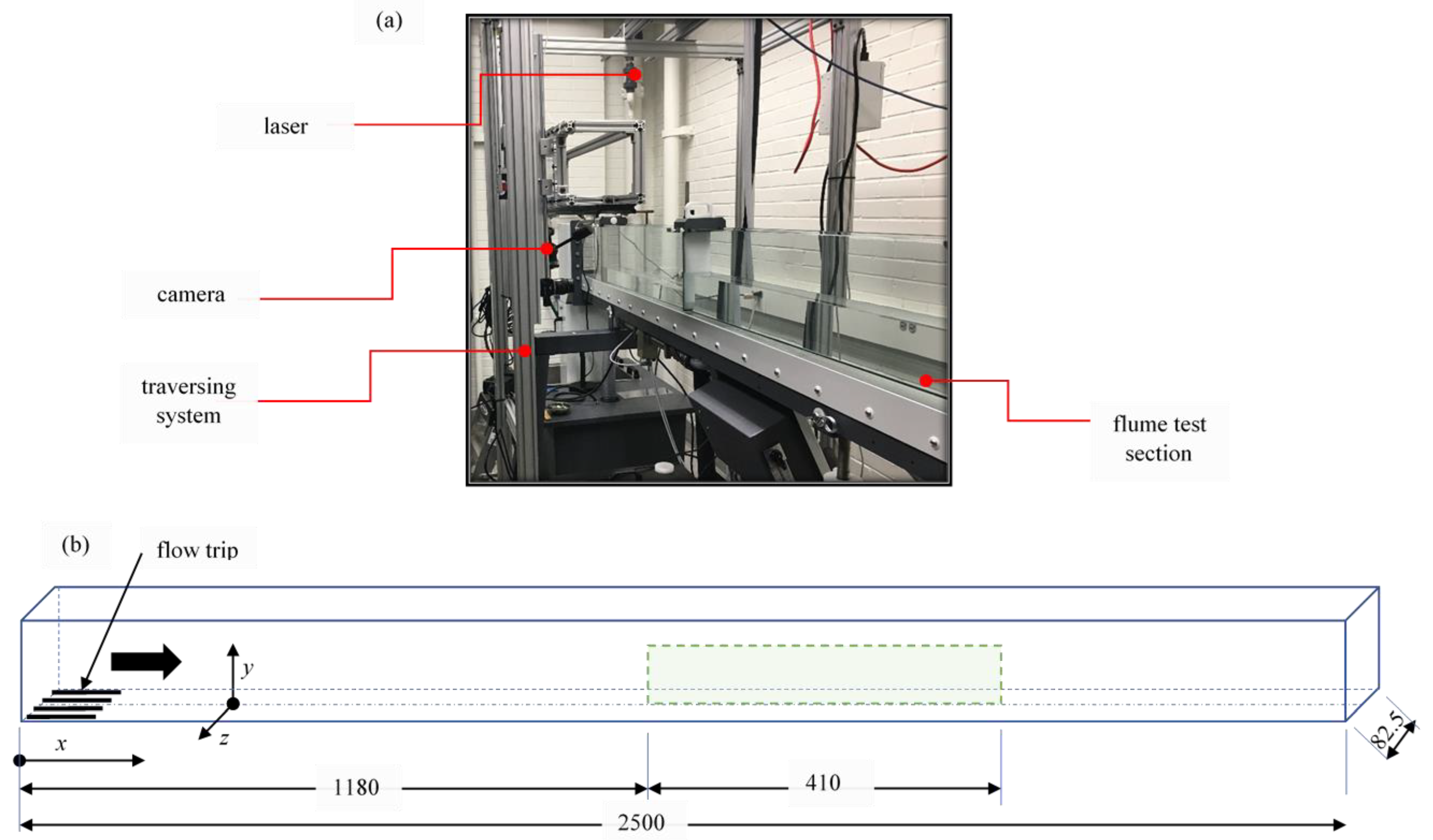
The experiments were conducted at Bucknell University’s Fluid Flow and Experimental Research Laboratory, USA. The experimental set-up consisted of a flume and a particle image velocimetry system. A schematic diagram of the arrangement of the experimental system is shown in Figure 1.
The flume used in this work is an open flow transport channel having a test section of rectangular cross-section. The test section is equipped with transparent acrylic walls, and of approximate dimensions of length L = 2.5 m, width b = 0.08 m, and depth H = 0.25 m. The system works in a closed recirculation, pumping water from a reservoir through a flow conditioner to the test section, and then back to the reservoir [11]. For the purpose of this research, certain modifications were made to the channel. The flow development of the turbulent boundary layer was enhanced using a triad of 9 mm-diameter rods fixed at the entry to the test section to serve as trips. In order to reduce reflection during velocity measurements, a dark polyvinyl chloride (PVC) plate was glued onto the bottom wall of the flume. This plate provided the smooth bed surface required for the tests. By utilizing a gate close to the exit of the test section, various depths of flow (55 mm< h < 75 mm) were achieved at a constant bed slope. This ensured that the aspect ratio (AR = b/h) of the channel flow was sufficiently low, thus maintaining a narrow channel condition (i.e., AR < 5 [1]) throughout the testing process. As shown in Figure 1, the coordinate system adopted in this work is fixed relative to the flume. The directions x, y, and z represent the directions along the stream, wall-normal, and the span, respectively. The origin of the coordinate system is specified such that x = 0 is fixed at the entrance into the test section of the flume, and y = 0 and z = 0 are, respectively, on top of the PVC plate and in the mid-span of the channel.
Velocity measurements were obtained using a planar particle image velocimetry (PIV) system entailing a laser, camera, programable timing unit, and a computer. As each of these PIV components utilized in this work is identical to that described in a previous publication [12], details regarding specifications will not be repeated here. However, it is important to note that for this work, the camera body was attached to a 28 mm focal length Nikkor lens. The camera assembly was in turn fitted with an orange filter with a band-pass wavelength of 532 nm ± 10 nm. For the PIV system, the laser and the camera were attached to a translation stage. In this way, both could be traversed as a unit in the streamwise direction without changing the distance between them. The flow was seeded with silver-coated hollow glass spheres with a mean diameter of 10 μm and a specific gravity of 1.4. Velocity measurements were accomplished by illuminating the seeded flow with pulses of a laser sheet of approximately 1 mm thickness and following precautions similar to those stated in the references [12]. For each PIV measurement, a total of 4000 instantaneous pairs of images were recorded with the camera. The images were then transferred to the computer and processed using specialized PIV software (DaVis-10.2). During data processing, the interrogation area was initially set to a size of 128 pixels × 128 pixels. It was thereafter run through several steps that are iterative. After undergoing an outlier-removal validation step, each interrogation window was ultimately subdivided into 32 pixels × 32 pixels, with a 75% overlap set between immediate interrogation areas. Consequently, the distances in both x and y directions between immediate vectors in physical units are identical at 0.27 mm. With such a resolution, it was possible to obtain data in the y direction within sufficiently small wall units.
The measurements obtained through PIV and reported herein are time-averaged velocities in the streamwise and wall-normal directions (i.e., U and V, respectively), turbulence intensities in the streamwise and wall-normal directions (i.e., u and v, respectively), Reynolds normal stresses in the streamwise and wall-normal directions (i.e., u2 and v2, respectively); and Reynolds shear stress −uv. The uncertainties of these parameters were assessed in a manner similar to that outlined by Wieneke [13]. They were estimated at 95% confidence level, and found to be ±1.8%, ±2.3%, ±2.5%, and ±3.5% of the respective peak values of (U, V), (u, v), (u2, v2), and −uv.
The test conditions are summarized in Table 1. For the present work, PIV measurements were obtained at z = 0 for an array of x-y measurement planes. The streamwise locations covered within the measurement planes ranged from 1.18 m to 1.59 m. In order to compare the boundary layer profiles for all test conditions, the boundary layer parameters utilized in Table 1 were obtained from data extracted from the same streamwise location (x = 1.235 m). For the substantive tests, the principal aim was to conduct an extensive set of measurements to assess the effects of AR, the Reynolds number based on the momentum thickness ( = Ue /ν, where Ue, , and ν are, respectively, the maximum streamwise mean velocity, momentum thickness of the boundary layer, and kinematic viscosity of the flow), and the Froude number (Fr = Um where Um is the depth-averaged mean streamwise velocity, and is the acceleration due to gravity). Thus, the tests have been named to indicate the values of each of these three parameters. All in all, 13 rounds of tests were performed over the range 1.1 ≤ ≤ 1.5, 128 ≤ ≤ 965, and 0.12 ≤ ≤ 0.77.
The AR and parameters tested here are considerably low [3,8]. Indeed, their lower limits rank among the lowest recorded in the literature for this class of turbulent flow. However, the values are modified to test any discernible effects of low AR and . Regarding the Reynolds numbers in particular, it is significant to point out that an assessment of the Reynolds numbers based on the maximum streamwise mean velocity and the flow depth () indicates that the present range is 21,700 < < 136,700. This is substantially wide and comparable with other measurements made within the turbulent flow regime. The Fr values considered in this work are also well within the subcritical range. Nonetheless, they cover low to moderately high numbers that may give insight to the effects of the onset of gravity on the free surface of the open-channel flow. Finally, it is pointed out that despite tripping the flow, the flow in this measurement section is not necessarily expected to be fully developed. Indeed, as confirmed in the following section, the flow is still in the flow development regime, thus suiting an objective of presenting results for a developing open narrow channel flow.
3. Results and Discussion
In this section, the results are presented by evaluating the extent of the flow development, and the characteristics of the mean and fluctuating flow. To facilitate a comparison of the flow features in Section 3.2 and Section 3.3, all the flow profiles presented in those sections are extracted at x = 1.235 m.
3.1. Flow Development
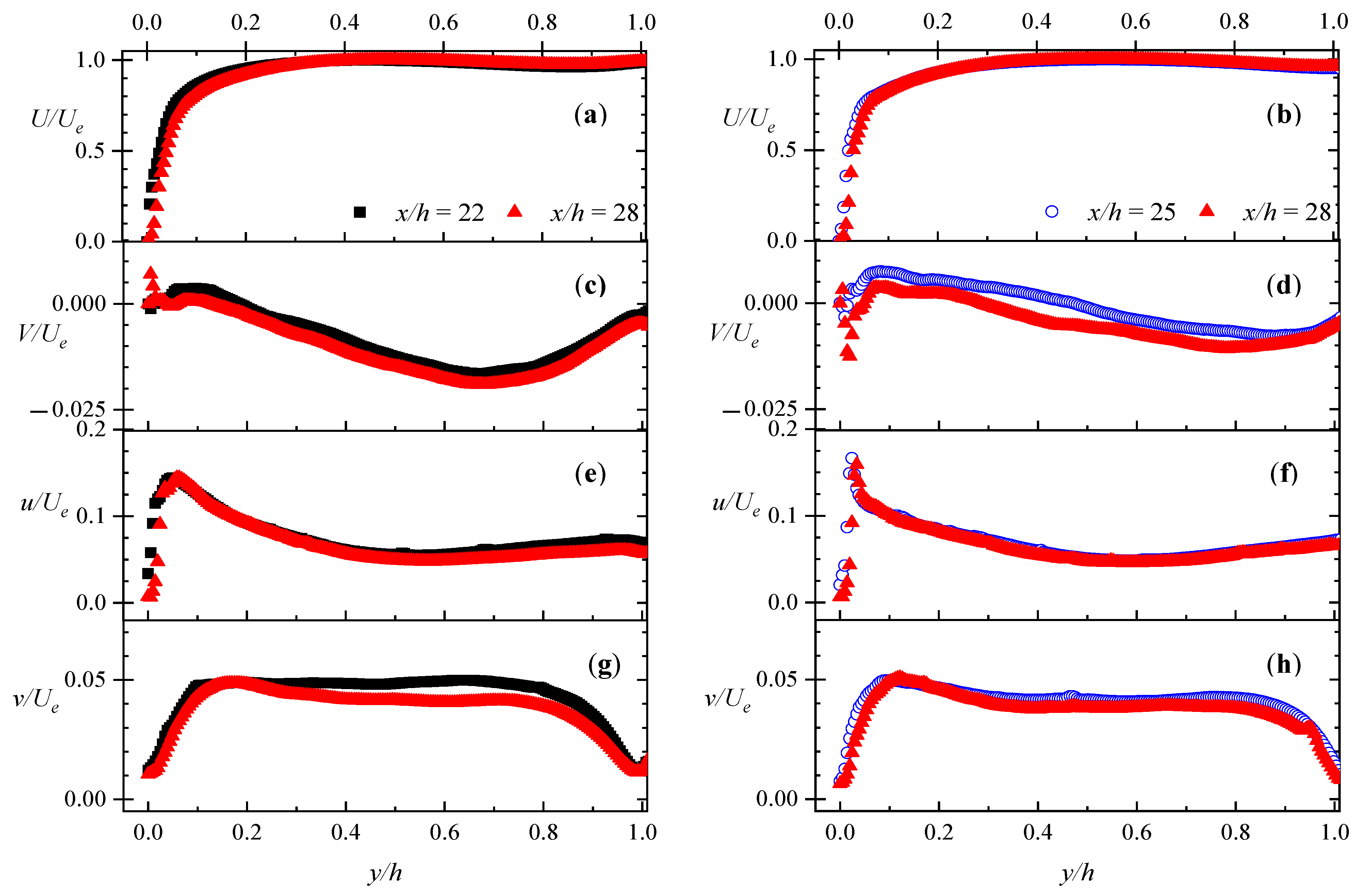
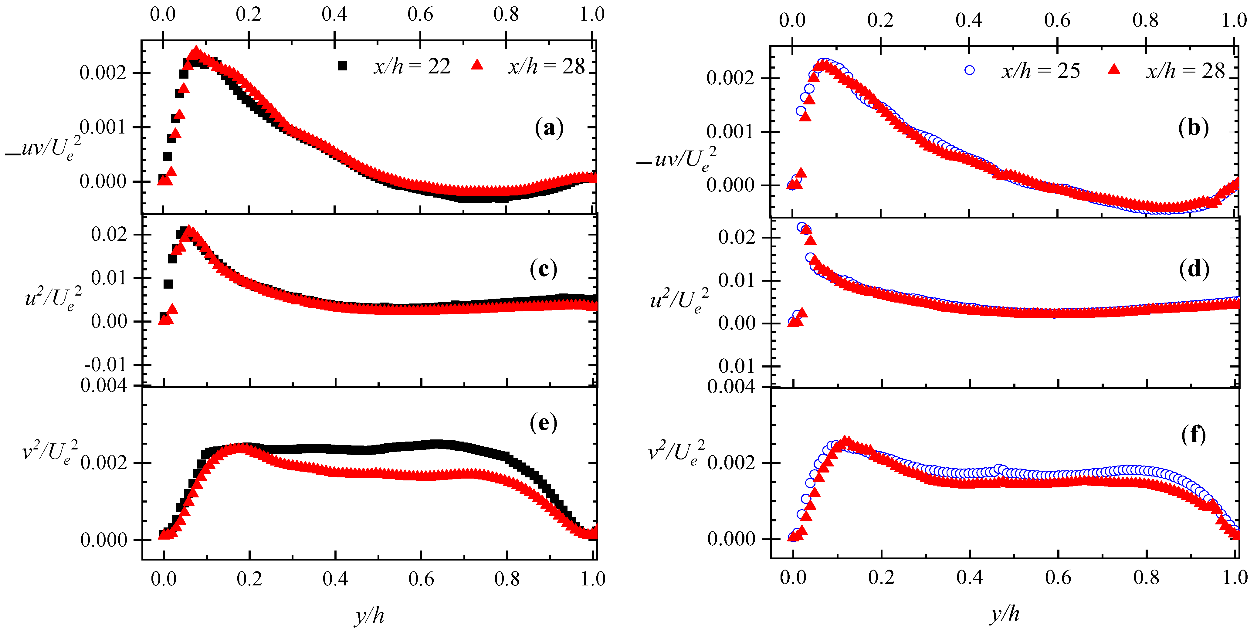
In order to show the nature of flow development for the present tests, a wide range of the flow data are extracted from representative measurements taken during test conditions AR1.5Re165Fr0.13 and AR1.3Re452Fr0.17. According to Kirkgöz and Ardiclioglu [7], the expected flow developing zone for the range of flow conditions covered herein should be between 51 h and 60 h. However, the current data were taken much further upstream (16 < x/h < 29). Thus, the following section presents unique and detailed insight into the nature of the flow development (if any) of a narrow open-channel flow prior to the developing zone. The results of the mean velocities and turbulent statistics normalized by the local maximum velocity are plotted in Figure 2 and Figure 3. They show that while the streamwise components of the mean velocities and turbulent intensities appear to be independent of the streamwise location, the wall-normal components are not. Additionally, the wall-normal Reynolds stress profiles at increasing streamwise locations do not converge. While the spanwise components were not measured (due to the limitations of the PIV arrangement), it is reasonable to expect that at the locations of measurement, those velocities would likely be dependent on the streamwise location as well. Consequently, Figure 2 and Figure 3 confirm that the flow is not fully developed [10].
Apart from this foregoing conclusion, it is important to note some particular traits. The results indicate that at a higher Reynold’s number, the deviation of the wall-normal mean velocities from full development is much more apparent. In contrast, the wall-normal turbulent intensities tend toward streamwise independence as Reynolds number increases. While subject to confirmation, it is reasonable to speculate that the lack of flow development in the wall-normal mean and turbulence quantities may be the result of strong three-dimensional effects. This is very likely due to the extreme narrowness of the channel. The wall-normal intensities, on the other hand, may not be affected by such wall-effects.
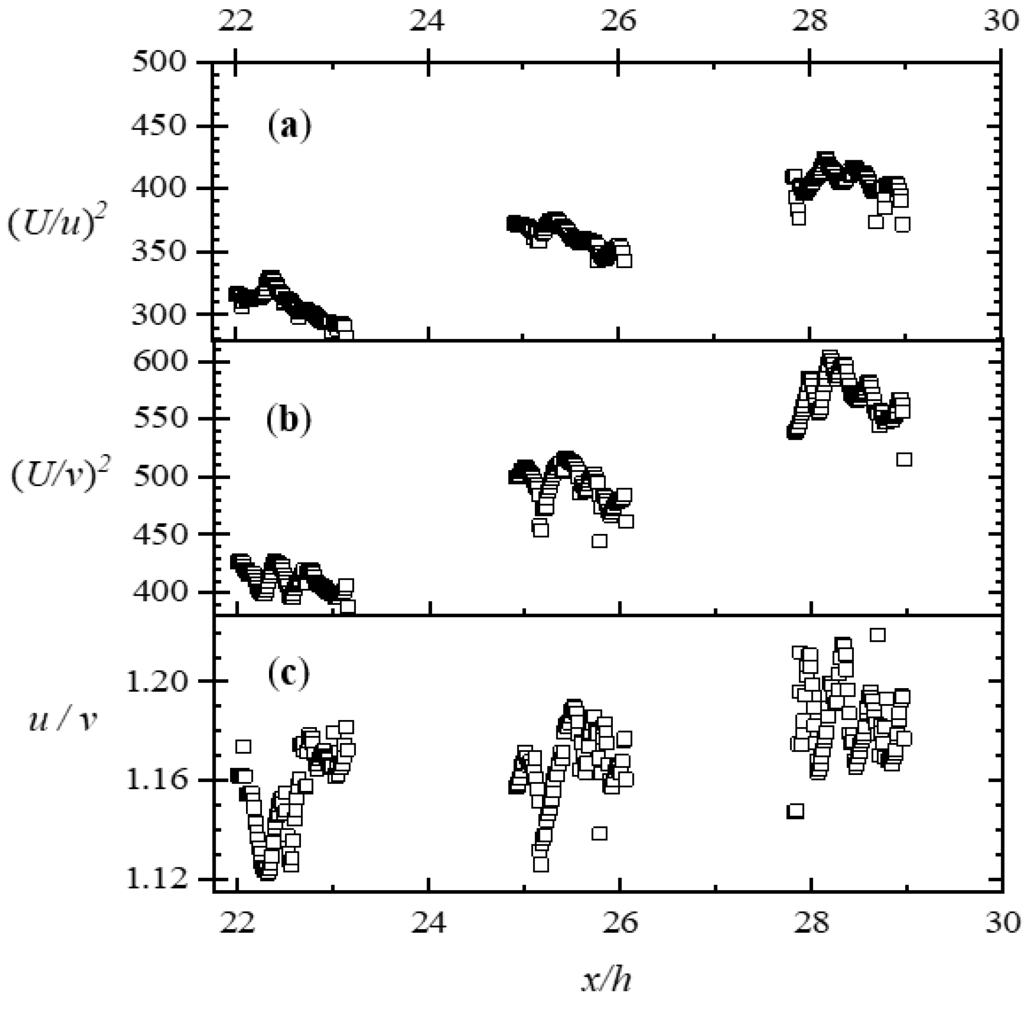
In Figure 4, the levels of turbulence decay and turbulence anisotropy during the development of the flow are presented. This is achieved using data extracted from the mid-depth of the flow (i.e., y = h/2). The profiles of turbulence decay in the streamwise direction (U/u)2 and that in the wall-normal directions (U/v)2 show that the latter is significantly higher than the former. These indicate that streamwise development of flow tends to dampen the large scales of the flow. It is important to point out that the current values of these turbulence intensity ratios are at least two times those reported by Mahananda et al. [10]. This may be attributed to the presence of bed roughness in the latter work, which could inhibit the decay of turbulence in a developing flow.
An examination of the turbulence flow mid-depth anisotropies (u/v) in Figure 4 also shows that the streamwise turbulence intensities are 12–22% larger than the wall-normal components. The global and local variations relative to the streamwise direction are significant, with the latter trending in the direction of an increasing anisotropy along the stream. These observations are important as they signify an evolving process of energy transfer to the streamwise turbulence intensities due to the energy cascade. Again, comparing this work with Mahananda et al. [10], it is clear that the addition of roughness elements can lead to an enhancement of the anisotropy levels of a developing flow in a narrow channel by over 50%.
3.2. Characteristics of the Mean Flow
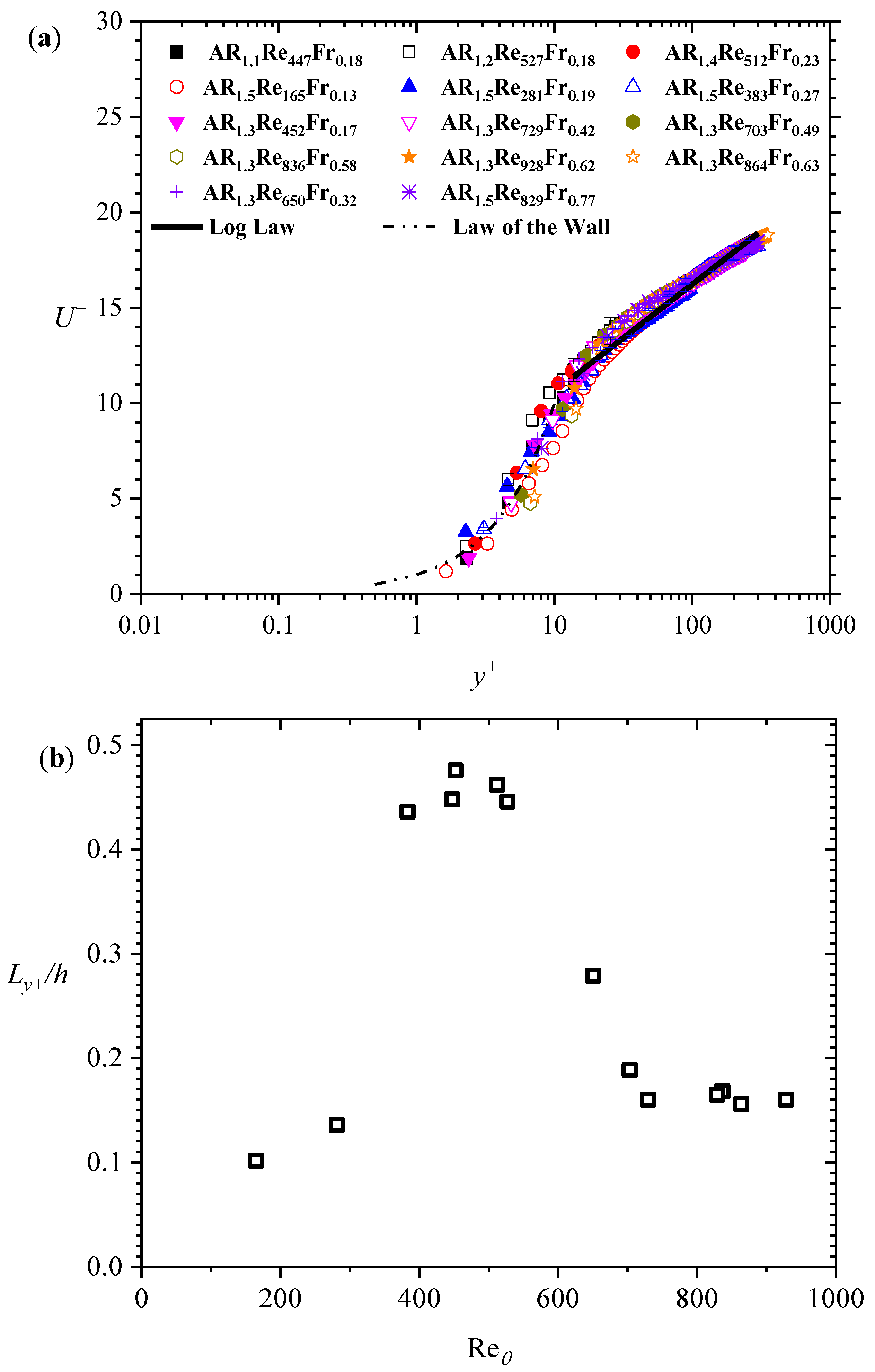
In characterizing the flow, attention is first turned to the results of the mean flow presented in Figure 5, Figure 6, Figure 7 and Figure 8 and Table 2. The developing boundary layer of the narrow channel studied in this work has certain features similar to those of other open-channel flows. This is already demonstrated in Figure 2. Consequently, the flow may be properly stratified into the conventional inner and outer regions, and analyzed as such. Plots of the streamwise mean velocity in inner wall units (i.e., U+ = U/ Uτ and y+ = y Uτ /ν, for a characteristic friction velocity Uτ) in Figure 5, show the presence of a portion of a viscous sublayer that appears to conform to the following well-known law of the wall:
This law is accepted to be valid up to y+ 5 in other turbulent boundary layer flows. Beyond y+ 5, however, a logarithmic layer exists. Like other turbulent boundary layers, each test condition in this work is found to have a logarithmic layer following the classical logarithmic (log) law, namely:
A von Kármán constant κ ranging from 0.40 to 0.41, and a logarithmic law constant B from 5.0 to 6.0 both satisfy this law for the current test data. The consistency is so remarkable that when using these constants in a Clauser plot technique, the optimal values of Uτ may be obtained within a maximum relative deviation of 3.5%. For brevity, however, only the friction parameters obtained from Equation (2) with constants κ = 0.41 and B = 5.0 are presented in Table 2 and analyzed hereafter. In general, the logarithmic layer is found to fall within a wall-normal range (Ly+) of 30 < y+ 300. For the tests with the lowest Reynolds number (i.e., AR1.5Re165Fr0.13 and AR1.5Re281Fr0.19), the upper limit of this layer is much less than y+ = 300, but such that y 0.2 h. The logarithmic layer tends to diminish (<15% of the flow depth) with a decreasing Reynolds number. However, as shown in Figure 5, this is not a monotonic trend. The current tests indicate that irrespective of AR, the thickness of the layer for a low Reynolds number flow peaks to over 45% of the flow depth, at around 350 < < 550, which is then followed by a decline and a levelling off with an increasing Reynolds number.
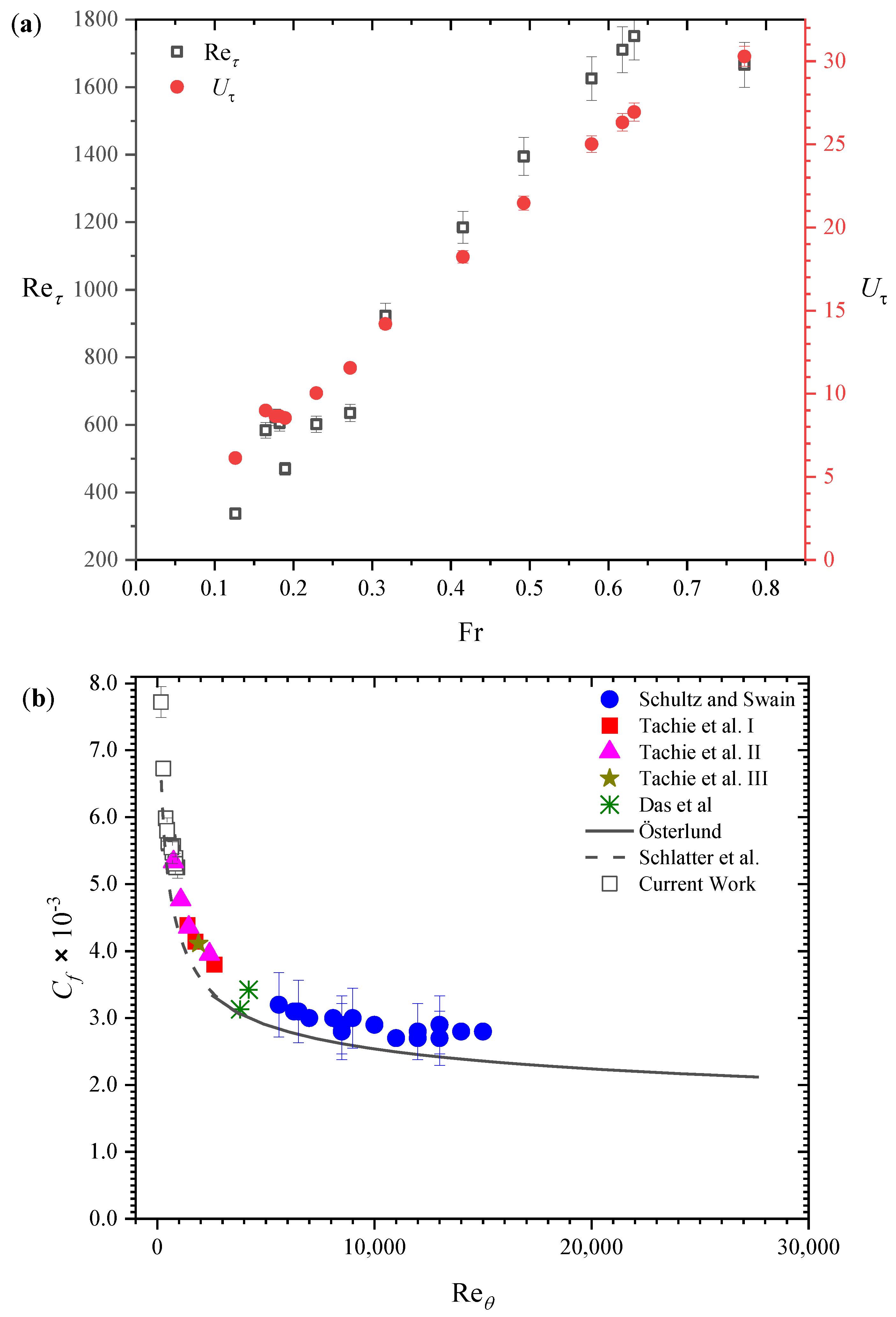
The log-linear plots in Figure 5 clearly show that like other boundary layer flows, Uτ is an important wall parameter with dominant effects close to the bed of the channel. Nevertheless, it must be emphasized that Uτ is not only dependent on the local conditions. On the contrary, there is evidence of a direct dependence of the outer layer effects of the flow surface, such that Uτ may be predicted by the Froude number Fr. Consequently, a friction Reynolds number defined by the friction velocity Uτ and the flow depth h, exhibits a strong dependency on Fr. The current data plotted in Figure 6 show that the relationships are linear, and defined by the following:
and
with adjusted R2 values of 0.997 and 0.985, respectively.
Another friction parameter considered in this work is the skin friction coefficient Cf. This is computed from the mean velocity data as two (Uτ/Ue)2. In order to provide a comparison of the friction parameters with those reported in other works, the skin friction coefficient is plotted in Figure 6 along with those published in several other open-channel flow studies. The data compared are derived from Uτ measurements in the mid-span plane. As depicted in the figure, the variation of Cf. with trends is similar to other works, irrespective of the differences in the aspect ratio of those works. Thus, mid-span values of Cf are not affected by the aspect ratio of the channel. Indeed, like other turbulent boundary layer flows, this coefficient tends to increase logarithmically with decreasing . However, in the case of open-channel flows, this coefficient may be predicted up to of about 15,000 through the following equation:
The adjusted R2 for such a fit is 0.979. In 1999, Tachie et al. [14] noted subtle differences between Cf obtained from open-channel flows and others, such as wind tunnel measurements, or simulations of classical turbulent boundary layer flows. With a wider range of published data (such as that provided in this work), more precise confirmations of the differences may be made. When compared with other turbulent boundary layer fits, such as that prescribed by Österlund [15] and Schlatter et al. [16], the Cf values from Equation (5) converge as decreases and appear to diverge beyond 1000. While this observation requires further investigation, it is reasonable to infer that such a difference is likely associated with the non-local (outer layer) free surface effects on the friction.
Figure 6.
(a) Dependence of friction velocity Uτ and friction Reynolds number on the Froude number Fr. (b) Skin friction coefficient Cf values of current tests compared with other open-channel flow studies (Schultz and Swain [17]; Tachie et al. I [4], II [6], III [18] and; Das et al. [19]) and other boundary layer studies (Österlund [15] and Schlatter et al. [16]).

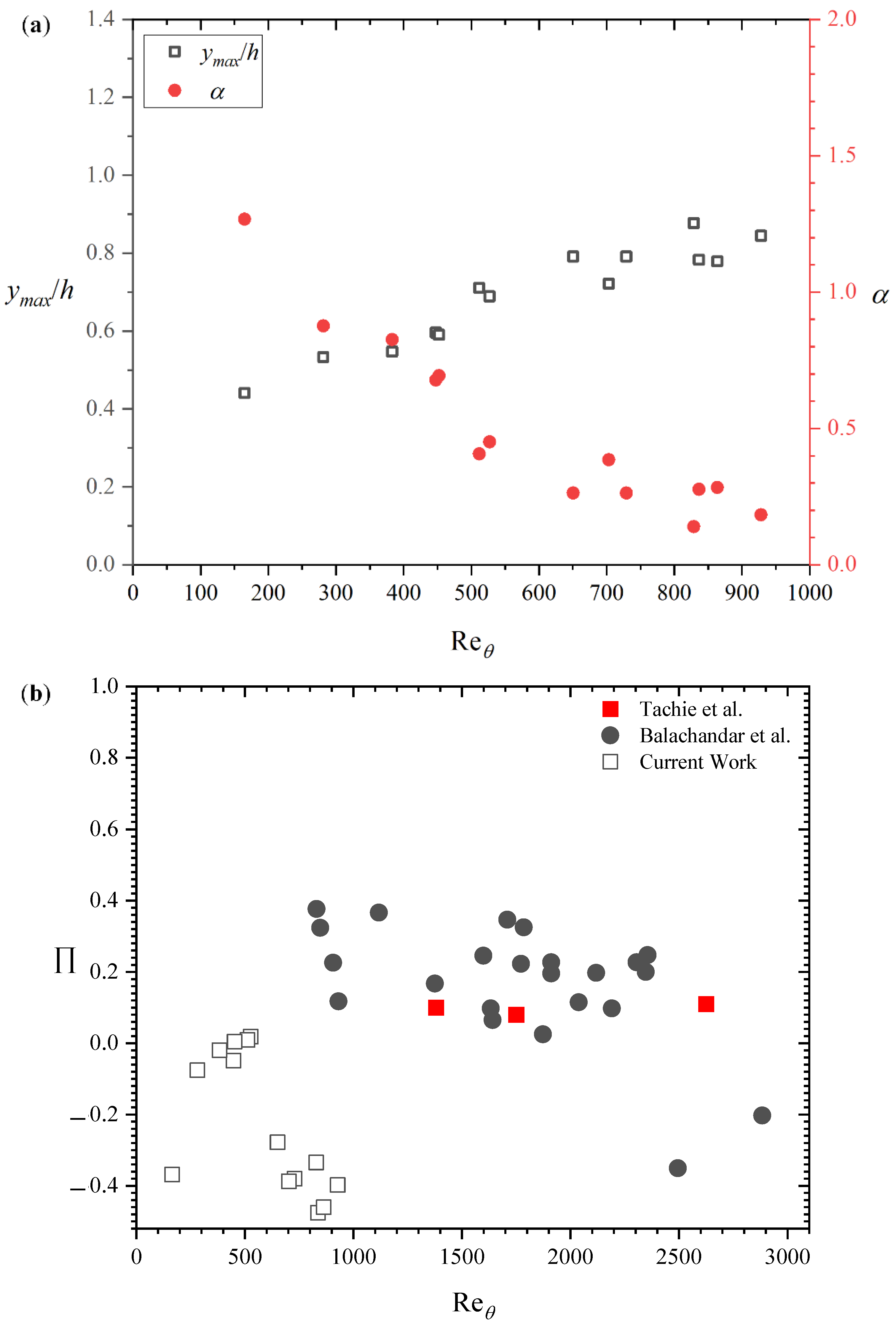
For the outer flow, some of the most consequential parameters are the maximum streamwise mean velocity Ue, the wall-normal location of that maximum velocity ymax, and the flow depth h. The occurrence of the maximum velocity below the flow depth (i.e., dip phenomenon) is characteristic of narrow open-channel flows. This phenomenon is shown in Figure 7 in terms of ymax/h and a dip correction factor . The data show that both parameters are functions of the Reynolds number . This is an important finding, as previous works have only noted that the dip correction factor is mainly affected by the spanwise location of the measurement, and hitherto the other affecting factors have not been explored. However, with the data presented herein, we can now see that for ymax/h or , the relationship with is significant, linear, and even predictable over the narrow range of Reynolds number studied in this work through the following equation:
The adjusted R2 for such a fit is 0.857. Furthermore, the trend (see Table 2, Figure 7) indicates that regardless of the ultra-narrowness of the channel, the dipping phenomenon is expected to reduce with increasing . The scatter in the data at high Reynolds number is patent. However, this may be the result of discernible effects of medium Fr number.
The deviation of the outer flow from the log law is often characterized by the wake parameter ∏. Some researchers [20] have incorporated such a parameter in a streamwise mean velocity defect profile given by the following:
Using Equation (7) and the Uτ already evaluated, ∏ values may be obtained for each test condition within 0.1 ≤ y/δ ≤ 1. The results are summarized in Table 2 and plotted in Figure 7. In that figure, the results are compared with two other measurements that are associated with open-channel turbulent flows over smooth walls. It is noted that for both test data taken from references [4] and [21], the data are in the range 830 < Reθ < 3000. Of the two data sets, the results from reference [21] have the largest recorded Fr of up to unity. The ∏ values reported herein are much lower than the 0.55 value quoted for zero pressure gradient smooth plate flow. Additionally, there is no clear trend of dependency with Reθ or Fr. One implication of these observations is that the free surface effects infiltrate deep into all regions of the boundary layer [21], dampening the inner and outer layer disparities.
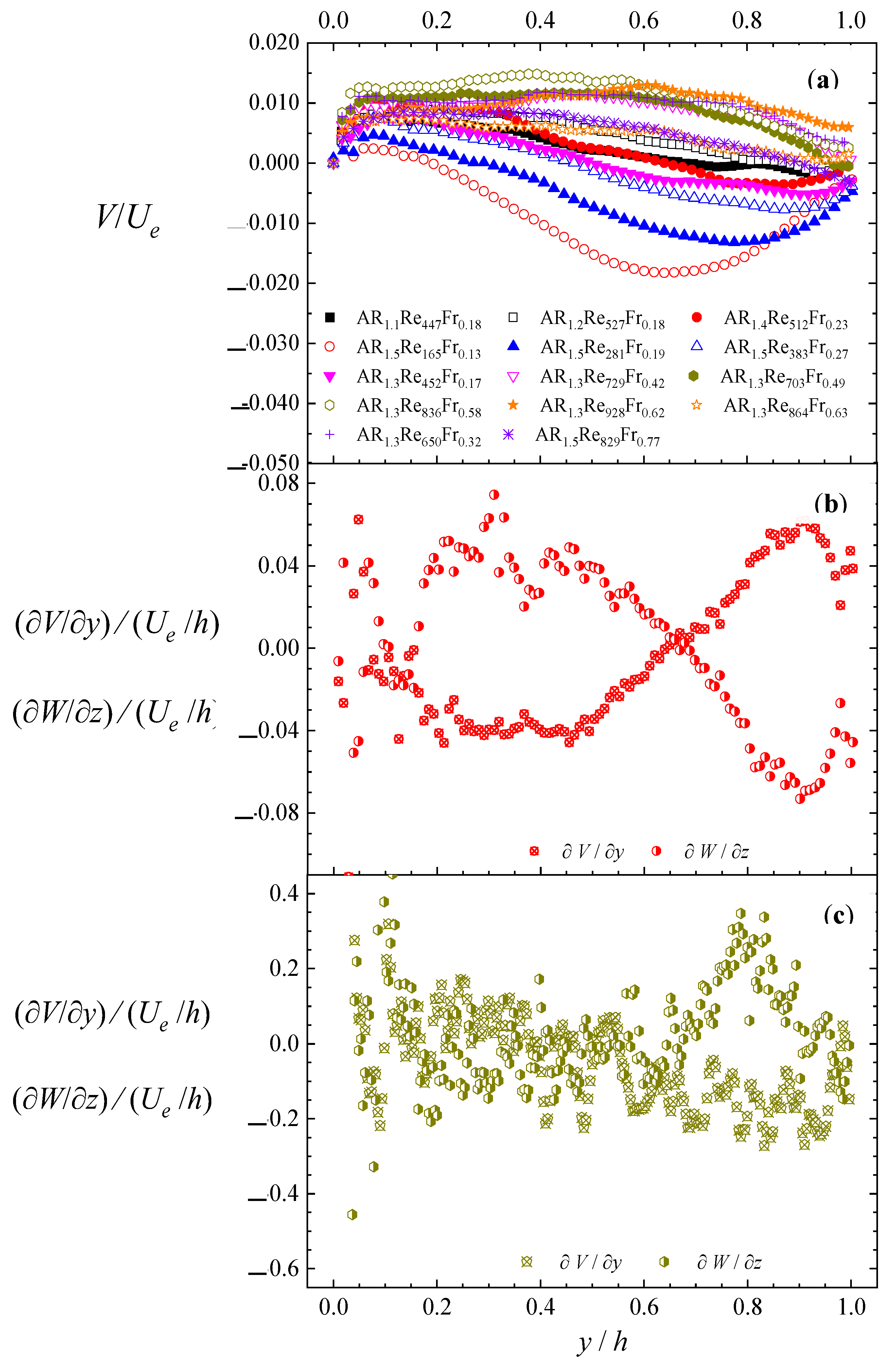
An examination of the wall-normal velocities and gradients of the wall-normal and spanwise velocities in Figure 8 provides some insight into the nature of the dipping phenomenon. The dip observed in the mean streamwise velocity distribution is often attributed to large-scale secondary flow patterns from the corner toward the mid-span of the channel. The observations of this work seem to point to a culmination of multi-dimensional motion around the mid-depth region of the mid-span plane. Consequently, a significant downward movement (V < 0) of flow toward the bed is recorded at that location. The values increase with the Reynolds number. The wall-normal gradients in the streamwise wall-normal velocity (∂V/∂y) and the spanwise gradients in the mean spanwise flow (∂W/∂z, assessed from the continuity equation) are comparable. At the highest Reynolds numbers tested in this work, the trend in the distribution of the velocity gradients are unclear. However, at low Reynolds numbers, ∂V/∂y and ∂W/∂z are at least five times that of the streamwise gradient of the mean streamwise velocity (∂U/∂x). The significant values of ∂W/∂z indicate there may be a movement of flow directed from the sidewalls toward the mid-span plane, and changes in flow directions. The dynamic changes in ∂V/∂y and ∂W/∂z, being more prevalent at around y/h > 0.5, suggest that they may be significant contributors to the dipping phenomenon observed below the surface of the flow.
Figure 7.
(a) Dependence of the location of the maximum streamwise mean velocity ymax on , shown in dimensionless parameters (ymax/h and a dip correction factor ). (b) Cole’s wake parameter for current test data compared with other open-channel flow studies (Tachie et al. I [4] and Balachandar et al. [21]).

Figure 8.
(a) Dependence of the normalized mean wall-normal velocities (V/Ue) on the wall-normal location. Gradients of the streamwise wall-normal and spanwise velocities (∂V/∂y and ∂W/∂z) for (b) AR1.5Re165Fr0.13 and (c) AR1.3Re836Fr0.58.
Figure 8.
(a) Dependence of the normalized mean wall-normal velocities (V/Ue) on the wall-normal location. Gradients of the streamwise wall-normal and spanwise velocities (∂V/∂y and ∂W/∂z) for (b) AR1.5Re165Fr0.13 and (c) AR1.3Re836Fr0.58.

3.3. Characteristics of Higher-Order Moments of the Turbulence Statistics
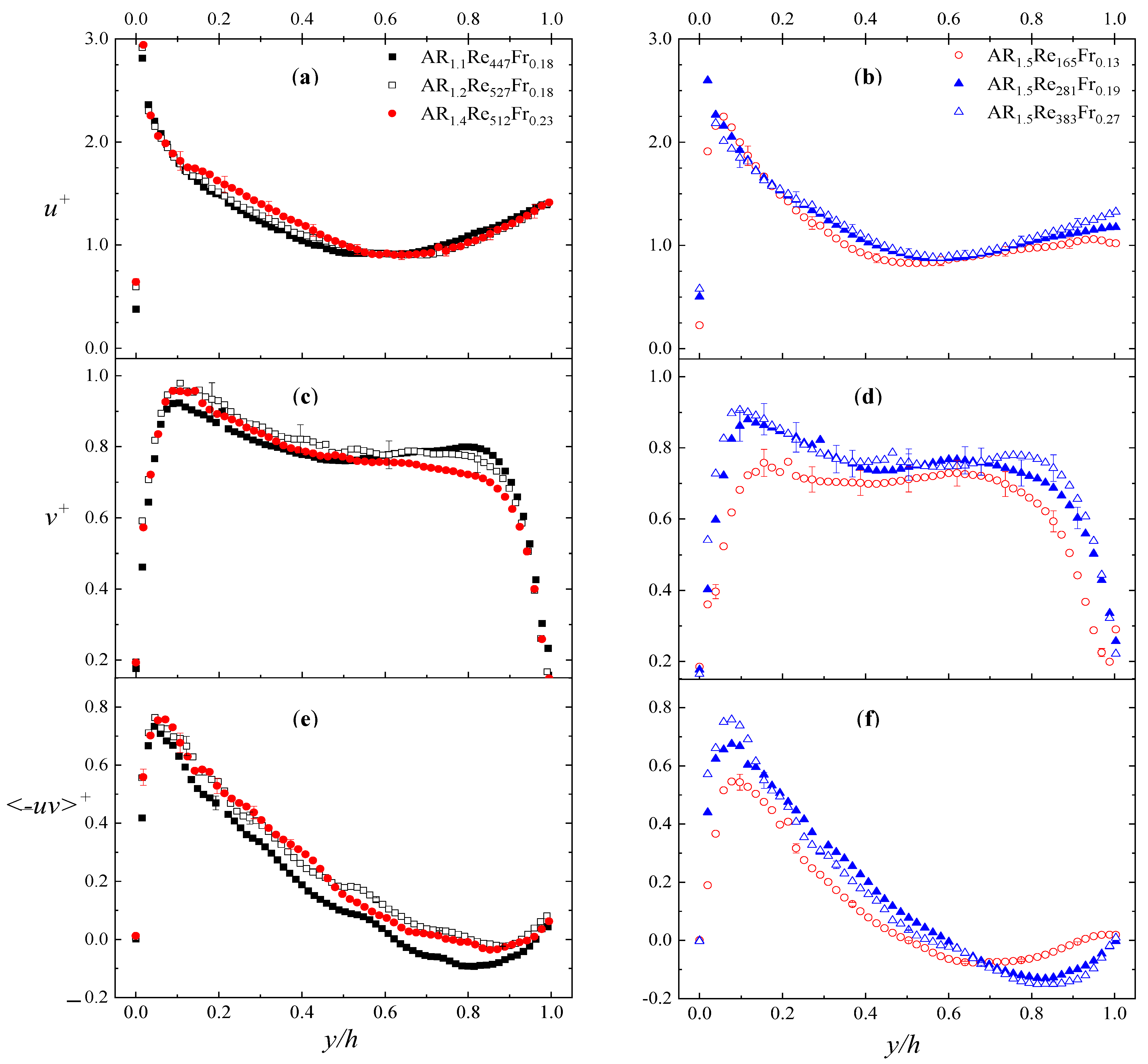
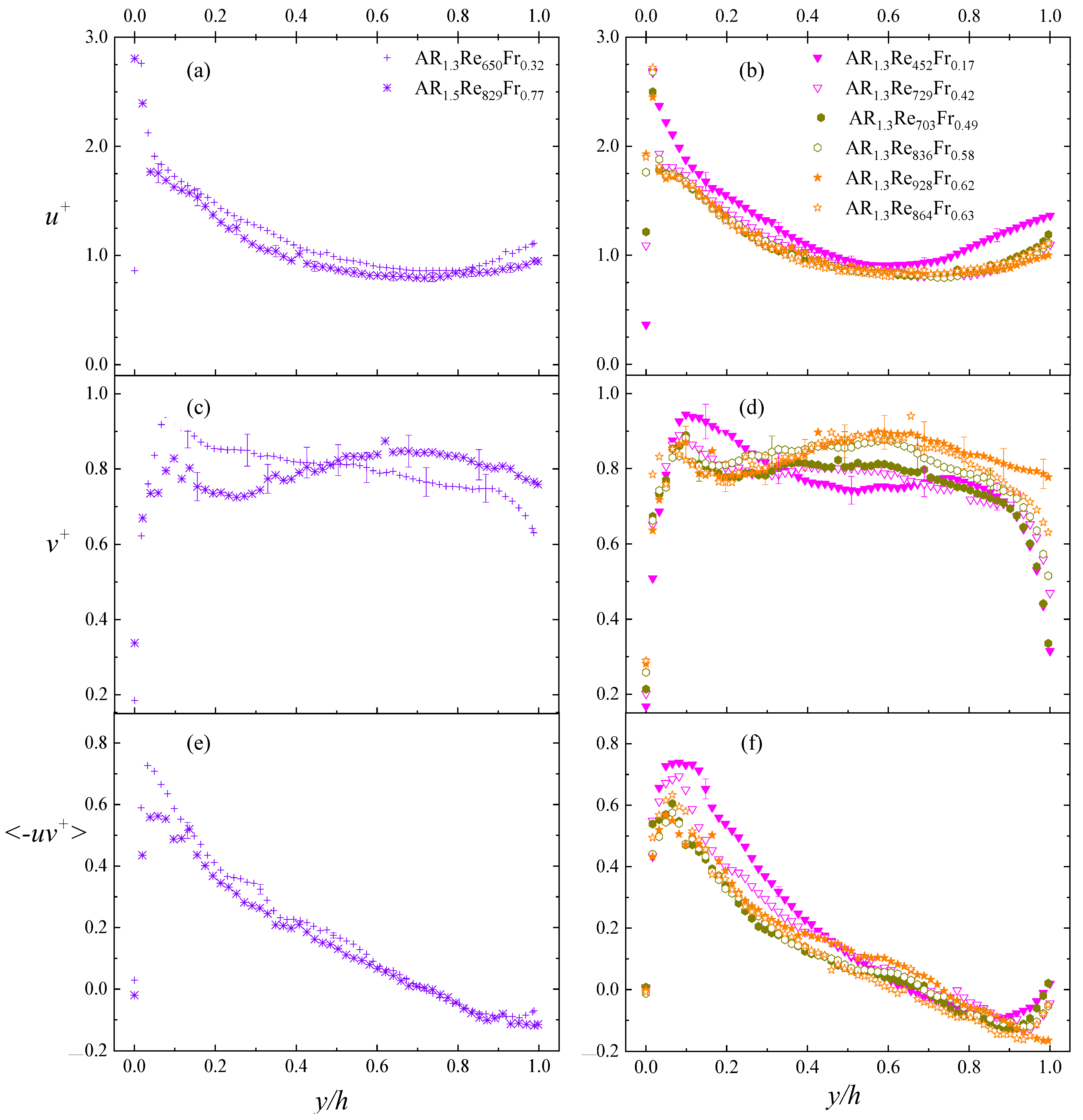
The higher-order moments of turbulence statistics are considered by focusing on the turbulence intensities and Reynolds shear stresses. The Reynolds normal stresses are omitted because they are qualitatively similar to the corresponding turbulent intensities. The turbulence intensity and Reynolds shear stress data are normalized by the friction velocities, plotted against the wall-normal coordinate per flow depth, and presented in Figure 9 and Figure 10. In order to allow for the systematic study of the parametric effects, the plots are shown to determine any trend due to comparatively large AR changes (Figure 9a,c,e), changes (Figure 9b,d,f), Fr changes (Figure 10a,c,e), and combined AR and modifications (Figure 10b,d,f).
Attention is first focused on the turbulence intensity profiles. These represent the level of velocity fluctuations in the flow. It is important to point out that for the entire depth of the flow, the normalized streamwise turbulence intensities (u+) are significantly larger than the wall-normal components (v+). While the difference in the turbulence intensities peaks at regions close to the wall, it reduces toward the mid-depth region. This is consistent with the observations noted in an earlier section regarding enhanced wall-normal flow motion around the mid-depth region. Another point to note about the turbulence intensity plots is that while the directions of the trends of u+ and v+ are generally similar, they move in opposite directions as the free surface is approached. The increasing values of u+ close to the free surface indicate that the surface effects are much more dominant in the flow direction, thus enhancing fluctuations in that direction, and attenuating those in the wall-normal direction. Compared with data from previous studies of open-channel turbulent flows, the turbulence intensities reported here are significantly different. This is expected due to differences in the streamwise location of measurements. Thus, while the peak value of u+ in Figure 9 is, for instance, ~10% greater than that reported by Tachie et al. [18], the former is expected to decay at a location of fully developed flow.
Again, with respect to the turbulence intensities, it is noteworthy that in the region 0.1 < y/h < 0.9, v+ values do not show any significant variations with AR and when both parameters are low (i.e., AR < 1.5; < 400). However, a substantial increase in Fr (for instance, from 0.32 to 0.64) leads to clear reductions in turbulent intensities at 0.2 < y/h < 0.4 and 0.9 < y/h < 1.0. Additionally, the combined effect of modifying and Fr (in particular, increasing Fr by over 3 times at > 400) results in marked reductions in streamwise turbulent intensities, outside of the experimental error or scatter. The plots in Figure 10 show that those deviations are centered around the regions close to the bed and the free surface. The pervasiveness of these effects raises doubts as to the existence of a universal function for streamwise turbulence intensities in open-channel flows. Specifically, the current data suggest that the universal functions for streamwise and wall-normal turbulence intensities proposed by Nezu and Rodi [22] will not apply to developing narrow open-channel low Reynolds number flows. This is a significant observation, given that those functions were proposed by these researchers as the basis of a simplified k-ɛ turbulence model.
The Reynolds shear stresses denote the momentum fluxes of the unsteady turbulent motions that work effectively as additional shear stresses. Unlike two-dimensional flows, the wall-normal distributions of these stresses (<uv>+) shown in Figure 9 and Figure 10 are from a three-dimensional flow. Consequently, they are characterized by maximum and minimum points and changes in sign value. The latter characteristic is particularly consistent with the velocity dipping phenomenon. It is important to note that the plots show that the <uv>+ profiles are affected by AR, , and Fr. Such effects are associated with various sections of the flow depth. By increasing the AR from 1.1 to 1.4, the effective shear stresses due to turbulent fluctuations increase by up to 450% over the range 0.2 < y/h < 0.9. Any increment in the flow factors allied with a substantial change in Fr, on the other hand, tends to decrease those stresses within a more restricted depth range (0 < y/h < 0.4). Perhaps the most effective changes in Reynolds shear stress are obtained by varying the Reynolds number. Increasing leads to an increment in <uv>+ at 0 < y/h < 0.7, and a decrement at y/h > 0.7. The location of the maximum value of <uv>+ appears not to follow any particular trend with respect to . However, the minimum value of <uv>+ varies nearly linearly from y/h = 0.65 to 0.99 as increases from 165 to 928. Overall, the complexity of the profiles cautions a re-assessment of the simplified momentum relations of the Reynolds equation used in the evaluation of the friction velocity.
To provide an additional comparison of the present flow with other canonical flows, the relative effects of the turbulence intensities and the Reynolds shear stress may be assessed through the correlation coefficient (i.e., the ratio of the Reynolds shear stress and the product of u and v). The outcome is a range of values from 0.1 to 0.5 within 0.1 ≤ y/h ≤ 0.6. This result is in contrast with other open-channel and boundary layer flows where such a section is reported to yield a nearly constant correlation coefficient value of 0.4–0.5 [1]. This further demonstrates the significant differences in the variation of turbulence intensities and Reynolds numbers, compared with other turbulent boundary layers.
4. Summary and Conclusions
Particle image velocimetry has been used to obtain velocity measurements of an open-channel flow in the developing section of a flume with a narrow width. The aspect ratio (AR) of the flow was varied from 1.1 to 1.5 using a variant depth of flow h. The Reynolds numbers based on the momentum thickness and Froude number Fr were also in the ranges of ~160 to 930 and 0.1 to 0.8, respectively.
This work demonstrates that the developing turbulent flow zone may be encountered at a much further upstream location (16 < x/h < 29) for a tripped flow. Yet, for such a flow, only the streamwise components of the velocities are independent of the streamwise location. For a developing open-channel turbulent flow over a smooth wall, the mean flow consists of an inner and outer flow structure. For the inner layer, there exists a logarithmic layer following the classical log law with a von Kármán constant ranging from 0.40 to 0.41, and a log law constant of 5.0 to 6.0. The friction velocity obtained through the Clauser plot technique may also be predicted through a linear equation associated with Fr. Utilizing the current data and other data in the literature, a new logarithmic equation has been proposed to predict the skin friction coefficient Cf with the knowledge of alone. For the outer flow, it is shown that the wall-normal location of the maximum velocity ymax/h occurs below the flow depth. Its associated dip correction factor is a predictable linear function of . The wake parameter is also found to range from −0.50 to 0.02, irrespective of the Reθ, Fr, or AR. With respect to the higher-order turbulence statistics, the turbulence intensities indicate values that are consistent with an enhanced wall-normal flow motion around the mid-depth region. The wall-normal distributions of the Reynolds shear stresses also reveal distinctive minima, along with sign changes, due to dipping. There is a clear deviation of the correlation coefficient (ranging from −0.1 to 0.5) from other open-channel flows.
An important conclusion derived from this work is that while some of the dynamics of the unconstrained open-channel flow studied herein may be predicted using mean flow assessment tools applied to conventional open-channel flows, there are important differences. The implication of the foregoing on the evaluation of friction parameters and turbulence modeling assessments is potentially significant and requires further probing.
Funding
This work was not funded by any external grant.
Data Availability Statement
Not applicable.
Acknowledgments
The support of this work through the C. Graydon and Mary E. Rogers Fellowship is gratefully acknowledged.
Conflicts of Interest
The author declares no conflict of interest.
Nomenclature
| English | |
| B | logarithmic law constant |
| b | width of test channel |
| Cf | skin friction coefficient =2 (Uτ/Ue)2 |
| g | acceleration due to gravity |
| h | depth of flow |
| H | depth of test channel |
| L | length of test channel |
| Ly+ | range of log layer in inner coordinates |
| Reθ | Reynolds number based on maximum velocity and momentum thickness |
| Reh | Reynolds numbers based on the maximum streamwise mean velocity and flow depth |
| Reτ | Reynolds numbers based on the friction velocity and flow depth |
| U | mean (time-averaged) streamwise velocity |
| u | streamwise turbulence intensity |
| u+ | streamwise turbulence intensity in inner coordinates = u/Uτ |
| u2 | streamwise Reynolds normal stress |
| Ub | depth-averaged mean streamwise velocity |
| Ue | maximum mean streamwise velocity |
| Uτ | friction velocity |
| U+ | time-averaged streamwise velocity in inner coordinates = U/Uτ |
| uv | Reynolds shear stress |
| <uv>+ | Reynolds shear stress in inner coordinates = uv/Uτ2 |
| V | mean (time-averaged) wall-normal velocity |
| v | wall-normal turbulence intensity |
| v+ | streamwise turbulence intensity in inner coordinates = v/Uτ |
| v2 | wall-normal Reynolds normal stress |
| W | mean (time-averaged) spanwise velocity |
| x | streamwise direction; streamwise distance |
| y | wall-normal direction; wall-normal distance |
| y+ | wall-normal direction in inner coordinates = y Uτ /ν |
| ymax | location of the mean streamwise velocity |
| z | spanwise direction; spanwise distance |
| Greek | |
| dip correction factor | |
| δ | boundary layer thickness |
| δ * | displacement thickness |
| θ | momentum thickness |
| von Kármán constant | |
| ν | kinematic viscosity |
| ∏ | Cole’s wake parameter |
| Other Symbols/Acronyms | |
| ADV | acoustic Doppler velocimetry |
| AR | aspect ratio (b/h) |
| Fr | Froude number |
| ℌ | boundary layer shape parameter, =δ */θ |
| LDA | laser Doppler anemometry |
| PIV | particle image velocimetry |
| PVC | polyvinyl chloride |
References
- Nezu, I. Open-Channel Flow Turbulence and Its Research Prospect in the 21st Century. J. Hydraul. Eng. 2005, 131, 229–246. [Google Scholar] [CrossRef]
- Sarma, K.V.N.; Lakshminarayana, P.; Rao, N.S.L. Velocity Distribution in Smooth Rectangular Open Channels. J. Hydraul. Eng. 1983, 109, 270–289. [Google Scholar] [CrossRef]
- Balachandar, R.; Ramachandran, S.S. Turbulent Boundary Layers in Low Reynolds Number Shallow Open Channel Flows. J. Fluids Eng. 1999, 121, 684–689. [Google Scholar] [CrossRef]
- Tachie, M.F.; Bergstrom, D.J.; Balachandar, R. Rough Wall Turbulent Boundary Layers in Shallow Open Channel Flow. J. Fluids Eng. 2000, 122, 533–541. [Google Scholar] [CrossRef]
- Bergstrom, D.J.; Tachie, M.F.; Balachandar, R. Application of power laws to low Reynolds number boundary layers on smooth and rough surfaces. Phys. Fluids 2001, 13, 3277–3284. [Google Scholar] [CrossRef]
- Tachie, M.F.; Balachandar, R.; Bergstrom, D.J. Low Reynolds number effects in open-channel turbulent boundary layers. Exp. Fluids 2003, 34, 616–624. [Google Scholar] [CrossRef]
- Kirkgöz, M.S.; Ardiçlioğlu, M. Velocity Profiles of Developing and Developed Open Channel Flow. J. Hydraul. Eng. 1997, 123, 1099–1105. [Google Scholar] [CrossRef]
- Sarkar, S. Measurement of turbulent flow in a narrow open channel. J. Hydrol. Hydromech. 2016, 64, 273–280. [Google Scholar] [CrossRef]
- Mahananda, M.; Hanmaiahgari, P.; Balachandar, R. Effect of aspect ratio on developing and developed narrow open channel flow with rough bed. Can. J. Civ. Eng. 2018, 45, 780–794. [Google Scholar] [CrossRef]
- Mahananda, M.; Hanmaiahgari, P.; Balachandar, R. On the turbulence characteristics in developed and developing rough narrow open-channel flow. J. Hydro-Environ. Res. 2022, 40, 17–27. [Google Scholar] [CrossRef]
- Arthur, J.K. Turbulent Flow through and over a Compact Three-Dimensional Model Porous Medium: An Experimental Study. Fluids 2021, 6, 337. [Google Scholar] [CrossRef]
- Arthur, J.K. A narrow-channeled backward-facing step flow with or without a pin–fin insert: Flow in the separated region. Exp. Therm. Fluid Sci. 2023, 141, 110791. [Google Scholar] [CrossRef]
- Wieneke, B. PIV uncertainty quantification from correlation statistics. Meas. Sci. Technol. 2015, 26, 074002. [Google Scholar] [CrossRef]
- Tachie, M.F.; Bergstrom, D.J.; Balachandar, R.; Ramachandran, S. Skin Friction Correlation in Open Channel Boundary Layers. J. Fluids Eng. 2001, 123, 953–956. [Google Scholar] [CrossRef]
- Österlund, J.M. Experimental Studies of Zero Pressure-Gradient Turbulent Boundary Layer Flow. Ph.D. Thesis, Royal Institute of Technology, Stockholm, Sweden, 1999. [Google Scholar]
- Schlatter, P.; Li, Q.; Brethouwer, G.; Johansson, A.V.; Henningson, D.S. Structure of a turbulent boundary layer studied by DNS. In Direct and Large-Eddy Simulation VIII; Springer: New York, NY, USA, 2011. [Google Scholar]
- Schultz, M.P.; Swain, G.W. The Effect of Biofilms on Turbulent Boundary Layers. J. Fluids Eng. 1999, 121, 44–51. [Google Scholar] [CrossRef]
- Tachie, M.F.; Bergstrom, D.J.; Balachandar, R. Roughness effects in low-Re θ open-channel turbulent boundary layers. Exp. Fluids 2003, 35, 338–346. [Google Scholar] [CrossRef]
- Das, S.; Balachandar, R.; Barron, R. Generation and characterization of fully developed state in open channel flow. J. Fluid Mech. 2022, 934, A35. [Google Scholar] [CrossRef]
- Krogstad, P.; Antonia, R.A.; Browne, L.W.B. Comparison between rough- and smooth-wall turbulent boundary layers. J. Fluid Mech. 1992, 245, 599–617. [Google Scholar] [CrossRef]
- Balachandar, R.; Blakely, D.; Tachie, M.F.; Putz, G. A Study on Turbulent Boundary Layers on a Smooth Flat Plate in an Open Channel. J. Fluids Eng. 2001, 123, 394–400. [Google Scholar] [CrossRef]
- Nezu, I.; Rodi, W. Open-channel Flow Measurements with a Laser Doppler Anemometer. J. Hydraul. Eng. 1986, 112, 335–355. [Google Scholar] [CrossRef]
Figure 1.
(a) Experimental set-up, and (b) schema of the test section and the coordinate system employed in this work. The green shaded section in (b) covers the focus of PIV measurement. All dimensions are in millimeters. The symbols x, y, and z represent the directions along the stream, wall-normal, and the span, respectively.

Figure 2.
Wall-normal variations of streamwise mean velocities (a,b), wall-normal mean velocities (c,d), streamwise turbulence intensities (e,f), and wall-normal turbulence intensities (g,h). These profiles are extracted at x/h = 22, 28 for test condition AR1.5Re165Fr0.13 (shown in (a,c,e,g) and x/h = 25, 28 for test condition AR1.3Re452Fr0.17 (shown in (b,d,f,h)). All velocities are normalized by the local maximum velocity, and the lengths are normalized by the respective depth of the flow.

Figure 3.
Wall-normal variations of Reynolds shear stresses (a,b), streamwise components of Reynolds stresses (c,d), and wall-normal components of Reynolds stresses (e,f). These profiles are extracted at x/h = 22, 28 for test condition AR1.5Re165Fr0.13 (shown in (a,c,e)) and x/h = 25, 28 for test condition AR1.3Re452Fr0.17 (shown in (b,d,f)). All velocities are normalized by the local maximum velocity, and the lengths are normalized by the respective depth of the flow.

Figure 4.
Streamwise variations of (a) ratio of mean streamwise velocities to streamwise turbulence intensities; (b) ratio of mean streamwise velocities to wall-normal turbulence intensities; and (c) ratio of streamwise turbulence intensities to wall-normal turbulence intensities. The plots are extracted from the mid-depth of the flow.

Figure 5.
(a) Logarithmic plots of streamwise velocities using inner wall coordinates, along with the law of the wall, and the log law (Equations (1) and (2), respectively, for AR1.2Re527Fr0.18). (b) The dependence of the log layer wall-normal range (Ly+) normalized by the flow depth h on the momentum thickness Reynolds number ().

Figure 9.
Variations of normalized streamwise turbulence intensity u+ (a,b), wall-normal turbulence intensity v+ (c,d), and Reynolds shear stress <−uv+> (e,f), with the normalized wall-normal location y/h. This is conducted for selected test conditions to highlight effects of AR (a,c,e, using the same legend) and (b,d,f using the same legend).

Figure 10.
Variations of normalized streamwise turbulence intensity u+ (a,b), wall-normal turbulence intensity v+ (c,d), and Reynolds shear stress <−uv+> (e,f), with the normalized wall-normal location y/h. This is conducted for selected test conditions to highlight effects of Fr (a,c,e using the same legend) and the combination of and Fr (b,d,f using the same legend).


Table 1.
Summary of test conditions and relevant boundary layer parameters.
| Test Name | Streamwise Length Range in Measurement Plane (m) | Depth of flow, h (m) | Aspect Ratio, AR | Depth-Averaged Velocity, Um (m/s) | Froude Number, Fr | Maximum Velocity, Ue (m/s) | Momentum Thickness Reynolds Number, Reθ | Boundary Layer Shape Parameter ℌ |
|---|---|---|---|---|---|---|---|---|
| AR1.1Re447Fr0.18 | 1.34–1.43 | 0.072 | 1.15 | 0.149 | 0.18 | 0.160 | 447 | 1.49 |
| AR1.2Re527Fr0.18 | 1.34–1.43 | 0.070 | 1.18 | 0.151 | 0.18 | 0.163 | 527 | 1.41 |
| AR1.4Re512Fr0.23 | 1.34–1.43 | 0.060 | 1.38 | 0.176 | 0.23 | 0.189 | 512 | 1.44 |
| AR1.5Re165Fr0.13 | 1.18–1.27 1.50–1.59 | 0.055 | 1.50 | 0.093 | 0.13 | 0.099 | 165 | 1.88 |
| AR1.5Re281Fr0.19 | 1.34–1.43 | 0.055 | 1.50 | 0.139 | 0.19 | 0.147 | 281 | 1.58 |
| AR1.3Re452Fr0.17 | 1.34–1.43 1.50–1.59 | 0.055 | 1.50 | 0.200 | 0.27 | 0.211 | 383 | 1.56 |
| AR1.3Re729Fr0.42 | 1.34–1.43 | 0.065 | 1.27 | 0.132 | 0.16 | 0.167 | 452 | 1.50 |
| AR1.3Re703Fr0.49 | 1.34–1.43 | 0.065 | 1.27 | 0.332 | 0.42 | 0.346 | 729 | 1.38 |
| AR1.3Re836Fr0.58 | 1.34–1.43 | 0.065 | 1.27 | 0.393 | 0.49 | 0.410 | 703 | 1.42 |
| AR1.3Re928Fr0.62 | 1.34–1.43 | 0.065 | 1.27 | 0.462 | 0.58 | 0.482 | 836 | 1.42 |
| AR1.3Re864Fr0.63 | 1.34–1.43 | 0.065 | 1.27 | 0.493 | 0.62 | 0.514 | 928 | 1.38 |
| AR1.3Re650Fr0.32 | 1.34–1.43 | 0.065 | 1.27 | 0.505 | 0.63 | 0.526 | 864 | 1.43 |
| AR1.5Re829Fr0.77 | 1.34–1.43 | 0.065 | 1.27 | 0.253 | 0.32 | 0.270 | 650 | 1.38 |
Table 2.
Summary of mean flow parameters.
| Test Name | Boundary Layer Shape Parameter ℌ | Friction Velocity Uτ (mm/s) | Skin Friction Coefficient Cf | ymax/h | Cole’s Wake Parameter ∏ |
|---|---|---|---|---|---|
| AR1.1Re447Fr0.18 | 1.49 | 8.6 | 5.81 | 0.60 | −0.049 |
| AR1.2Re527Fr0.18 | 1.41 | 8.7 | 5.60 | 0.69 | 0.018 |
| AR1.4Re512Fr0.23 | 1.44 | 10.0 | 5.63 | 0.71 | 0.009 |
| AR1.5Re165Fr0.13 | 1.88 | 6.1 | 7.72 | 0.44 | −0.369 |
| AR1.5Re281Fr0.19 | 1.58 | 8.5 | 6.73 | 0.53 | −0.076 |
| AR1.5Re383Fr0.27 | 1.56 | 11.6 | 5.98 | 0.55 | −0.020 |
| AR1.3Re452Fr0.17 | 1.50 | 9.0 | 5.80 | 0.59 | 0.004 |
| AR1.3Re729Fr0.42 | 1.38 | 18.2 | 5.57 | 0.79 | −0.380 |
| AR1.3Re703Fr0.49 | 1.42 | 21.5 | 5.47 | 0.72 | −0.388 |
| AR1.3Re836Fr0.58 | 1.42 | 25.0 | 5.39 | 0.78 | −0.476 |
| AR1.3Re928Fr0.62 | 1.38 | 26.3 | 5.25 | 0.84 | −0.398 |
| AR1.3Re864Fr0.63 | 1.43 | 26.9 | 5.25 | 0.78 | −0.460 |
| AR1.3Re650Fr0.32 | 1.38 | 14.2 | 5.55 | 0.79 | −0.278 |
| AR1.5Re829Fr0.77 | 1.42 | 30.3 | 5.30 | 0.88 | −0.335 |
Disclaimer/Publisher’s Note: The statements, opinions and data contained in all publications are solely those of the individual author(s) and contributor(s) and not of MDPI and/or the editor(s). MDPI and/or the editor(s) disclaim responsibility for any injury to people or property resulting from any ideas, methods, instructions or products referred to in the content. |
© 2023 by the author. Licensee MDPI, Basel, Switzerland. This article is an open access article distributed under the terms and conditions of the Creative Commons Attribution (CC BY) license (https://creativecommons.org/licenses/by/4.0/).
Share and Cite
MDPI and ACS Style
Arthur, J.K. PIV Measurements of Open-Channel Turbulent Flow under Unconstrained Conditions. Fluids 2023, 8, 135. https://doi.org/10.3390/fluids8040135
AMA Style
Arthur JK. PIV Measurements of Open-Channel Turbulent Flow under Unconstrained Conditions. Fluids. 2023; 8(4):135. https://doi.org/10.3390/fluids8040135
Chicago/Turabian StyleArthur, James K. 2023. "PIV Measurements of Open-Channel Turbulent Flow under Unconstrained Conditions" Fluids 8, no. 4: 135. https://doi.org/10.3390/fluids8040135