Article

Control of Chemoconvection in a Rectangular Slot by Changing Its Spatial Orientation

1
Applied Physics Department, Perm National Research Polytechnic University, 614990 Perm, Russia
2
Hydrodynamic Stability Laboratory, Institute of Continuous Media Mechanics, 614013 Perm, Russia
*
Author to whom correspondence should be addressed.
Fluids 2023, 8(3), 98; https://doi.org/10.3390/fluids8030098
Submission received: 26 December 2022 / Revised: 25 February 2023 / Accepted: 6 March 2023 / Published: 9 March 2023
(This article belongs to the Section Heat and Mass Transfer)

Abstract

:
Recently, we found that a two-layer miscible system placed in a vertical slab reactor shows an occurrence of a density shock-wave-like pattern. This wave resembles a turbulent bore separating immobile fluid and an area of intense mixing. It travels away from the convective core of the system and is highly dependent on the intensity of a gravity-dependent chemoconvection in the cocurrent flow. The novelty of this work is that we demonstrate that the change in angle between gravity and wave direction allows controlling the chemoconvection intensity and, consequently, the rate of a spatially-extended reaction. We study both experimentally and numerically the effect of the spatial orientation of a slab reactor to a gravity field on a flow structure induced by a neutralization reaction. In experiments, we use aqueous mixtures of nitric acid and sodium hydroxide. We apply the Fizeau interferometry to visualize the flow and use the PIV method to measure the fluid velocity. The mathematical model includes reaction–diffusion–convection equations that describe 3D flows. We study the flow modifications with a change in the inclination angle from 0 to 90 degrees. At small angles (up to 30), the cocurrent flow becomes spatially heterogeneous, and the fields of salt and acid are separated. If the inclination exceeds 50 degrees, the wavefront is deformed, and the wave breaks up, resulting in a sharp decrease in the reaction rate.

1. Introduction

A chemical reaction is often accompanied by sharp spatiotemporal changes in the physical and chemical parameters of a continuous medium [1,2]. In gaseous or liquid media, such changes may trigger hydrodynamic instabilities responsible for the onset of convective motions. In turn, a convective mass transfer may change the reaction scenario. One can use this feature to develop a technology for controlling the rate of formation of the end product of a reaction. A growing interest in these processes is associated with various technological applications, which include oil refining [3], photopolymerization [4], pharmaceutical production [5,6], carbon dioxide utilization by chemisorption [7,8], ore separation [9], etc.
One of the research directions that implies the most promise for organizing control over the reaction–diffusion–convection processes is the manipulation of an inertial field. Actually, all gravity-dependent instabilities are sensitive to changes in the direction and intensity of an applied inertial field. Let us briefly describe the methods of the field variation (from the simplest to the most complex) in terms of their practical implementation.
Passive control of a medium with inhomogeneously distributed density by tuning the inertial field has a long list of works. The easiest way to weaken the effect of a constant gravitational field on a convective system is to change the system orientation concerning the gravity direction. The problem of thermal convection in an inclined layer heated from the side was first considered in [10]. It was shown that tilting causes the flow pattern to rearrange and the flow velocity to decrease. The stability analysis of the base flow was presented in [11,12,13]. The effect was experimentally studied for a layer filled with various liquids [14,15,16]. It was found that spatial perturbations became the most dangerous, beginning with some values of the inclination angle.
Linearly polarized vibrations are a more complicated way of passive control. The results of early works devoted to the effect of high and finite-frequency vibrations on the convective systems were summarized in the monograph [17]. This approach requires specific technologies since the system under control is subject to significant overloads. Experimental evidence that thermovibrational convection could develop under low gravity was given in [18]. Effects of linearly polarized vibrations on the dynamics of miscible liquids were considered in [19,20]. The influence of micro-accelerations on the heat convection of near-critical fluid under zero-gravity conditions was discussed in [21,22]. The behavior of a non-isothermal particulate flow under finite-frequency vibrations was studied in [23,24]. The inertial field induced by linearly polarized vibrations stabilizes the system with respect to the development of Rayleigh–Taylor convection [25] and double-diffusive instability [26]. It is worth noting that the vibrational field can also have more complex types of polarization [27,28].
The development of the technologies demands the creation of systems with automatic feedback control, which do not require constant monitoring by a person. When dealing with thermal convection, the purpose of the external influence is to change the state of the convective system by suppressing or, on the contrary, strengthening naturally occurring disturbances of a flow. As a result, the control parameter may become the function of the state of a system under control. In this case, the feedback is an advantage since it makes the process more effective and quick [29]. Thus, another, more complicated control method includes a non-stationary change in the cavity orientation with respect to the gravity field and can be supplemented by intelligent feedback control [30]. However, even this advanced approach can have its drawbacks. As has been shown in several works, a complicated controller, in some situations, can destabilize the system it controls. It happens, for example, if the feedback works with some time delay.
The main concern of our earlier studies [31,32] was the stability of a two-layer system of miscible reacting fluids during a neutralization reaction. We demonstrated that, depending on the initial concentration of reactants, the reaction–diffusion–convection processes develop either in a diffusion- or convection-controlled regime. In the latter, the Rayleigh–Taylor instability occurs because of the spontaneous ascent up of a reaction zone, which has a lower density than the upper layer. The emerging convective motion intensifies the mass transfer processes and significantly increases the reaction rate. Of these two regimes, the convection-controlled regime is of most interest from an application standpoint. The ability to manipulate convective mass transfer by switching reaction modes opens up wider opportunities for more efficient chemical technologies.
A few methods to control convective mass transfer in the system with a neutralization reaction were also reported in the literature. The simplest one involves the study of variations in the physicochemical properties of the starting reactants [33,34] and the geometrical parameters of the reaction zone [35]. In the former case, the control option is usually limited by the solutes used. In the latter case, flow control in the reactor requires the development of relatively complex devices that must have feedback on the physicochemical processes that occur in the reactor.
Generally, the control of hydrodynamic patterns has also been achieved by manipulating the flows thermally [36,37], optically [38] or by application of sinusoidal vibrations [39], to name a few. Mass transfer during the parabolic flight was studied in [40]. The effect of an artificial change in the inertial field created either by linearly polarized vibrations [41,42] or by centrifugation [43] was also considered. Manipulation of the inertial field is a powerful control mechanism that has a long history of study [17]. However, this approach requires a significant energy loss to maintain an external impact on the system (high-frequency vibrations or centrifugation). Such an impact becomes costly if one needs to maintain constant control of the mass transfer processes in the reactor.
In this paper, we study, both experimentally and numerically, the mass transfer processes in a slab reactor controlled by changing its orientation in the gravitational field. The novelty of the approach lies in the fact that such control does not require excessive energy costs and a sophisticated design of a controller. Since the density wave, which occurs due to the combined action of the neutralization reaction and gravity-dependent chemoconvection (the effect disappears when either of the two factors disappears), is extremely sensitive to the intensity of the cocurrent flow, we can use the energy of the Earth’s gravity itself. The essence of the control method is only a smooth change in the angle between the acceleration due to gravity and the plane of the reactor, which results in the restructuring of the reacting flow and the reaction rate changes. Thus, the paper is organized as follows: in Section 2, we present the results of the experimental study. We formulate the mathematical problem and discuss all aspects of the numerical scheme and the obtained numerical results in Section 3. Section 4 and Section 5 provide some discussion and summarize the results, respectively.

2. Experimental Study

2.1. Materials and Methods

We performed the experiments in a rectangular slot with the following inner size: height, 2 h = 10 cm, width l = 2.4 cm, and thickness d = 0.12 cm (Figure 1). The two plane-parallel interference-quality glass plates of 1 cm thickness served as the front and back faces of the slot. In the center of the glass plates, we made narrow grooves about 0.3 mm deep, where, before starting the reaction, we carefully inserted a plastic slider separating the two solutions.
All experiments were carried out according to the following procedure. In the first stage, we oriented the slot vertically (Figure 1a (left), and the inclination angle is α = 0 ° ) using the rotation device made of optomechanical components ((Thorlabs, Inc., Newton, NJ, USA)), which allowed us to change the inclination angle of the cavity (Figure 1b). Further, we prepared a stably stratified two-layer system. The lower layer consisted of the sodium hydroxide solution (NaOH) with concentration C b = 1.5 mol/L and density ρ = 1.0610 g/cm 3 . The upper layer was the nitric acid (HNO 3 ) solution with concentration C a = 1.8 mol/L and density ρ = 1.0585 g/cm 3 . When filling the upper solution, the lower layer was separated by a plastic slider. The concentrations of both solutions were controlled by measuring their densities (the densitometer Thermex, Moscow, Russia). We compared these values with available tabular data [44]. At the next stage, the slot was inclined at a certain angle α and fixed in the chosen position (Figure 1a, see right). We then brought the solutions into contact after slowly removing the separation slider. This point in time was taken as a reference point t 0 . The inclination angle varied in the range of α = ( 0 90 ) ° . All experimental measurements were performed at the ambient temperature ( 22 ± 1 ) °C.
To study the convective flow, we applied several experimental techniques. To visualize the total refractive index distribution caused by the nonuniform concentration distribution of solutes, a Fizeau interferometer was used. Since the viscous and diffusive times differ by three orders of magnitude provided by the high value of the Schmidt number Sc∼O(10 3 ), the interference fringes move together with the liquid medium acting as “tracers”. The obtained interferograms visualize the structure of the convective motion. Moreover, it also obtains quantitative information about the velocity of the fluid flow. Note that the Fizeau interferometry is based on a single-wavelength scheme, so the resulting interferograms show the general concentration field of all solutes (two reactants and a product). In this case, there is no way to restore the concentration distribution for each solute separately.
In experiments, we applied the Particle Image Velocimetry (PIV) method. PIV is a measurement technique that enables the determination of planar velocity fields. The chemically inert tracer particles Rilsan D40 of the size 40 μ m and density 1.03 g/cm 3 were added to the upper layer solution as light-scattering tracers to define the velocities of fluid elements. We oriented the light sheet in the plane nearest to the back glass plate of the slot (the green frame on Figure 1a). The CCD camera recorded the trajectories of the tracers at a frame rate of 10 fps. The video recording of the experiment was exported as a series of images. Further, all the pictures were pre-processed, which included adjusting the brightness and contrast and the image rotation. Then we sorted all the images, dividing them into consecutive pairs 1 2 , 2 3 , …, N N + 1 . The time step between images in one pair was Δ t = 100 ms.
Figure 2 shows the stages of the velocity field calculation process for α = 70 ° at t = 200 s. In the experiment, some part of the slot was out of the camera’s field of view because of the slot inclination. The larger the angle of inclination, the more information was lost. Despite this, the area of interest was always visible. Further, we adjusted the Region of Interest (ROI) (red frames in Figure 2) and applied a mask to areas with shadows cast by the setup parts (red boxes on the left side of the ROI in Figure 2a). Afterward, PIV analysis based on the algorithm of direct Fourier transform correlation with multiple passes and decreasing size of the interrogation area (FFT window deformation) was applied using the PIVlab software [45]. The processing of one pair of images was performed twice, each time with a successively decreasing size of the interrogation window. The side of the square window was 64 pixels on pass 1 and 32 pixels on pass 2. In addition, to increase the accuracy and exclude the erroneous vectors, we averaged the obtained velocity fields over a time interval of 1 s (10 pairs of images), during which the convective flows were considered quasi-steady [41]. As examples, Figure 2b,c presents the vector field of time-average fluid velocity and the scalar field of its magnitude, respectively. Finally, information on various integral characteristics can be extracted from the measured velocity fields, including the volume-average velocity and vorticity, which we will discuss further. The relative error in determining the values of the velocity vector components automatically calculated in PIVlab did not exceed 3%. The long sequences of images were processed in batch mode using adapted open-source software written in Matlab [46,47]. The PIV batch processing included all the operations mentioned above.

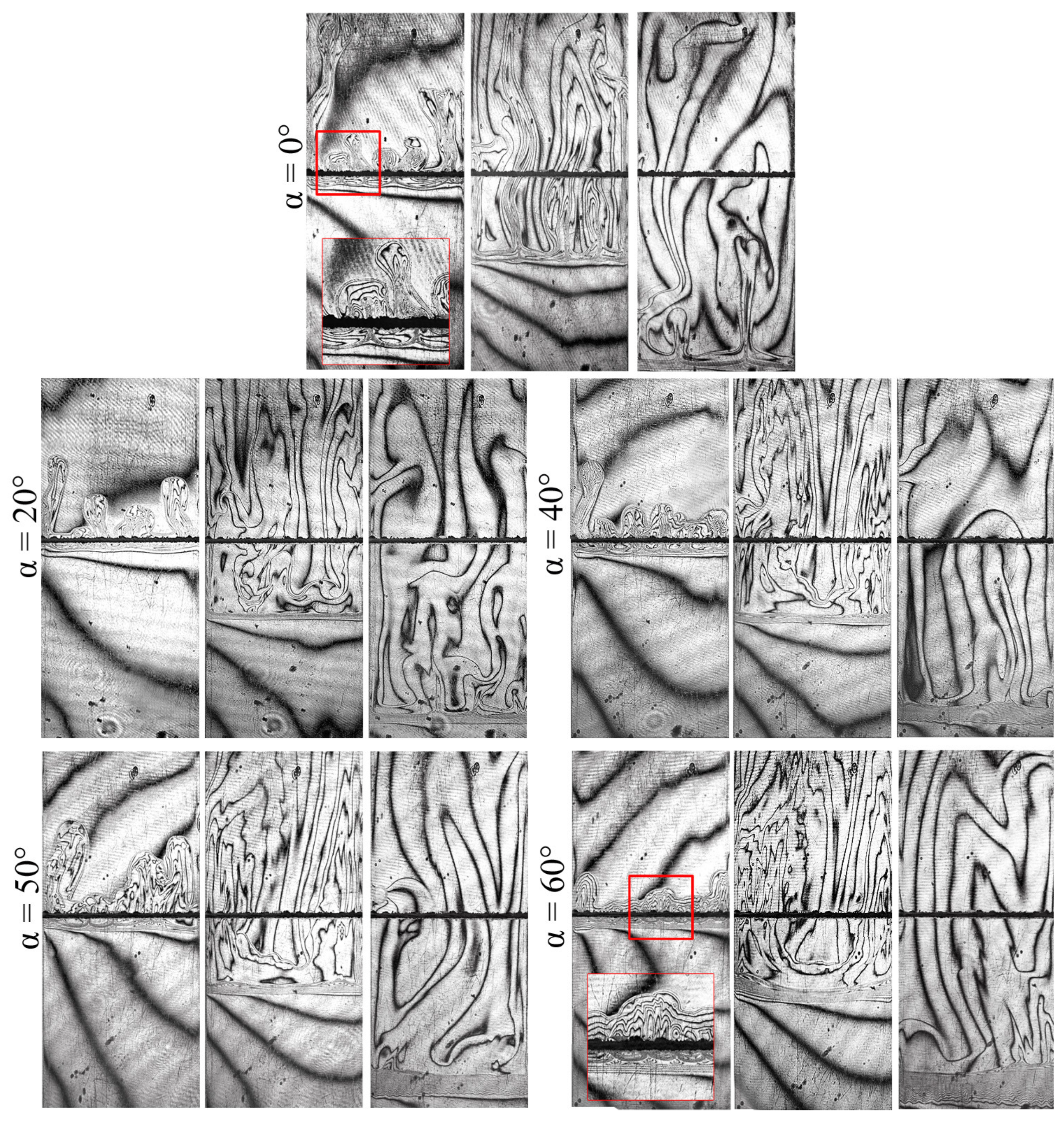
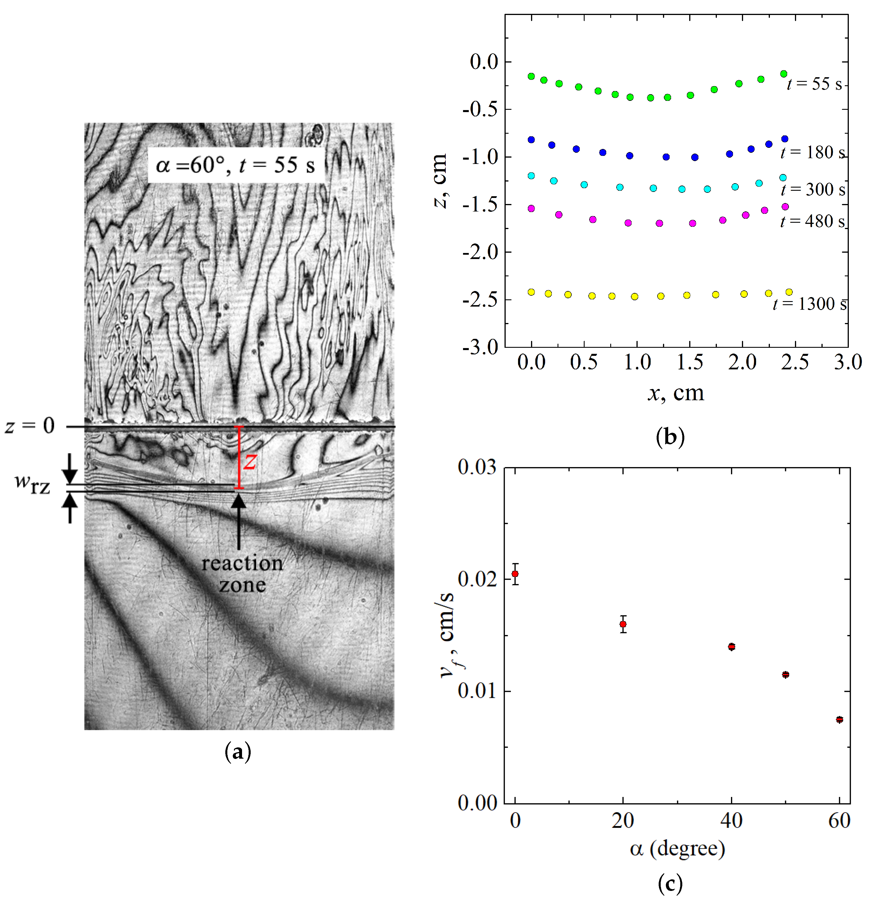
2.2. Experimental Results: Interferogram Analysis

The ratio of the initial concentrations of the reactants is the governing parameter of the reaction–diffusion–convection system we study. It determines the onset of various types of chemoconvection. We choose the initial concentrations from the range when the system evolves in the so-called convection-controlled regime [32]. One observed a shock-like density wave propagating in the direction of gravity force. There was an abrupt change in density and velocity in the moving reaction front, which separated the motionless fluid ahead of it and the area with intensive convective mixing behind it. Our experiments demonstrated that the reactor inclination affected the intensity and structure of convection. It means that the effect also concerns the propagation velocity and the shape of the reaction front.
Figure 3 presents several interferogram sequences, which illustrate how the structure of convective flows changes with a varying inclination angle α . Each series presents three successive interferograms acquired at 7, 180, and 1020 s. In general, the system in the slightly inclined slot ( α > 0 ° ) evolves in the same way as in the case of a vertically oriented cell ( α = 0 ° ). One can observe intense convection in the cocurrent flow above the reaction front and almost motionless fluid below the reaction front. However, a more detailed interferogram analysis has revealed some significant changes.
Let us compare the interferograms at the beginning of the evolution ( t = 7 s) obtained for the different angles. When α = 0 ° , one can observe the active development of convective plumes that rise separately. These plumes arise because of the Rayleigh–Taylor instability driven by the floating of the reaction zone, which is less dense than the upper layer of the system. In case α > 0 ° , the vertical movement of plumes is limited by the upper sidewall of the reactor. Figure 4 schematically illustrates a rising plume in the inclined cavity. By reaching this wall, the plumes unite and spread further in a uniform flow along the front face, moving over the upper layer of the system like intrusion flows [48]. The height of the layer where the plumes can freely rise in the vertical direction decreases with an increase in the inclination angle. Therefore, the time required for the plume intrusion development also reduces. At higher slot inclinations, the intrusion flow becomes noticeable already at an early stage. Figure 3 has two insets marked by the red frame, which illustrate the development of plumes in close-up at α = 0 ° and α = 60 ° . Furthermore, we can learn from Figure 3 that the plumes move separately from each other in a vertically oriented slot, while, in the case of the inclination, they look like a single incoming flow. Since the initial plumes rise at different times and have slightly different velocities, the shape of the propagation front of plume tips is not straight.
Because of the solvent incompressibility, the intrusion of plumes along the upper wall displaces the fluid in the upper layer. This fluid starts to propagate downward along the back wall of the slot. We illustrate this process schematically in Figure 4. The interference pattern that appeared in the middle part of the slot in the form of a downward flow indicates the existence of such a motion (see the series for α > 40 ° in Figure 3). The experiments have shown that the downward flow cannot penetrate through the reaction front into the lower layer and trigger a global mixing of the entire system. The reaction front acts as an impenetrable boundary. By reaching the reaction front, the flow deforms it, turns up, and moves along the upper wall of the slot. As a result, one can observe a large-scale three-dimensional convective motion above the reaction front.
We should notice that when the descending flow turns up near the reaction front, it mixes only with plumes in the central part of the reaction zone. Other plumes are pushed to the lateral boundaries of the slot. As a result, the place where the new plumes appear changes. If, at the beginning of the evolution, the plumes appear over the entire width of the reaction zone at any angle α , then after the onset of three-dimensional convective flow, plumes actively rise only near the lateral cell walls.
The larger the inclination angle, the more the three-dimensional flow affects the shape of the reaction front. The wavefront deformation becomes visible starting from α = 60 ° . To investigate the front deformation, we measured its coordinates using tools of the ImageJ software. Figure 5a schematically shows the measurement process on one typical interferogram. The formation of the product (salt, NaNO 3 ) at the reaction front leads to a sharp change in the value of concentration and, consequently, in the value of the refractive index. Therefore, on the interferogram, the part of the reaction zone with a reaction front is visualized as a contrast band. One can see many closely spaced interference fringes within the band, indicating a large concentration gradient. Since the wavefront is indistinguishable, it is difficult to determine its position accurately. In our measurements, we defined the coordinate of the front position as the distance between z = 0 and the middle of the reaction zone (vertical red line in Figure 5a). To determine the position of the front line, we measured the coordinate z over the entire slot width x. The obtained temporal evolution of the front shape for α = 60 ° is presented in Figure 5b. The error of the measurements was estimated as the ratio of the thickness of the reaction zone w r z to the measured value z. In this case, the significant error will be in measurements carried out for the initial stage of the reaction t < 30 , when the measured value of z differs little from 0. Based on this definition, the measurements made at the beginning of the reaction t < 30 , when the measured value z differs little from 0, will have the maximum possible error. However, we did not analyze this stage of system evolution since the front did not evolve, remaining almost flat. Therefore, we started our measurements from time t > 30 s, when the deformation became significant. The maximum error value did not exceed 2%, which is less than the size of the symbol on the chart (Figure 5b).
As discussed above, at the beginning ( t < 30 s), the three-dimensional flow is just being formed, and the front remains almost flat. After the final formation of the three-dimensional convective motion, the reaction zone becomes concave (see t = 55 s in Figure 5b). With time, the concentration of reactants gradually decreases due to their burning out, and the convection slows down. It results in a decrease in the characteristic value of the intensity of plumes, which is an order of magnitude less than the intensity of plumes forming at the reaction beginning [32]. It means that the 3D convection gradually decays, and the interference pattern in the central part of the cell disappears. The reaction front eventually straightens (see t = 1300 s in Figure 5b), and the convective structure becomes chaotic, which is typical for such reaction systems.
The effect of the “reduction gravity” on the velocity of the reaction front propagation v f is depicted in Figure 5c. We determined this value at the beginning of the reaction evolution when the front was flat and propagated linearly. Using tools of the ImageJ software, we measured the temporal dependence of the reaction zone position z ( t ) and calculated the reaction front velocity v f as a first derivative of z ( t ) . Since the front was flat, the coordinate of the front position was measured only in the central part of the slot, as shown in Figure 5a. We performed at least three experiments for each angle and then averaged obtained values of v f . Error bars in Figure 5c show the standard error. The analysis of the obtained results revealed that an increase in the inclination angle leads to a decrease in the reaction front velocity.

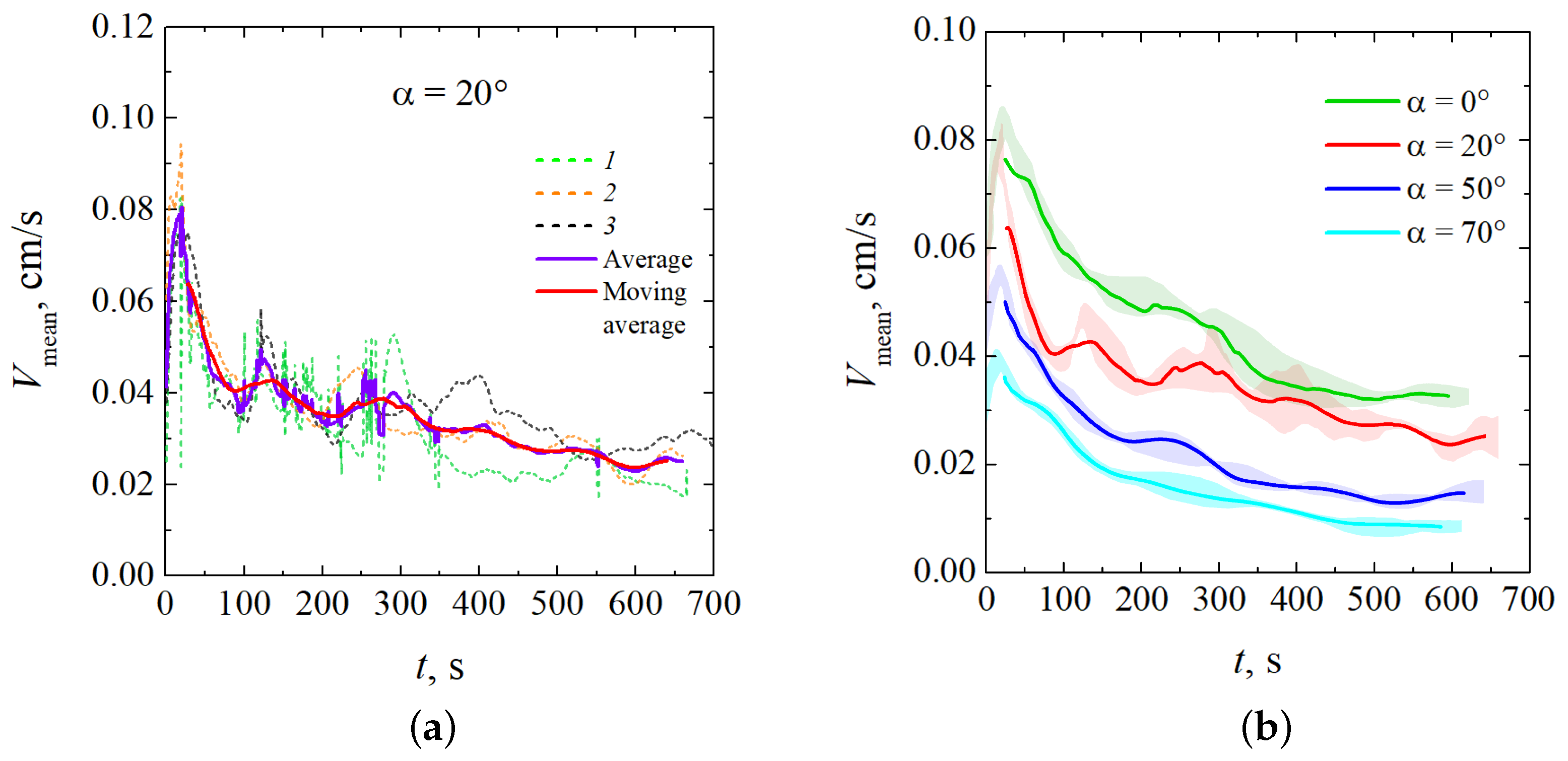
2.3. Experimental Results: PIV Analysis

Quantitative information about the intensity of convection caused by the reaction was obtained using PIV measurements. The experiments were carried out in a thin cell of the same height and thickness as the interferometric cell but had an almost doubled width (5.0 cm). Figure 6 shows the hybrid plots, which include the vector fields of time-average fluid velocity and the color maps of the vorticity fields. It presents two series of plots obtained for α = 0 ° (top row) and α = 70 ° (bottom row). Each series contains frames obtained for successive time moments: 4, 100, and 280 s.
During the system’s evolution, the structure of the reaction-driven convection differs radically. One can observe the formation of elongated disordered convective plumes in a vertically oriented slot. The inclination prevents the free vertical rise of the plumes that become slower. This effect manifests as an ordered row of vortices, regularly spaced along the cell width (Figure 6, t = 4 s).
Further, in the case of an inclined slot, a three-dimensional convective flow develops above the reaction front. In the cross-section, the convection structure consists of three vortices. One vortex appears in the middle part of the cavity, and two smaller ones appear near the lateral boundaries. The vortex structure looks more ordered and differs from those observed in the vertical slot (Figure 6, t = 100 s). The revealed vortex structure remains stable for about two minutes, after which it is gradually distorted by newly rising plumes (Figure 6, t = 280 s). Then, as the reaction slows down ( t > 1000 s), the convection becomes chaotic.
Since we measured PIV in a double-width slab reactor, one could confuse the results presented in Figure 3 and Figure 6 when comparing them. When planning the PIV experiments, we assumed that changing the cell width (while maintaining the same thickness and height) would not lead to noticeable changes in the structure of the convective flow. However, it turned out that the usage of the slot with doubled width led to an increase in the number of vortices of the three-dimensional convection arising above the reaction front. Figure 7 presents a comparison of interferograms obtained for the slots of two different widths. One can see that the interferogram for the narrow slot reveals a downward flow in the central part of the cavity and an upward flow along the side boundaries (Figure 7a). The interferogram of a double-width slot shows just the opposite pattern (Figure 7b). The PIV measurements confirm these observations (Figure 7c). Thus, an increase in the slot width leads to a fragmentation of the three-dimensional convective flow. The further increase in the slot width probably leads to the appearance of a multi-vortex structure.
To characterize the intensity of the reaction-driven convection, we used the mean velocity magnitude, V m e a n extracted from obtained velocity fields. Data obtained from several experimental realizations for α = 20 ° are shown in Figure 8a. One can notice that the value V m e a n continuously fluctuates but still keeps the same order of magnitude. For the convenience of analysis, we averaged the results of several experimental realizations performed under the same conditions. The value of the standard error did not exceed 5%. The resulting average dependence was further smoothed using a moving average calculated with a time window of 25 s. Figure 8b shows smoothed time dependencies of V m e a n for different inclination angles. Shaded regions correspond to the standard errors.
Figure 8 shows that an increase in α also leads to a decrease in the characteristic convection velocity. This result implies the “reduction gravity” effect.

3. Numerical Study

3.1. Mathematical Formulation

As in the experiment, we consider a three-dimensional region filled with aqueous solutions of nitric acid and sodium hydroxide (Figure 1a). The origin of the Cartesian coordinate system is placed at the edge, as shown in the figure. Then the internal cavity is defined by 0 x l , 0 y d , h z h . Thus, we consider a rectangular parallelepiped substantially flattened along the y-axis. We assume that the slot can change its orientation in space concerning gravity.
Given the chosen coordinate system, the gravitational acceleration vector can change its orientation as follows: g = g n , where n is a unit vector with components (0, sin ( α ) , cos ( α ) ). The angle α between the slot walls and the direction of gravity can change from 0 ° (reactor’s vertical position) to 90 ° (reactor’s horizontal position). The initial state includes two well-mixed aqueous solutions of reactants, which, at the very beginning t = 0 , are separated in space by the contact surface z = 0 . After the solutions come into contact, they mix, and the reaction starts. The coefficient k defines the reaction rate. Although the neutralization reaction is exothermal, we consider the problem as isothermal. This assumption is based on the results of our previous works [32,33]. In addition, the wide sidewalls of the slab reactor can always be sufficiently massive and thermally conductive (as in the present study) so that heat diffuses without significant changes in the system dynamics.
For the concentrations of acid A, base B, and their salt S, we write the transport equations as
A t + ( v · ) A = · ( D A ( A ) A ) k A B ,
B t + ( v · ) B = · ( D B ( B ) B ) k A B ,
S t + ( v · ) S = · ( D S ( S ) S ) + k A B .
The neutralization reaction is a non-linear second-order reactive scheme. In this paper, we use the concentration-dependent diffusion model, which we have developed for the aqueous solutions of nitric acid, sodium hydroxide, and their sodium nitrate salt in [33]. As was shown, the model works well until the initial concentrations of reactants do not exceed the value of 3 mol/L:
D A ( A ) 0.881 + 0.158 A , D B ( B ) 0.594 0.087 B , D S ( S ) 0.487 0.284 S .
Thus, the nabla operators in (1)–(3) are applied to the non-linear functions (4). The diffusion terms are written under Fick’s law, which describes how the diffusion rate of components changes with their concentrations.
The results of the experiments demonstrate that if the layer is gradually inclined to gravity, an unsteady spatial flow develops in the slot, and the three-dimensional effects increase with an increase in the inclination angle α . Thus, the Hele–Shaw approximation used in our previous works (see, for example, [33] for more details) now looks like an oversimplification of the problem. Therefore, to obtain the fluid flow, we employ a set of the three-dimensional Navier–Stokes equations written under the Boussinesq approximation for an incompressible fluid [49]:
ρ 0 v t + ( v · ) v = p + η 2 v + ρ g ,
· v = 0 ,
where ρ 0 is the density of the solvent (water), η is the dynamic viscosity, ρ is an increment to the solvent density due to the dissolved reactants and the reaction product:
ρ = β A A + β B R B + β S R S .
We assume that the coefficients of volume expansion β in (7) are constant at low concentration values. According to [32], they are as follows: β A = 0.034 L/mol, β B = 0.043 L/mol, β S = 0.056 L/mol.
Let us now formulate boundary conditions for the problem. We assume that the internal space of the cavity is confined by the solid walls Γ where the velocity becomes zero:
v | Γ   = 0 .
Furthermore, we suppose that there are no fluxes of species through the cavity boundaries:
A m | Γ = 0 , B m | Γ = 0 , S m | Γ = 0 ,
where m is a unit vector normal to the boundary Γ .
Under these assumptions, the initial boundary conditions are as follows:
t = 0 : v = 0 , A = A 0 , z > 0 0 z 0 , B = 0 , z > 0 B 0 z 0 , S = 0 .
The final system of governing equations, boundary, and initial conditions (1)–(10) includes several dimensional parameters such as the reaction rate k and the initial concentrations of reactants A 0 , B 0 . The first parameter is difficult to define accurately. The measurement of the reaction rate in spatially-extended systems requires a separate study. However, as is known, the reaction in these systems proceeds by several orders of magnitude faster than diffusion. In our numerical simulations, we use value k = 10 3 m 3 /(s·mol). The initial concentrations determine the chemoconvection mode [33]. We use values A 0 = 1.8 mol/L, B 0 = 1.5 mol/L, which lead to the development of a shock-wave-like instability.

3.2. Numerical Method

We solved a 3D problem (1)–(10) by using the ANSYS CFX (Canonsburg, PA, USA, license No. 1062978 issued) on the PNRPU high-performance cluster. The laminar character of the fluid flow and the absence of boundary layers make it possible to use a uniform grid. Since the reactor under consideration is significantly compressed in the direction of the y-axis, the aspect ratios of one element of the computational grid Δ x / Δ y and Δ z / Δ y in various simulations ranged from 4.3 to 4.8. In the basic variant, the computational domain 24 × 1.2 × 100 mm was divided into a uniform Cartesian grid with cell size (Hexahedra) 0.35 × 0.08 × 0.35 mm (280,440 Elements). Figure 9a shows the ANSYS meshing in 3D numerical simulations of chemoconvection in a slab reactor.
The core of the numerical scheme included the incompressible fluid model, which is available in ANSYS CFX. The Navier–Stokes equation was supplemented with a source term to describe the buoyancy force. To assemble our numerical scheme to describe chemoconvection in a mixture, we used several basic models integrated into the ANSYS CFX. The first is the laminar flow model (LaminarFlow) based on the Navier–Stokes equations. For aqueous solutions moving at velocities of no more than 1 mm/s in cavities with a characteristic size of 0.01–0.1 m, the Reynolds number does not exceed 10. Therefore, the flow in a slab reactor can be considered a quasi-laminar one with sufficient accuracy.
Another principal model of the ANSYS CFX is MulticomponentFlow. The software allows us to simulate mixtures consisting of an arbitrary number of individual physical components (Species). Each fluid component may have a separate set of physical properties. When calculating fluid flow, the CFX-Solver calculates the corresponding values of the mixture properties for each sample volume in the flow region (Mixture). One assumes that the components are mixed at the molecular level, and the mixture properties depend on the ratio of the ingredients. The ingredients may exist in fixed mass fractions (FixedCompositionMixture) or in variable mass fractions (one can use either VariableCompositionMixture or ReactingMixture). The proportions of each component in mixtures with variable composition may vary in space or time. It can be caused by either the transformation of one substance into another because of a chemical reaction or diffusion and concentration gradients due to the specifics of the boundary and initial conditions.
The solvent velocity is determined by Equation (5). The concentration of solutes evolves according to the transport Equations (1)–(3). The numerical simulation of the mass fraction of the solvent is based on the constraint equation (ConstrainEquation). It is necessary to satisfy the law of mass conservation (the sum of the mass fractions of all components must be equal to one).
To simulate chemoconvection in an isothermal solution, one should set the following properties of liquids: density, dynamic viscosity, and molar mass. In aqueous solutions of small concentration, the solution density depends linearly on its concentration. Therefore, the most suitable approach is the ideal mixture model (IdealMixture), in which the properties of the liquid are calculated based on the proportions of the components. Under the requirements of this model, we include three ingredients (PureSubstance): nitric acid, sodium hydroxide, and sodium nitrate. In addition, we specified one more substance: a multi-component reacting mixture (ReactingMixture), which consists of water, nitric acid, sodium hydroxide, and NaNO 3 salt. The stoichiometric coefficients of all substances are equal to one (Stoichiometric). The reaction rate coefficient was set to 0.001 m 3 /(s mol) [33].
To characterize the intensity of the flow in an inclined reactor, we introduce two integral quantities. The first one is
V a v e ( t ) = h h 0 d 0 l | v | d x d y d z ,
which is the value of the velocity magnitude V a v e ( t ) averaged over the volume of the slot. One should keep in mind that the part of the system located below the reaction front is immobile (at least, at α = 0 ) and does not contribute to the value defined by (11).
Another integral quantity R ( t ) characterizes the total amount of the reaction product in the whole volume of the slot reactor:
R ( t ) = h h 0 d 0 l S ( t , x , y , z ) d x d y d z .
We chose the working grid resolution after the convergence test presented in Figure 9b. This procedure included the calculation of the total amount of the reaction product R ( t ) released into the slot during the first 500 s of the system’s evolution. Numerical experiments were performed on various meshes with element sizes Δ y ranging from 0.06 to 0.15 mm. As we can see from the figure, generally, the total reaction product R changes significantly with successive mesh refinement (more than 40%). However, one can notice that, in the range of 0.1 to 0.06 mm, the change in R does not exceed 3%. Based on these simulation data, we opted for a grid with a single element size of Δ y = 0.08 mm as the main working one.

3.3. Numerical Results

As is known, the vertically oriented slot ( α = 0 ° ) used in the experiments (100 mm high, 24 mm wide, 1.2 mm thick) demonstrates the development of chemoconvective motions, which can be considered quasi-two-dimensional with acceptable accuracy. Thus, such a system perfectly fits to be considered a Hele–Shaw cell. In [33], we developed a simplified mathematical model under the Hele–Shaw approximation. We have shown that, at some initial concentrations of the reactants, the fluid flow is determined by a shock-type density wave propagating in the direction of gravity (see a series of frames for α = 0 ° shown in Figure 10a). Above the density jump (behind the wave), one observes non-stationary convection, which develops in the cocurrent flow. Convective mass transfer feeds the reaction front (it coincides with the wavefront) with fresh acid, supplying it from parts of the medium that are remote from the reaction zone. Below the wavefront (in front of the wave), there is an alkaline solution that is almost immobile (see Figure 10a). Thus, the non-stationary structure resembles a turbulent bore, which sometimes forms on the surface of rivers and reservoirs. This term usually refers to the moving part of a hydraulic jump, the passage of which leaves behind a turbulent fluid on the surface. This analogy is conditional since, in our case, the density wave is internal. We should note that the described structure looks unusual for the Rayleigh–Taylor instability, which usually leads to the development of a fingering convection (for more details, see Refs. [32,33]).
In this work, we experimentally found that the inclination of the slot concerning gravity immediately makes the flow three-dimensional. Let us illustrate this point with the following numerical simulation for a slightly inclined cavity ( α = 30 ° ). Figure 10b shows the temporal dynamics of the density field calculated in the longitudinal cross-section of the slot by plane, which divides the volume into two halves. At first glance, little has changed here compared to Figure 10a. However, Figure 11 more fully reveals the inhomogeneous structure of the flow. It shows the fields of salt and acid concentrations in two different longitudinal cross-sections (in each case, the inset indicates the position of the slot cross-section) at the time t = 50 s after the start of evolution. One should note that the density wave arises because of the development of the Rayleigh–Taylor instability limited by potential barriers. The processes proceeds rapidly, and the movement of the fluid at the 50th second is already a fully developed flow regime. As we can see from the frames (Figure 11a,b), the sections of the layer made at different depths show strikingly different concentration fields. For example, in the cross-section y = 0.2 mm (one-sixth of the slot thickness from the edge), the salt concentration is, on average, low (Figure 11a), and the acid concentration almost reaches its maximum starting value A 0 (Figure 11b). Conversely, in the cross-section y = 1.0 mm (one-sixth of the slot thickness from the other edge), the acid concentration falls ten times, while the salt, on the contrary, reaches its maximum value.
As we can see from Figure 10b and Figure 11, the salt gradually accumulates at the upper wall and finally fills the space between the upper sidewall and the reaction front. It is also worth drawing attention to the dynamic change in the flow type. At t = 50 s, one can see two vortices. Later, at t = 150 s, one observes the development of a four-vortex flow, gradually breaking down its symmetry. With such an inclination of the reactor, the convective wave tail is still strong enough to feed the shock-type wave with fresh acid. The 30 ° slope reduces the intensity of convective processes supporting the wave, but the wavefront still looks planar. In all frames, the reaction front looks more or less straight, and the transition from acidic to alkaline medium occurs very abruptly. We can notice some “fatigue” of the wave in Figure 10b ( t = 600 s), where the wavefront looks slightly blurred. However, it happens at the late stage of the system evolution, when the initial supply of the reactants ends.
It indicates that, in the transverse direction, the concentration field is stratified even at small angles of deviation from the vertical. This conclusion is also valid for velocity and vorticity fields (we discuss the velocity field in more detail below). In the isothermal problem, the concentration effects are primarily responsible for the onset of instability. Thus, apart from the plumes in the cell plane, one can observe circulation in the perpendicular cross-section made above the reaction front. The lightened reaction zone floats up together with the reaction product. Since the slot is inclined, the salt mainly accumulates near the upper boundary, and the solution with acid sinks to the lower wall. We established that such a circulation develops intensively in the first 30–60 s of the system evolution, and then, as the density wave moves downward, it weakens. However, the flow remains three-dimensional up to the complete burnout of the reactants. The discovered additional degree of freedom of the flow indicates the correctness of the problem formulation, including 3D fluid flows.
Let us consider the transfer processes at the inclination angles closer to the horizontal orientation of the slot ( α = 70 ° ). Figure 10c shows the temporal dynamics of the density field calculated in the longitudinal cross-section of the slot by plane, which divides the volume into two halves. In addition, Figure 12 shows the salt and acid concentration fields in the y = 1 mm and y = 0.2 mm cross-sections, respectively. We can see a strong stratification of the fields across the slot. We reconstructed the velocity profiles for this case and found that the flow has a complicated 3D structure (see Figure 13). In some places, the system organizes the upward jet flows of the acid-salt solution along the upper wall of the inclined slot, while, in others, the downward jet flows along the bottom sidewall. As we can see from Figure 13, the fluid velocity can vary in a cross-section across the slot by more than an order of magnitude.
It is worth mentioning two other interesting points. The strong tilting of the cell in the gravitational field causes the reaction front to deform significantly (see Figure 10c and Figure 12). One can see that the density jump blurs, indicating the weakening of convection that supports the reaction. Another pronounced effect concerns the presence of vertical bands in the concentration fields (Figure 12b, t = 120 s). Such a pattern appears at the late stage of the system’s evolution since it demands some time to develop. This pattern looks like a convective concentration instability of the Rayleigh–Bérnard type. The instability develops only near the walls since the central cross-section of the density field by the plane y = 0.6 mm does not demonstrate the development of this pattern (Figure 10c). As is known [50], the first mode of countercurrent instability looks like a periodic system of convective rolls directed toward the flows.
Figure 14 shows the dependencies V a v e (t) for three values of the inclination angle. Hence, one can conclude that the intensity of chemoconvection above the front gradually weakens as α increases. Moreover, the development of the density wave slows down: at α = 0 ° , V a v e reaches its maximum value already at t = 30 s, while, at α = 60 ° , the time increases to t = 120 s. One can see that the changes develop unevenly with increasing angles. Below the angle α = 30 ° , one observes only a weak quantitative effect. At α = 60 ° , the changes are already qualitative (Figure 14). For instance, one can see that the process proceeds more steadily.
Figure 15 shows how the total amount of the reaction product defined by (12) changes over time at different slot inclination angles α . One can notice that the reaction rate depends on the inclination angle non-linearly: at small and medium angles, this dependence manifests itself weakly, while at values close to 90 ° , the system’s susceptibility to the inclination procedure increases sharply.
The considered reaction mechanism with the front moving similar to a shock wave implies a direct relationship between the intensity of convective mixing above the reaction front and the velocity of the reaction front. The experiments and the numerical simulations indicate the following correlation: as the angle of inclination increases, the front velocity decreases. Figure 16 presents the time dependence of the coordinate of the front position x for three values of the inclination angle. The unfilled symbols denote the results of simulations, while the colored ones present the experimental data. The obtained quantitative results are in good agreement.

4. Discussion

One of the applications of phenomena considered in this paper is the control of mass transfer in a continuous-flow microreactor. To mix the reactants in such a reactor, we can use two physical principles: diffusion and convection. When using a diffusion mechanism, one should use a cavity of a smaller cross-section. With the miniaturization of capillaries, the reactor vessel becomes redundant since the reaction occurs in channels. This method is suitable for chemical reactions, which can occur slowly. Another approach implies a special reactor zone, where the convection is applied to mix the species. It leads to an increase in product yield. Today, there are some examples of well-developed technologies to produce pharmaceutical substances in continuous-flow reactors. The literature on this topic is growing quickly, reflecting the interest of researchers.
Let us determine the place of our work in a series of similar studies. The problem considered in this paper is interdisciplinary and has no direct analog. It deals with the processes of convective mass transfer in an inhomogeneous solution complicated by the effects of non-linear diffusion and a second-order reaction occurring in the volume. In addition, the entire system is under the influence of a non-constant gravity tuned by tilting the cavity concerning the acceleration due to gravity. As a rule, similar systems are considered so that only one effect can manifest itself. For example, the problem of the convective stability of a homogeneous fluid filling a vertical layer heated from the side has been studied since the classical works by Gershuni [51] and Batchelor [52]. They showed that the base state is an up-and-down flow generated by 2D thermal convection. Later, Hart [12] found that the inclination of the layer to the gravitational field led to a transition from 2D to 3D convection at tilt angles larger than some critical value (for example, for water, the transition occurred already at α = 1 . 7 c i r c ). Thus, the slightest slope of the vertical layer leads to qualitative changes in the flow structure. A similar effect was observed in the isothermal system [50]. It was a two-layer system of two miscible chemically inert liquids filling a Hele–Shaw cell. Unlike the side-heated vertical layer, the system considered in [50] is symmetrical with respect to horizontal reflection. At the very beginning, the Hele–Shaw cell orients vertically, and the fluid system has a stable density stratification. Then the cavity tilts resulting in an intense 3D Rayleigh–Bénard concentration convection. In this case, the transition to the 3D convection occurs at an arbitrary angle caused by the different densities of the solutions. The works mentioned above motivated us to apply the same technique to our problem.
The chemoconvective regime in the form of a shock wave pattern that we studied both experimentally and numerically in [32,33] accelerates the reaction by two orders of magnitude. Experiments showed that complete burnout of reactants in this regime occurs in a few minutes. Slightly changing the ratio of the initial concentrations of the acid and base, the same process is influenced by the diffusive instabilities and can take several hours. In the case of no convection, the complete burnout of the reactants in the same slot can last even for several days. Thus, turning on the shock-wave mode of the spatial reaction at the right time makes it possible to accelerate the processes tenfold, and turning it off leads to the same slowdown in the rate of burnout of reactants.
In this paper, we considered a simple way to fine-tune the mixing process. If the slot is oriented strictly vertically concerning gravity, then the mechanism of convective mixing in the cocurrent wave flow operates at full strength. We have shown that when the slot is inclined in any direction perpendicular to the slot plane (the original system is symmetrical to these directions), the intensity of chemoconvection gradually decreases. In this case, the effect of the slot inclination is more pronounced with the greater inclination angle. In a horizontal position, the intensity of chemoconvection drastically reduces to a level where a density jump cannot develop at all. In this case, mixing occurs under the control of diffusion.
Our experimental data and the numerical results are in qualitative and quantitative agreement. We found that even a slightly inclined slot demonstrates a transition from quasi-2D chemoconvection, which we can describe using the Hele–Shaw approximation, to full-scale 3D convective motions. Experiment and theory reliably fix the occurrence of spatial flows in the slot, revealing the stratification of salt and acid fields in the direction across the layer. This stratification triggers a global 3D circulation of the solution. The acid is delivered to the reaction front mainly along the lower boundary, while the salt floats near the upper wall. Furthermore, the stratification of the concentration fields leads to secondary instabilities of the up-and-down flow. For example, we recorded the development of a solutal Rayleigh-Bénard instability in the near-wall regions. We should notice that the transition to 3D fluid flow leads to the weakening of the convective mass transfer because the projection of gravity onto the slot plane decreases with the growth of the inclination angle. The phenomenon allows us to fine-tune the mixing intensity by adjusting the inclination angle. Last but not least, the described method to control the mixing process is simple and uses the natural energy of the gravity field.

5. Conclusions

We studied, both experimentally and numerically, the structure of chemoconvection arising in a two-layer system of reacting solutions placed in an inclined slot. The study was performed for a neutralization reaction proceeding, which induces a shock-wave-like structure. We found that such a flow regime persists in the range of inclination angles 0 ° α 60 ° . In this mode, the density wave with a flat front propagates in the direction of the gravity vector at a speed that is an order of magnitude higher than the speed of diffusion processes. The flow in the inclined slot acquires a three-dimensional character. As the angle of inclination increases, the intensity of chemoconvection above the front decreases, and the front propagation speed decreases. The described phenomenon can be used to control the mixing process and fine-tune the reaction rate.

Author Contributions

Conceptualization, E.M. and D.B.; experimental study, E.M.; software, R.S.; validation, R.S. and D.B.; numerical study, R.S.; supervision, D.B.; writing—original draft preparation, E.M. and D.B.; writing—review and editing, D.B.; funding acquisition, D.B. All authors have read and agreed to the published version of the manuscript.

Funding

This research was carried out with the financial support of the Ministry of Science and Higher Education of the Russian Federation in the framework of the program of activities of the Perm Scientific and Educational Center “Rational Subsoil Use”.

Institutional Review Board Statement

Not applicable.

Informed Consent Statement

Not applicable.

Data Availability Statement

The data that support the findings of this study are available from the corresponding author upon reasonable request.

Conflicts of Interest

The authors declare no conflict of interest.

References

  1. Levich, V.G. Physicochemical Hydrodynamics; Prentice-Hall Inc.: Englewood Cliffs, NJ, USA, 1962. [Google Scholar]
  2. Kutepov, A.M.; Polyanin, A.D.; Zapryanov, Z.D.; Vyazmin, A.V.; Kazenin, D.A. Chemical Hydrodynamics: Spravochnoe Posobie; Kvantum: Moscow, Russia, 1996. [Google Scholar]
  3. Dupeyrat, M.; Nakache, E. Direct conversion of chemical energy into mechanical energy at an oil water interface. Bioelectrochemistry Bioenerg. 1978, 5, 134–141. [Google Scholar] [CrossRef]
  4. Belk, M.; Kostarev, K.; Volpert, V.; Yudina, T.M. Frontal photopolymerization with convection. J. Phys. Chem. B 2003, 107, 10292–10298. [Google Scholar] [CrossRef]
  5. Reschetilowski, W. Microreactors in Preparative Chemistry: Practical Aspects in Bioprocessing, Nanotechnology, Catalysis and More; John Wiley & Sons: Hoboken, NJ, USA, 2013. [Google Scholar]
  6. Baumann, M.; Baxendale, I.R. The synthesis of active pharmaceutical ingredients (APIs) using continuous flow chemistry. Beilstein J. Org. Chem. 2015, 11, 1194–1219. [Google Scholar] [CrossRef] [PubMed] [Green Version]
  7. Karlov, S.P.; Kazenin, D.A.; Baranov, D.A.; Volkov, A.V.; Polyanin, D.A.; Vyazmin, A.V. Interphase effects and macrokinetics of chemisorption in the absorption of CO2 by aqueous solutions of alkalis and amines. Russ. J. Phys. Chem. A 2007, 81, 665–679. [Google Scholar] [CrossRef]
  8. Wylock, C.; Rednikov, A.; Haut, B.; Colinet, P. Nonmonotonic Rayleigh-Taylor instabilities driven by gas–liquid CO2 chemisorption. J. Phys. Chem. B 2014, 118, 11323–11329. [Google Scholar] [CrossRef] [Green Version]
  9. Thomson, P.J.; Batey, W.; Watson, R.J. Interfacial activity in the two phase systems UO2(NO3)2/Pu(NO3)4/HNO3-H2O-TBP/OK. In Proceedings of the Extraction’84, Symposium on Liquid–Liquid Extraction Science, Dounreay, Scotland, 27–29 November 1984; Elsevier: Amsterdam, The Netherlands, 1984; Volume 88, pp. 231–244. [Google Scholar]
  10. Gershuni, G. On the problem of stability of plane convective motion of liquids. Zhur. Tekh. Fiz. 1955, 25, 351–357. [Google Scholar]
  11. Birikh, R.; Gershuni, G.; Zhukhovitskii, E.; Rudakov, R. Hydbodynamic and thermal instability of a steady convective flow: PMM vol. 32, no. 2, 1968, pp. 256–263. J. Appl. Math. Mech. 1968, 32, 246–252. [Google Scholar] [CrossRef]
  12. Hart, J.E. Stability of the flow in a differentially heated inclined box. J. Fluid Mech. 1971, 47, 547–576. [Google Scholar] [CrossRef]
  13. Korpela, S.A. A study on the effect of Prandtl number on the stability of the conduction regime of natural convection in an inclined slot. Int. J. Heat Mass Transf. 1974, 17, 215–222. [Google Scholar] [CrossRef]
  14. Linthorst, S.J.M.; Schinkel, W.M.M.; Hoogendoorn, C.J. Flow Structure with Natural Convection in Inclined Air-Filled Enclosures. J. Heat Transf. 1981, 103, 535–539. [Google Scholar] [CrossRef]
  15. Inaba, H. Experimental study of natural convection in an inclined air layer. Int. J. Heat Mass Transf. 1984, 27, 1127–1139. [Google Scholar] [CrossRef]
  16. Bozhko, A.A.; Suslov, S.A. Convection in Ferro-Nanofluids: Experiments and Theory. Physical Mechanisms, Flow Patterns, and Heat Transfer; Springer: Cham, Switzerland, 2018. [Google Scholar]
  17. Gershuni, G.Z.; Lyubimov, D.V. Thermal Vibrational Convection; Wiley: Hoboken, NJ, USA, 1998; p. 376. [Google Scholar]
  18. Mialdun, A.; Ryzhkov, I.I.; Melnikov, D.E.; Shevtsova, V. Experimental evidence of thermal vibrational convection in a nonuniformly heated fluid in a reduced gravity environment. Phys. Rev. Lett. 2003, 101, 084501. [Google Scholar] [CrossRef] [PubMed] [Green Version]
  19. Gaponenko, Y.; Shevtsova, V. Effects of vibrations on dynamics of miscible liquids. Acta Astronaut. 2010, 66, 174–182. [Google Scholar] [CrossRef] [Green Version]
  20. Gaponenko, Y.; Shevtsova, V. Shape of diffusive interface under periodic excitations at different gravity levels. Microgravity Sci. Technol. 2016, 28, 431–439. [Google Scholar] [CrossRef]
  21. Zyuzgin, A.V.; Putin, G.F.; Ivanova, N.G.; Chudinov, A.V.; Ivanov, A.I.; Kalmykov, A.V.; Polezhaev, V.I.; Emelianov, V.M. The heat convection of near critical fluid in the controlled microacceleration field under zero-gravity condition. Adv. Space Res. 2003, 32, 205–210. [Google Scholar] [CrossRef]
  22. Zyuzgin, A.V.; Putin, G.F.; Kharisov, A.F. Ground Modeling of Thermovibrational Convection in Real Weightlessness. Fluid Dyn. 2007, 42, 354–361. [Google Scholar] [CrossRef]
  23. Bratsun, D.A.; Teplov, V.S. On the stability of the pulsed convective flow with small heavy particles. Eur. Phys. J. A. P. 2000, 10, 219–230. [Google Scholar] [CrossRef]
  24. Bratsun, D.A. Effect of unsteady forces on the stability of non-isothermal particulate flow under finite-frequency vibrations. Microgravity Sci. Technol. 2009, 21, 153–158. [Google Scholar] [CrossRef]
  25. Wolf, G.G.H. Dynamic stabilization of the Rayleigh-Taylor instability of miscible liquids and the related “frozen waves”. Phys. Fluids 2018, 30, 021701. [Google Scholar] [CrossRef] [Green Version]
  26. Kozlov, N. Numerical investigation of double-diffusive convection at vibrations. J. Phys. Conf. Ser. 2021, 1809, 012023. [Google Scholar] [CrossRef]
  27. Ivanova, A.A.; Kozlov, V.G. Vibrational Convection in a Nontranslationally Oscillating Cavity (Isothermal Case). Fluid Dyn. 2003, 38, 186–192. [Google Scholar] [CrossRef]
  28. Kozlov, V.G.; Kozlov, N.V.; Subbotin, S. The effect of oscillating force field on the dynamics of free inner core in a rotating fluid-filled spherical cavity. Phys. Fluids 2015, 27, 124101. [Google Scholar] [CrossRef]
  29. Hu, H.Y.; Wang, Z.H. Dynamics of Controlled Mechanical Systems with Delayed Feedback; Springer: Berlin-Heidelberg, Germany; New York, NY, USA, 2002; p. 294. [Google Scholar]
  30. Bratsun, D.A.; Krasnyakov, I.V.; Zyuzgin, A.V. Active control of thermal convection in a rectangular loop by changing its spatial orientation. Microgravity Sci. Technol. 2018, 30, 43–52. [Google Scholar] [CrossRef]
  31. Bratsun, D.A.; Mosheva, E.A. Peculiar properties of density wave formation in a two-layer system of reacting miscible liquids. Comput. Contin. Mech. 2018, 11, 302–322. [Google Scholar] [CrossRef]
  32. Mizev, A.; Mosheva, E.; Bratsun, D. Extended classification of the buoyancy-driven flows induced by a neutralization reaction in miscible fluids. Part 1. Experimental study. J. Fluid Mech. 2021, 916, A22. [Google Scholar] [CrossRef]
  33. Bratsun, D.; Mizev, A.; Mosheva, E. Extended classification of the buoyancy-driven flows induced by a neutralization reaction in miscible fluids. Part 2. Theoretical study. J. Fluid Mech. 2021, 916, A23. [Google Scholar] [CrossRef]
  34. Loodts, V.; Thomas, C.; Rongy, L.; De Wit, A. Control of convective dissolution by chemical reactions: General classification and application to CO2 dissolution in reactive aqueous solutions. Phys. Rev. Lett. 2014, 113, 114501. [Google Scholar] [CrossRef] [PubMed] [Green Version]
  35. Bratsun, D.; Siraev, R. Controlling mass transfer in a continuous-flow microreactor with a variable wall relief. Int. Commun. Heat Mass Transf. 2020, 113, 104522. [Google Scholar] [CrossRef]
  36. Howle, L.E. Control of Rayleigh-Bénard convection in a small aspect ratio container. Int. J. Heat Mass Transf. 1997, 40, 817–822. [Google Scholar] [CrossRef]
  37. Burgess, J.M.; Juel, A. snd McCormick, W.D.; Swift, J.B.; Swinney, H.L. Suppression of dripping from a ceiling. Phys. Rev. Lett. 2001, 86, 1203–1206. [Google Scholar] [CrossRef] [Green Version]
  38. Garnier, N.; Grigoriev, R.O.; Schatz, M.F. Optical Manipulation of Microscale Fluid Flow. Phys. Rev. Lett. 2003, 91, 054501. [Google Scholar] [CrossRef] [PubMed] [Green Version]
  39. Rogers, B.N.; Dorland, W.; Kotschenreuther, M. Generation and Stability of Zonal Flows in Ion-Temperature-Gradient Mode Turbulence. Phys. Rev. Lett. 2000, 85, 5336–5339. [Google Scholar] [CrossRef] [PubMed]
  40. Eckert, K.; Rongy, L.; De Wit, A. A+ B → C reaction fronts in Hele-Shaw cells under modulated gravitational acceleration. Phys. Chem. Chem. Phys. 2012, 14, 7337–7345. [Google Scholar] [CrossRef] [Green Version]
  41. Mosheva, E.; Kozlov, N. Study of chemoconvection by PIV at neutralization reaction under normal and modulated gravity. Exp. Fluids 2021, 62, 1–13. [Google Scholar] [CrossRef]
  42. Bratsun, D.A.; Stepkina, O.S.; Kostarev, K.G.; Mizev, A.I.; Mosheva, E.A. Development of concentration-dependent diffusion instability in reactive miscible fluids under influence of constant or variable inertia. Microgravity Sci. Technol. 2016, 28, 575–585. [Google Scholar] [CrossRef]
  43. Utochkin, V.Y.; Siraev, R.R.; Bratsun, D.A. Pattern Formation in Miscible Rotating Hele-Shaw Flows Induced by a Neutralization Reaction. Microgravity Sci. Technol. 2021, 33, 1–20. [Google Scholar] [CrossRef]
  44. Nikolsky, B.N. (Ed.) Spravochnik Khimika (Chemist’s Handbook), 2nd ed.; Khimiya Publishing House: Moscow, Russia, 1965; Volume 3. [Google Scholar]
  45. Thielicke, W.; Stamhuis, E. PIVlab–towards user-friendly, affordable and accurate digital particle image velocimetry in MATLAB. J. Open Res. Softw. 2014, 2. [Google Scholar] [CrossRef] [Green Version]
  46. Kozlov, N. Images Batch Rotation. 2022. Available online: https://www.mathworks.com/matlabcentral/fileexchange/112590-images-batch-rotation (accessed on 17 February 2022).
  47. Kozlov, N. Images Batch Rotation. 2023. Available online: https://www.mathworks.com/matlabcentral/fileexchange/121682-pivlab_batch (accessed on 17 February 2022).
  48. Schöpf, W.; Stiller, O. Three-dimensional patterns in a transient, stratified intrusion flow. Phys. Rev. Lett. 1997, 79, 4373. [Google Scholar] [CrossRef]
  49. Landau, L.D.; Lifshits, E.M. Fluid Mechanics; Butterworth-Heinemann: Oxford, UK, 1987; p. 560. [Google Scholar]
  50. Mizev, A.; Mosheva, E.; Kostarev, K.; Demin, V.; Popov, E. Stability of solutal advective flow in a horizontal shallow layer. Phys. Rev. Fluids 2017, 2, 103903. [Google Scholar] [CrossRef]
  51. Gershuni, G.Z. On the stability of plane-parallel convective fluid flow. Zh. Tech. Fiz. 1953, 23, 1838–1844. [Google Scholar]
  52. Batchelor, G.K. Heat transfer by free convection across a closed cavity between vertical boundaries at different temperatures. Quart. Appl. Math. 1954, 12, 209–233. [Google Scholar] [CrossRef] [Green Version]
Figure 1. (a) Schematic diagram of an experimental two-layer system of miscible liquids filling a rectangular slot inclined at an angle α to gravity. The green frame in the right image indicates the location of the laser sheet plane. (b) Photo of the general view of the laboratory setup: 1—the rectangular interferometric cell with a two-layer system; 2—a mirror that makes it possible to obtain a reflected light interferometry image; 3—the rotary system for changing the angle of inclination of the experimental cell.
Fluids 08 00098 g001
Figure 2. Stages of the velocity field determination for α = 70 ° . (a) The image demonstrates particle distribution at t = 200 s. The red frame shows the Region of Interest (ROI) for which the velocity field was calculated, and the shaded red areas show the mask applied to regions with shadows cast by the setup parts. (b) Superimposed image demonstrating the particle distribution and the corresponding vector field of the time-average fluid velocity calculated by PIV for time t = 200 s. (c) The vector plot of the time-average fluid velocity. The density plot presents the scalar field of the average velocity magnitude.
Fluids 08 00098 g002
Figure 3. Five series of interferograms demonstrating the dynamic development of the chemoconvective flow at different angles of the slot inclination. Each series contains three frames obtained for consecutive times: 7, 180, and 1020 s.
Fluids 08 00098 g003
Figure 4. Schematic presentation of the slab reactor illustrating the effect of its inclination on the dynamics of the reaction zone (marked by yellow).
Fluids 08 00098 g004
Figure 5. (a) Scheme of the measurement of the front position coordinate. (b) Temporal evolution of the shape of the reaction front in ( x , z ) -plane shown for α = 60 ° . The line z = 0 cm corresponds to the initial contact surface between reacting solutions. (c) Velocity magnitude of the reaction front as a function of the inclination angle α .
Fluids 08 00098 g005
Figure 6. Time evolution of the vector plot of the time-average fluid velocity obtained by PIV at α = 0 ° (top row) and α = 70 ° (bottom row). The color maps represent the vorticity of the time-averaged velocity. The slot width is 5 cm. Each row presents the plots obtained for successive times: 4, 100, and 280 s.
Fluids 08 00098 g006
Figure 7. Comparison of the convective structure developing at α = 70 ° in an inclined slot with single (a) and doubled (b,c) widths. The hybrid plot in (c) presents the vorticity (indicated by the color map) and the time-average velocity (indicated by the vector field). Time after the experiment onset: (a) 240 s; (b,c) 100 s.
Fluids 08 00098 g007
Figure 8. Temporal evolution of the characteristic velocity, V m e a n : (a) the comparison of three experimental realizations performed for α = 20 ° with their average and moving average; (b) the comparison of the results obtained for different inclination angles.
Fluids 08 00098 g008
Figure 9. (a) The ANSYS meshing in 3D numerical simulations of the chemoconvective flow in a slab reactor, the computational grid with 300 × 15 × 1250 cells is shown; (b) the convergence test of the total reaction product R ( t ) released during the first 500 s of flow evolution in a vertically oriented reactor with gradual grid refinement. Δ y stands for the cell size in the y direction. When refining the grid, the cell element (hexahedron) decreases proportionally.
Fluids 08 00098 g009
Figure 10. The density fields calculated for the inclination angles α = 0 ° (a); α = 30 ° (b); α = 70 ° (c). The frames of each series from left to right correspond to the successive times y = 10 s; 50 s; 150 s; 600 s, respectively. A contrast color palette was used to reveal the fine structure of the density fields. All fields are represented in the longitudinal section of the slot by plane y = 0.6 mm, which divides the volume exactly into halves. The red line in the inset indicates the cross-section of the slot where the concentration distribution is shown.
Fluids 08 00098 g010
Figure 11. The concentration field of the reaction product S (a) and the acid A (b) for the inclination angle α = 30 ° shown at t = 50 s. The salt and acid concentration fields are marked in red and green, respectively. The frames from left to right correspond to the layer cross-sections y = 0.2 and 1.0 mm. The red line in the inset indicates the cross-section of the slot where the concentration distribution is shown. A dashed line indicates the initial front of the reaction.
Fluids 08 00098 g011
Figure 12. The concentration fields of the reaction product S in the y = 1 mm cross-section (a) and the acid A in the y = 0.2 mm cross-section (b) for three successive times t = 30 ; 120; 600 s. The inclination angle with respect to the gravity vector is α = 70 ° . The salt and acid concentration fields are marked in red and green, respectively. The red line in the inset indicates the cross-section of the slot where the concentration distribution is shown. A dashed line indicates the reaction front.
Fluids 08 00098 g012
Figure 13. The velocity profiles calculated at time t = 50 s in two cross-sections x = 3 mm ( Γ 1 ) and x = 9 mm ( Γ 2 ). The inclination angle α = 70 ° . Maximum velocity found in the cross-sections Γ 1 and Γ 2 is 0.2 cm/s. The red line shows the trajectory of the main fluid jet.
Fluids 08 00098 g013
Figure 14. Temporal evolution of a domain-averaged convection velocity measured at different inclination angles of the slot.
Fluids 08 00098 g014
Figure 15. Temporal evolution of the amount of the reaction product R ( t ) measured at different inclination angles of the slot.
Fluids 08 00098 g015
Figure 16. Dependence of the position of the wavefront on time for three values of the angle of inclination α = 0 ° (indicated by the black squares), α = 20 ° (red circles), α = 60 ° (blue triangles). The filled and unfilled symbols correspond to the experimental data and the results of numerical simulations, respectively.
Fluids 08 00098 g016
Disclaimer/Publisher’s Note: The statements, opinions and data contained in all publications are solely those of the individual author(s) and contributor(s) and not of MDPI and/or the editor(s). MDPI and/or the editor(s) disclaim responsibility for any injury to people or property resulting from any ideas, methods, instructions or products referred to in the content.

