

Simulation of Particulate Matter Structure Detachment from Surfaces of Wall-Flow Filters for Elevated Velocities Applying Lattice Boltzmann Methods

Abstract
:1. Introduction
2. Mathematical Modelling and Numerical Methods
2.1. Lattice Boltzmann Method
2.2. Porous Media Modelling
2.3. Surface-Resolved Particle Simulations
2.4. Quantification of Errors and Convergence
3. Application to a Wall-Flow Filter
- 1.
- Particle-free flow
- 2.
- Single layer fragment
- 3.
- Deposition layer during break-up
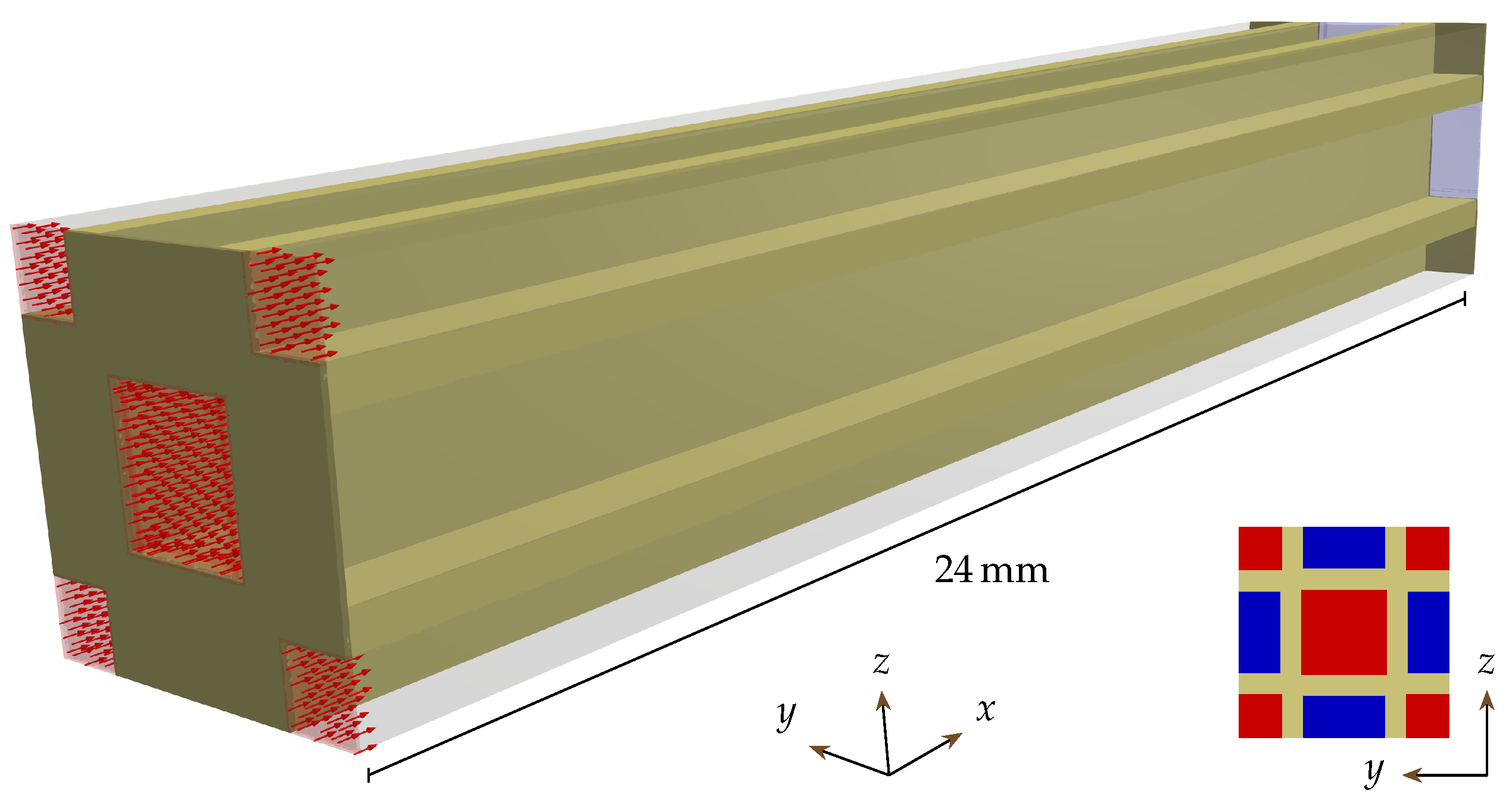
3.1. Particle-Free Flow
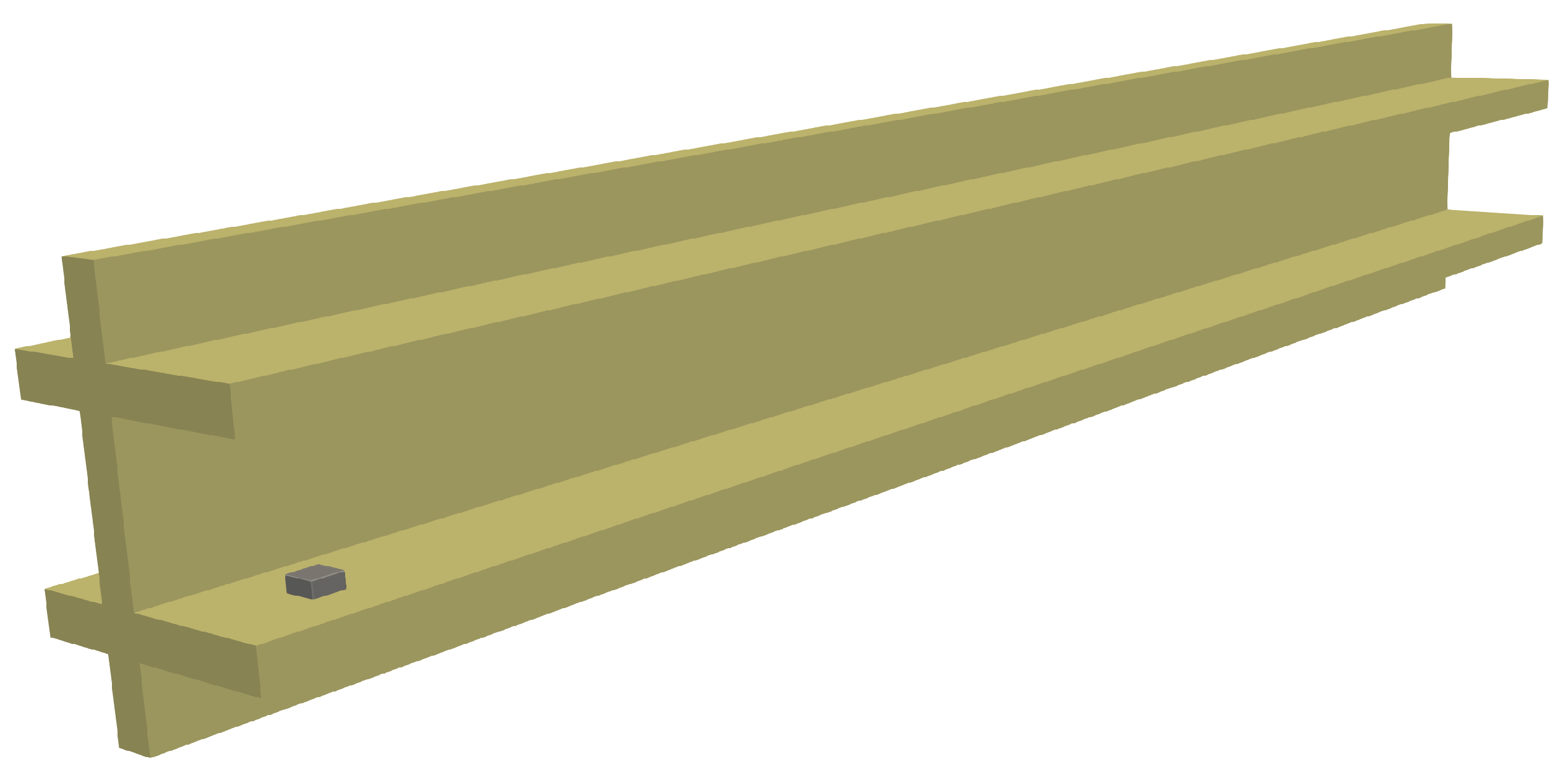
3.2. Single Deposition Layer Fragment
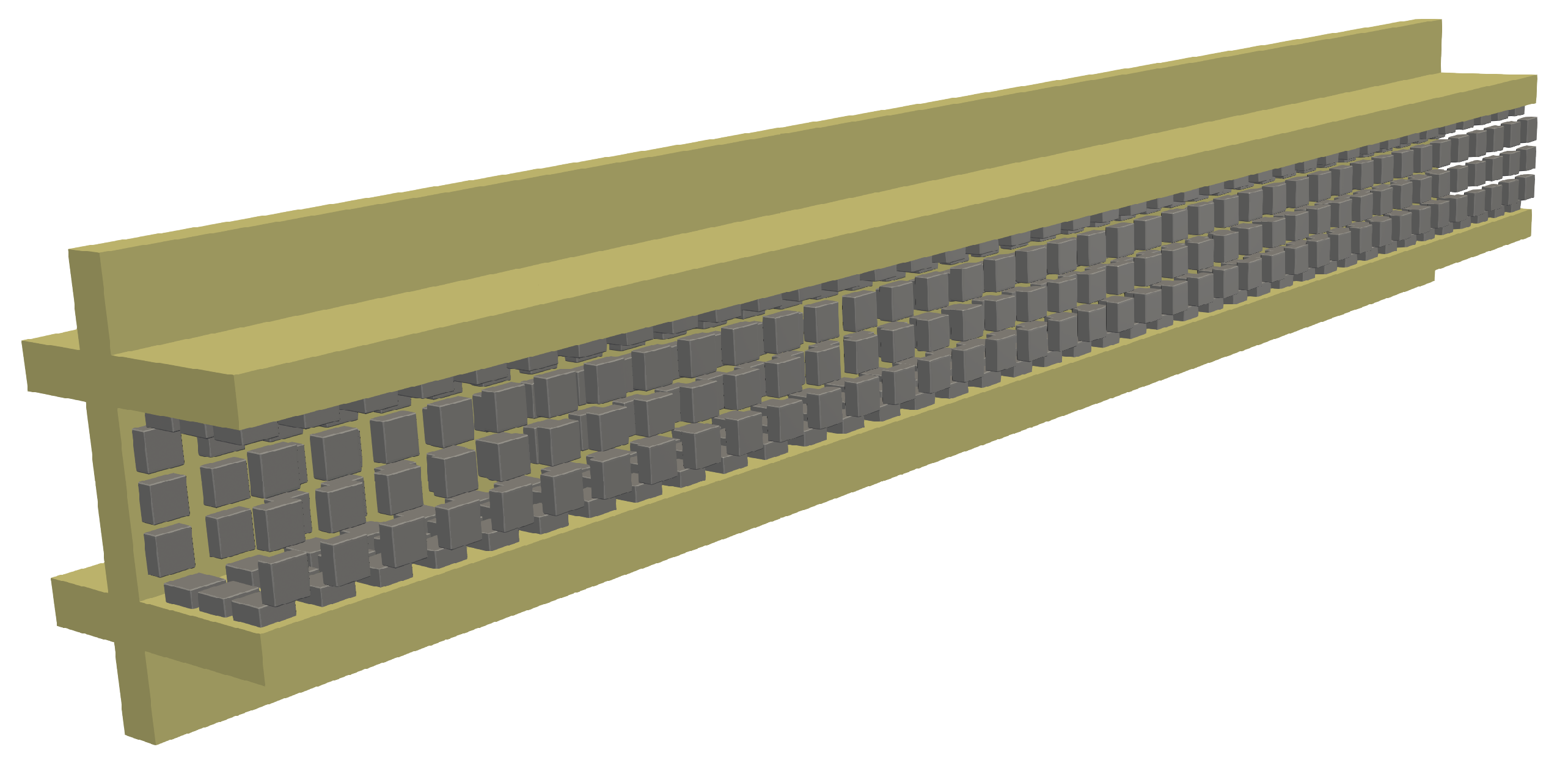
3.3. Deposition Layer during Break-Up
4. Results and Discussion
4.1. Particle-Free Flow
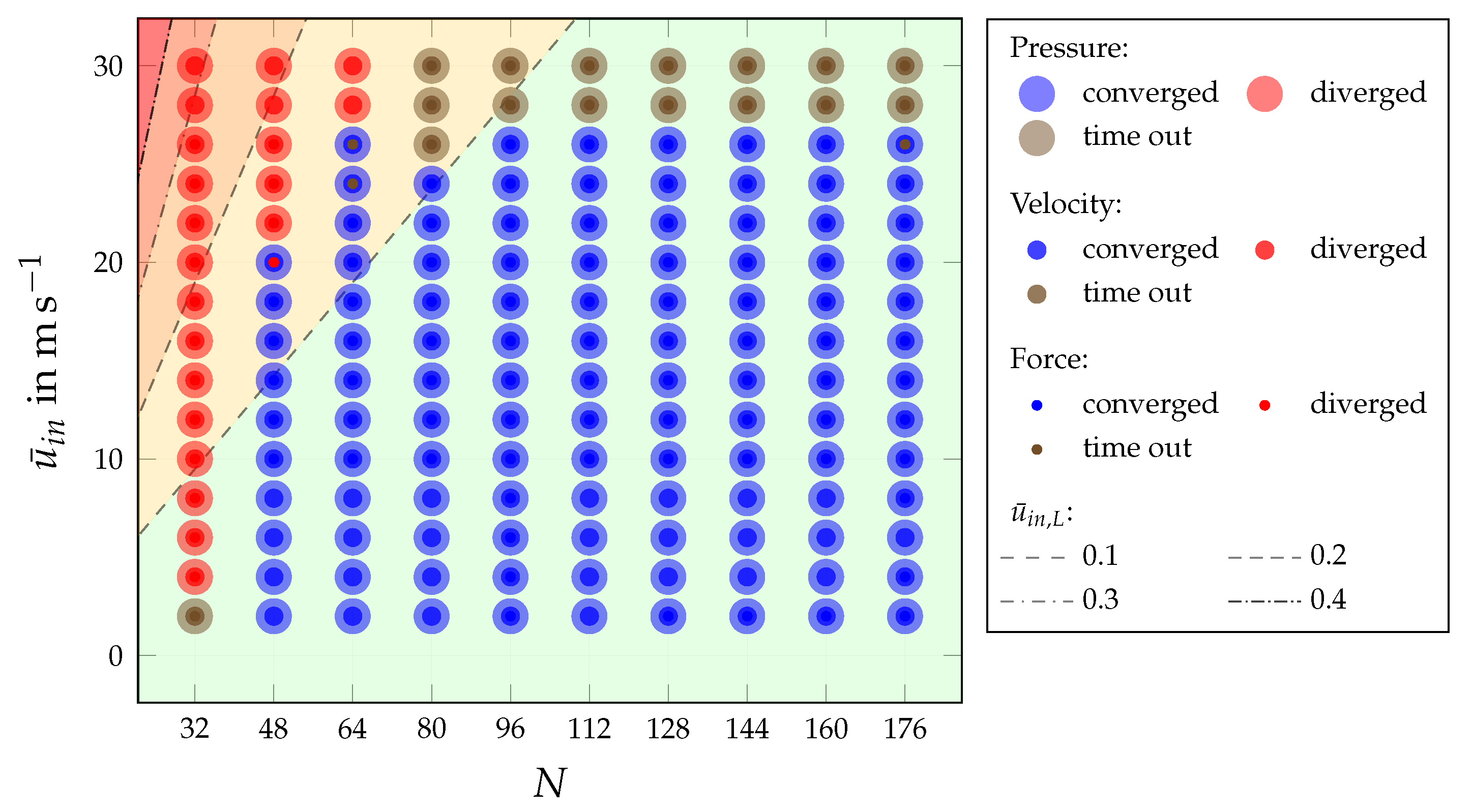
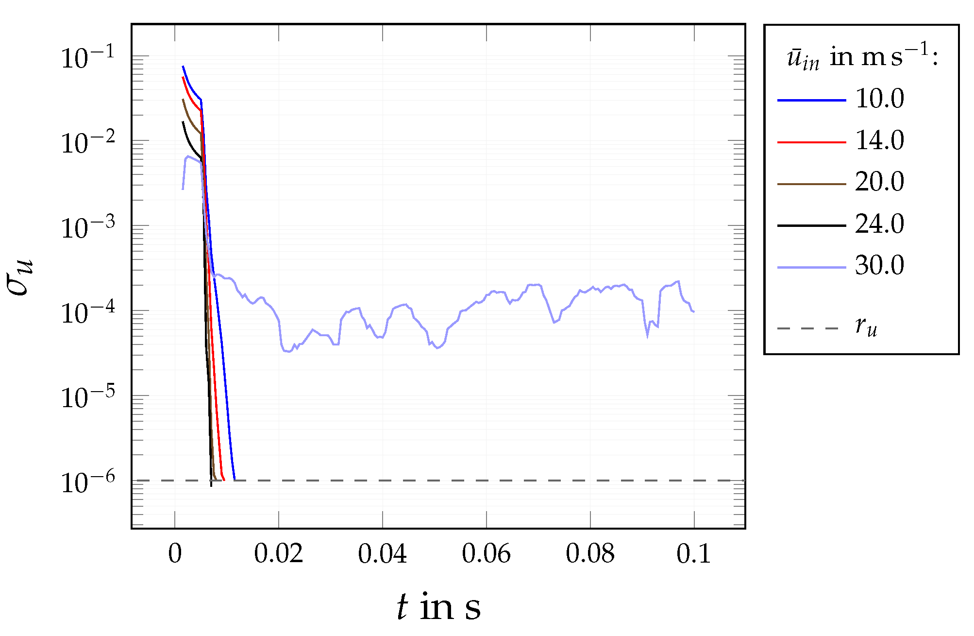
4.1.1. Transient Convergence Behaviour
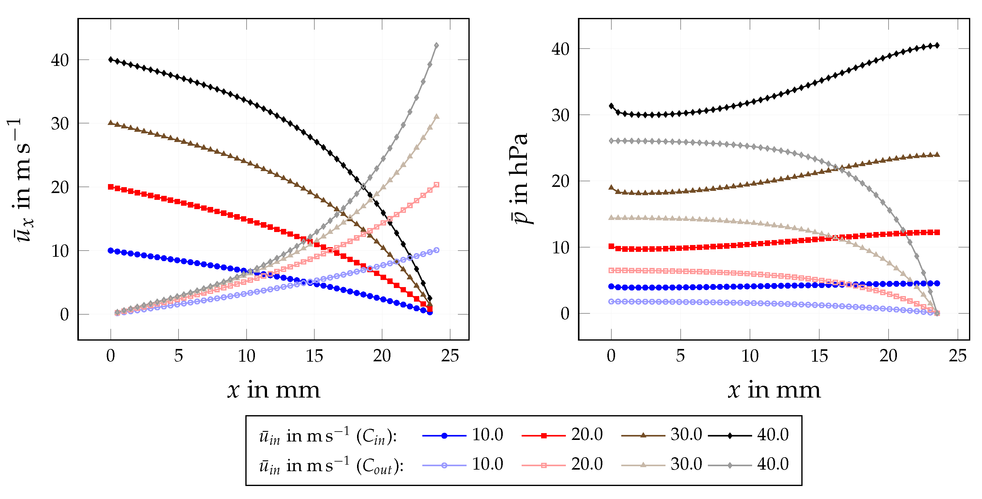
4.1.2. Flow Field
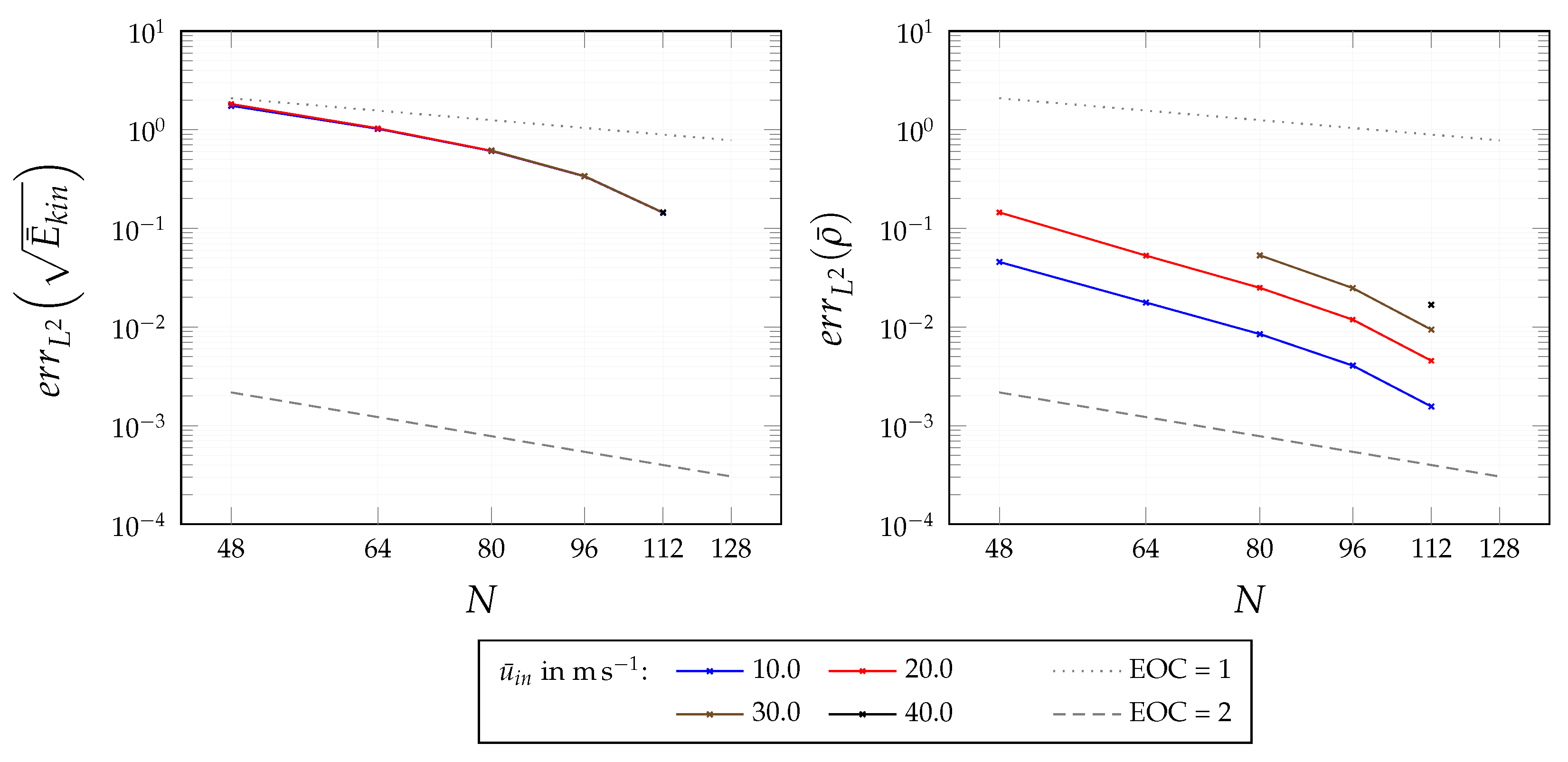
4.1.3. Grid Convergence
4.2. Single Deposition Layer Fragment
4.2.1. Transient Convergence Behaviour
4.2.2. Flow Field
4.2.3. Grid Convergence
4.3. Deposition Layer during Break-Up
4.3.1. Uniformly Fragmented Deposition Layer
4.3.2. Influence of Uniform Layer Height
4.3.3. Influence of Increasing Layer Height
4.3.4. Influence of Non-Uniform Layer Fragmentation
4.3.5. Influence of Partial Detachment
5. Conclusions
Author Contributions
Funding
Data Availability Statement
Acknowledgments
Conflicts of Interest
Abbreviations and Nomenclature
Abbreviations
| BGK | Bhatnagar–Gross–Krook |
| EOC | experimental order of convergence |
| FVM | finite volume method |
| HLBM | homogenized lattice Boltzmann method |
| LBE | lattice Boltzmann equation |
| LBM | lattice Boltzmann method |
| NSE | Navier–Stokes equation |
| PM | particulate matter |
| PSM | partially saturated method |
Nomenclature
| fluid velocity | distance to wall at peak velocity | ||
| p | fluid pressure | distance to wall at starting position | |
| fluid density | stopping distance | ||
| kinematic fluid viscosity | drag force | ||
| position | diameter of reference sphere | ||
| t | time | generic flow quantity | |
| discrete spacing of voxel mesh | average of generic flow quantity | ||
| discrete time step | standard deviation of flow quantity | ||
| N | resolution of voxel mesh | r | residuum of flow quantity |
| D | number of spacial dimensions | T | number of last time steps |
| q | number of discrete velocities | M | total cell number |
| discrete velocity | channel length | ||
| f | distribution function | channel width | |
| discrete-velocity distribution function | channel height | ||
| discrete-velocity equilibrium distribution function | length scaling factor | ||
| discrete collision operator | scaled channel length | ||
| lattice relaxation time | average inflow velocity | ||
| weight of discrete lattice velocity | average wall penetrating velocity | ||
| lattice speed of sound | particle starting position (before detachment) | ||
| K | permeability | initial force (before detachment) | |
| minimum permeability | particle density | ||
| d | confined permeability | number of cells | |
| effective velocity | fragment’s x-dimension | ||
| B | local weighting factor | fragment’s y-dimension | |
| velocity at solid particle node | fragment’s z-dimension | ||
| k | particle index | fragment’s x- and y-dimension | |
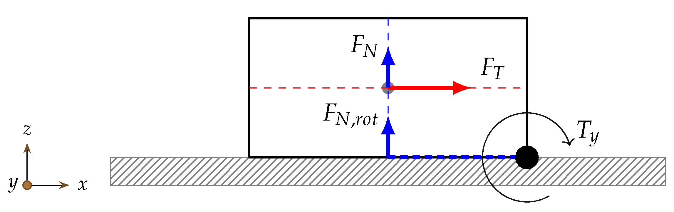
| particle’s centre of mass | rotation-induced normal force | ||
| point on outward-facing normal of surface | relative position along channel length | ||
| width of smooth transition layer | number of particles | ||
| position of discrete particle boundary node | number of particles over channel width | ||
| force acting on particle’s centre of mass | number of particles over channel length | ||
| torque acting on particle’s centre of mass | maximum simulation time | ||
| particle mass | inlet channel domain | ||
| initial particle velocity | outlet channel domain | ||
| relative particle velocity w. r. t. fluid |
References
- Wang, Y.; Kamp, C.J.; Wang, Y.; Toops, T.J.; Su, C.; Wang, R.; Gong, J.; Wong, V.W. The origin, transport, and evolution of ash in engine particulate filters. Appl. Energy 2020, 263, 114631. [Google Scholar] [CrossRef]
- Gaiser, G. Berechnung von Druckverlust, Ruß- und Ascheverteilung in Partikelfiltern. MTZ Mot. Z. 2005, 66, 92–102. [Google Scholar] [CrossRef]
- Sappok, A.; Govani, I.; Kamp, C.; Wang, Y.; Wong, V. In-Situ Optical Analysis of Ash Formation and Transport in Diesel Particulate Filters During Active and Passive DPF Regeneration Processes. SAE Int. J. Fuels Lubr. 2013, 6, 336–349. [Google Scholar] [CrossRef]
- Ishizawa, T.; Yamane, H.; Satoh, H.; Sekiguchi, K.; Arai, M.; Yoshimoto, N.; Inoue, T. Investigation into Ash Loading and Its Relationship to DPF Regeneration Method. SAE Int. J. Commer. Veh. 2009, 2, 164–175. [Google Scholar] [CrossRef]
- Aravelli, K.; Heibel, A. Improved Lifetime Pressure Drop Management for Robust Cordierite (RC) Filters with Asymmetric Cell Technology (ACT). In Proceedings of the SAE World Congress & Exhibition, Nottingham, UK, 20–24 May 2007; SAE International: Warrendale, PA, USA, 2007. [Google Scholar] [CrossRef] [Green Version]
- Dittler, A. Ash Transport in Diesel Particle Filters. In Proceedings of the SAE 2012 International Powertrains, Fuels & Lubricants Meeting, Malmo, Sweden, 18–20 September 2012; SAE International: Warrendale, PA, USA, 2012. [Google Scholar] [CrossRef]
- Dittler, A. Abgasnachbehandlung mit Partikelfiltersystemen in Nutzfahrzeugen, 1st ed.; Wuppertaler Reihe zur Umweltsicherheit, Shaker: Herzogenrath, Germany, 2014. [Google Scholar]
- Wang, Y.; Kamp, C. The Effects of Mid-Channel Ash Plug on DPF Pressure Drop. In Proceedings of the SAE 2016 World Congress and Exhibition, Detroit, MI, USA, 12–14 April 2016; SAE International: Warrendale, PA, USA, 2016. [Google Scholar] [CrossRef]
- Hafen, N.; Dittler, A.; Krause, M.J. Simulation of particulate matter structure detachment from surfaces of wall-flow filters applying lattice Boltzmann methods. Comput. Fluids 2022, 239, 105381. [Google Scholar] [CrossRef]
- Konstandopoulos, A.G.; Skaperdas, E.; Warren, J.; Allansson, R. Optimized Filter Design and Selection Criteria for Continuously Regenerating Diesel Particulate Traps. In Proceedings of the International Congress & Exposition, Fort Lauderdale, FL, USA, 6–8 December 1999; SAE International: Warrendale, PA, USA, 1999. [Google Scholar] [CrossRef]
- Hafen, N.; Thieringer, J.R.; Meyer, J.; Krause, M.J.; Dittler, A. Numerical investigation of detachment and transport of particulate structures in wall-flow filters using lattice Boltzmann methods. J. Fluid Mech. 2023, 956, A30. [Google Scholar] [CrossRef]
- Thieringer, J.R.D.; Hafen, N.; Meyer, J.; Krause, M.J.; Dittler, A. Investigation of the Rearrangement of Reactive ash; Inert Particulate Structures in a Single Channel of a Wall-Flow Filter. Separations 2022, 9, 195. [Google Scholar] [CrossRef]
- Krüger, T.; Kusumaatmaja, H.; Kuzmin, A.; Shardt, O.; Silva, G.; Viggen, E.M. The Lattice Boltzmann Method—Principles and Practice; Springer: Cham, Switzerland, 2016. [Google Scholar] [CrossRef]
- Ferziger, J.H.; Perić, M. Numerische Strömungsmechanik; Springer: Berlin/Heidelberg, Germany, 2008. [Google Scholar] [CrossRef]
- Brinkman, H.C. A calculation of the viscous force exerted by a flowing fluid on a dense swarm of particles. Flow Turbul. Combust. 1949, 1, 27. [Google Scholar] [CrossRef]
- Bhatnagar, P.L.; Gross, E.P.; Krook, M. A Model for Collision Processes in Gases. I. Small Amplitude Processes in Charged and Neutral One-Component Systems. Phys. Rev. 1954, 94, 511–525. [Google Scholar] [CrossRef]
- Ginzburg, I. Equilibrium-type and link-type lattice Boltzmann models for generic advection and anisotropic-dispersion equation. Adv. Water Resour. 2005, 28, 1171–1195. [Google Scholar] [CrossRef]
- Simonis, S.; Haussmann, M.; Kronberg, L.; Dörfler, W.; Krause, M. Linear and brute force stability of orthogonal moment multiple–relaxation–time lattice Boltzmann methods applied to homogeneous isotropic turbulence. Philos. Trans. R. Soc. Math. Phys. Eng. Sci. 2021, 379, 20200405. [Google Scholar] [CrossRef]
- Hafen, N.; Krause, M.J.; Dittler, A. Simulation of Particle-Agglomerate Transport in a Particle Filter using Lattice Boltzmann Methods. In Proceedings of the 22th Internationales Stuttgarter Symposium, Stuttgart, Germany, 15–16 March 2022; Bargende, M., Reuss, H.C., Wagner, A., Eds.; Springer: Wiesbaden, Germany, 2022; pp. 292–303. [Google Scholar]
- Chapman, S.; Cowling, T.; Burnett, D.; Cercignani, C. The Mathematical Theory of Non-uniform Gases: An Account of the Kinetic Theory of Viscosity, Thermal Conduction and Diffusion in Gases; Cambridge Mathematical Library, Cambridge University Press: Cambridge, UK, 1990. [Google Scholar]
- Krause, M.J.; Kummerländer, A.; Avis, S.J.; Kusumaatmaja, H.; Dapelo, D.; Klemens, F.; Gaedtke, M.; Hafen, N.; Mink, A.; Trunk, R.; et al. OpenLB—Open source lattice Boltzmann code. Development and Application of Open-source Software for Problems with Numerical PDEs. Comput. Math. Appl. 2021, 81, 258–288. [Google Scholar] [CrossRef]
- Spaid, M.A.A.; Phelan, F.R. Lattice Boltzmann methods for modeling microscale flow in fibrous porous media. Phys. Fluids 1997, 9, 2468–2474. [Google Scholar] [CrossRef]
- Krause, M.J.; Klemens, F.; Henn, T.; Trunk, R.; Nirschl, H. Particle flow simulations with homogenised lattice Boltzmann methods. Particuology 2017, 34, 1–13. [Google Scholar] [CrossRef]
- Trunk, R.; Marquardt, J.; Thäter, G.; Nirschl, H.; Krause, M.J. Towards the simulation of arbitrarily shaped 3D particles using a homogenised lattice Boltzmann method. Comput. Fluids 2018, 172, 621–631. [Google Scholar] [CrossRef]
- Trunk, R.; Weckerle, T.; Hafen, N.; Thäter, G.; Nirschl, H.; Krause, M.J. Revisiting the Homogenized Lattice Boltzmann Method with Applications on Particulate Flows. Computation 2021, 9, 11. [Google Scholar] [CrossRef]
- Noble, D.R.; Torczynski, J.R. A Lattice-Boltzmann Method for Partially Saturated Computational Cells. Int. J. Mod. Phys. C 1998, 9, 1189–1201. [Google Scholar] [CrossRef]
- Rettinger, C.; Rüde, U. A comparative study of fluid-particle coupling methods for fully resolved lattice Boltzmann simulations. Comput. Fluids 2017, 154, 74–89. [Google Scholar] [CrossRef] [Green Version]
- Liu, J.; Huang, C.; Chai, Z.; Shi, B. A diffuse-interface lattice Boltzmann method for fluid–particle interaction problems. Comput. Fluids 2022, 233, 105240. [Google Scholar] [CrossRef]
- Marquardt, J.E.; Römer, U.J.; Nirschl, H.; Krause, M.J. A discrete contact model for complex arbitrary-shaped convex geometries. Particuology 2023, 80, 180–191. [Google Scholar] [CrossRef]
- Wen, B.; Zhang, C.; Tu, Y.; Wang, C.; Fang, H. Galilean invariant fluid–solid interfacial dynamics in lattice Boltzmann simulations. J. Comput. Phys. 2014, 266, 161–170. [Google Scholar] [CrossRef] [Green Version]
- Ladd, A.J.C. Numerical simulations of particulate suspensions via a discretized Boltzmann equation. Part 1. Theoretical foundation. J. Fluid Mech. 1994, 271, 285–309. [Google Scholar] [CrossRef] [Green Version]
- Latt, J.; Chopard, B.; Malaspinas, O.; Deville, M.; Michler, A. Straight velocity boundaries in the lattice Boltzmann method. Phys. Rev. E 2008, 77, 056703. [Google Scholar] [CrossRef] [PubMed]
- Skordos, P.A. Initial and boundary conditions for the lattice Boltzmann method. Phys. Rev. E 1993, 48, 4823–4842. [Google Scholar] [CrossRef] [Green Version]
- Sappok, A.; Kamp, C.; Wong, V. Sensitivity Analysis of Ash Packing and Distribution in Diesel Particulate Filters to Transient Changes in Exhaust Conditions. SAE Int. J. Fuels Lubr. 2012, 5, 733–750. [Google Scholar] [CrossRef]
- Zhao, C.; Zhu, Y.; Huang, S. Pressure Drop and Soot Accumulation Characteristics through Diesel Particulate Filters Considering Various Soot and Ash Distribution Types. In Proceedings of the WCX™ 17: SAE World Congress Experience, Detroit, MI, USA, 4–6 April 2017; SAE International: Warrendale, PA, USA, 2017. [Google Scholar] [CrossRef]
- Haussmann, M.; Hafen, N.; Raichle, F.; Trunk, R.; Nirschl, H.; Krause, M.J. Galilean invariance study on different lattice Boltzmann fluid–solid interface approaches for vortex-induced vibrations. Comput. Math. Appl. 2020, 80, 671–691. [Google Scholar] [CrossRef]
- Ghia, U.; Ghia, K.; Shin, C. High-Re solutions for incompressible flow using the Navier-Stokes equations and a multigrid method. J. Comput. Phys. 1982, 48, 387–411. [Google Scholar] [CrossRef]


Disclaimer/Publisher’s Note: The statements, opinions and data contained in all publications are solely those of the individual author(s) and contributor(s) and not of MDPI and/or the editor(s). MDPI and/or the editor(s) disclaim responsibility for any injury to people or property resulting from any ideas, methods, instructions or products referred to in the content. |
© 2023 by the authors. Licensee MDPI, Basel, Switzerland. This article is an open access article distributed under the terms and conditions of the Creative Commons Attribution (CC BY) license (https://creativecommons.org/licenses/by/4.0/).
Share and Cite
Hafen, N.; Marquardt, J.E.; Dittler, A.; Krause, M.J. Simulation of Particulate Matter Structure Detachment from Surfaces of Wall-Flow Filters for Elevated Velocities Applying Lattice Boltzmann Methods. Fluids 2023, 8, 99. https://doi.org/10.3390/fluids8030099
Hafen N, Marquardt JE, Dittler A, Krause MJ. Simulation of Particulate Matter Structure Detachment from Surfaces of Wall-Flow Filters for Elevated Velocities Applying Lattice Boltzmann Methods. Fluids. 2023; 8(3):99. https://doi.org/10.3390/fluids8030099
Chicago/Turabian StyleHafen, Nicolas, Jan E. Marquardt, Achim Dittler, and Mathias J. Krause. 2023. "Simulation of Particulate Matter Structure Detachment from Surfaces of Wall-Flow Filters for Elevated Velocities Applying Lattice Boltzmann Methods" Fluids 8, no. 3: 99. https://doi.org/10.3390/fluids8030099