Blood Flow Simulation of Aneurysmatic and Sane Thoracic Aorta Using OpenFOAM CFD Software

Abstract

Cardiovascular diseases still represent one of the most deadly pathologies worldwide. Knowledge of the blood flow dynamics within the cardio-vascular system is crucial in preventing these diseases and analysing their physiology and physio-pathology. CFD simulations are highly effective in guiding clinical predictions and, more importantly, allow the evaluation of physical and clinical parameters that are difficult to measure with common diagnostic techniques. Therefore, in particular, this study is focused on investigating the hemodynamics of the thoracic aorta. Real aortic geometries regarding a sane and diseased patient presenting an aneurysm were considered. CFD simulations were performed with the OpenFOAM C++ library using patient-specific pulsatile blood flow waveforms and implementing the Windkessel pressure boundary condition for the artery outflow. The adopted methodology was preliminarily verified for assessing the numerical uncertainty and convergence. Then, the CFD results were evaluated against experimental data concerning pressure and velocity of the thoracic aorta measured with standard diagnostic techniques. The normal aorta’s blood flow was also compared against the pattern regarding the patient-specific aortic aneurysm. Parameters such as wall pressure, wall shear stress (WSS) and velocity distribution were investigated and discussed. The research highlighted that the blood flow in the aorta is strongly affected by the aneurysm onset, with the growth of recirculation zones being potentially hazardous. The outcomes of the investigation finally demonstrate how CFD simulation tools, capturing the detailed physics of the aortic flow, are powerful tools for supporting clinical activities of the cardio-vascular system.

1. Introduction

The aorta, the largest artery in the human body, plays a vital role in systemic circulation, carrying oxygenated blood from the left ventricle to various organs. The thoracic aorta includes the ascending aorta, aortic arch and descending aorta, with three main branches originating from the arch to supply blood to the upper body. Despite significant advancements in clinical care and public awareness, cardiovascular diseases (CVD) remain the most important cause of mortality worldwide [1]. The aorta faces various diseases, such as atherosclerosis, aortic aneurysm and dissection, posing life-threatening risks due to potential rupture at weakened sections. Understanding the mechanisms behind the development and progression of these diseases is critical, leading to active research in this area.

The thoracic aorta exhibits a complex anatomy characterised by severe bending, non-planarity, branching, tapering lumen and elastic arterial walls. Blood flow in the aorta exhibits intricate patterns. During systole, as blood is accelerated, it leaves the left ventricle through the aortic valve. Hot-film anemometry measurements have demonstrated that velocity profiles are nearly flat in the ascending aorta, and reversed flow occurs during systolic deceleration and the diastolic phases [2]. These complex flow patterns expose large areas of the vessel walls to high and low shear stress, promoting the development of atherosclerotic lesions [3].

Extensive experimental and numerical studies were conducted to investigate the dynamics of aortic flow. While idealised geometries provided a fundamental understanding of flow phenomena [4,5], more detailed and realistic in vivo anatomical models become essential. Advancements in non-invasive methods, such as magnetic resonance imaging (MRI) technology, allow assessing the morphology and function of the cardiovascular system. Even more, MRI allows the measurement of complex arterial geometries, including their movement and blood velocities throughout the cardiac cycle [6,7,8,9]. Consequently, these techniques provide the anatomical and hemodynamic input necessary for computational fluid dynamics (CFD) simulations to obtain comprehensive fluid-dynamic information. By combining these two methods, CFD simulations can predict crucial hemodynamic quantities, such as wall shear stress, which cannot be directly measured in the human vascular system.

However, it must be underlined that boundary conditions play a critical role in obtaining accurate and reliable results from CFD simulations. At the aorta, inlet velocity boundary conditions are usually prescribed. Pulsatile waveforms, based on experimental data, are frequently used to represent accelerating, decelerating, reversed and zero flow regions [10,11].

The downstream side of the artery of interest presents challenges in determining appropriate boundary conditions for computational fluid dynamics (CFD) simulations. Arteries are branched and connected to smaller vessels, making it impractical to trace all the branching in the simulation. Therefore, the model needs to be terminated at some point, and the branches must be lumped into a suitable terminal description to accurately represent wave propagation and artery impedance characteristics.

Previous studies used various outlet boundary conditions, including constant or time-varying pressures and velocity profiles. However, these conditions have limitations, as they do not accurately replicate the fluid impedance of the downstream vasculatures. Prescribing zero or equal pressures for different outlets neglects the dominant effect of the resistance of the downstream vasculatures, leading to inaccurate flow [11,12,13,14]. Additionally, prescribing constant pressure or velocity may not result in physiologically realistic blood pressure values, limiting the accuracy of the simulations.

Outflow conditions can be prescribed also as constant fractions of the in-flowing blood. However, these methods may not fully account for patient-specific characteristics and flow dynamics during the cardiac cycle. Alternative approaches also involve using personalised PC-MRI-measured blood flow rates as outlet boundary conditions.

More sophisticated zero-dimensional (lumped parameter) models can be used to overcome these shortcomings. These models provide boundary conditions for 3D computational simulations and consider branching patterns and vasculature properties. They allow for a more dynamic description of the blood flow downstream of the computational domain and can be coupled explicitly or embedded into CFD codes [14,15,16].

In this study, the OpenFOAM C++ library was employed to simulate blood flow through two different aorta geometries: a normal subject’s aorta and that of a patient with an aortic aneurysm. The convergence and the grid sensibility were initially evaluated with a commonly adopted procedure. Next, the validity of the results was assessed by relying on diagnostic data.

The blood flow patterns of the normal aorta model and the aneurysmatic model were compared. Important hemodynamic parameters such as blood pressure, wall shear stress (WSS) and velocity distribution were estimated during the analysis. This comparison aims to gain insights into the differences in flow behaviour between the two models and their potential implications for cardiovascular health.

2. Mathematical and Numerical Method

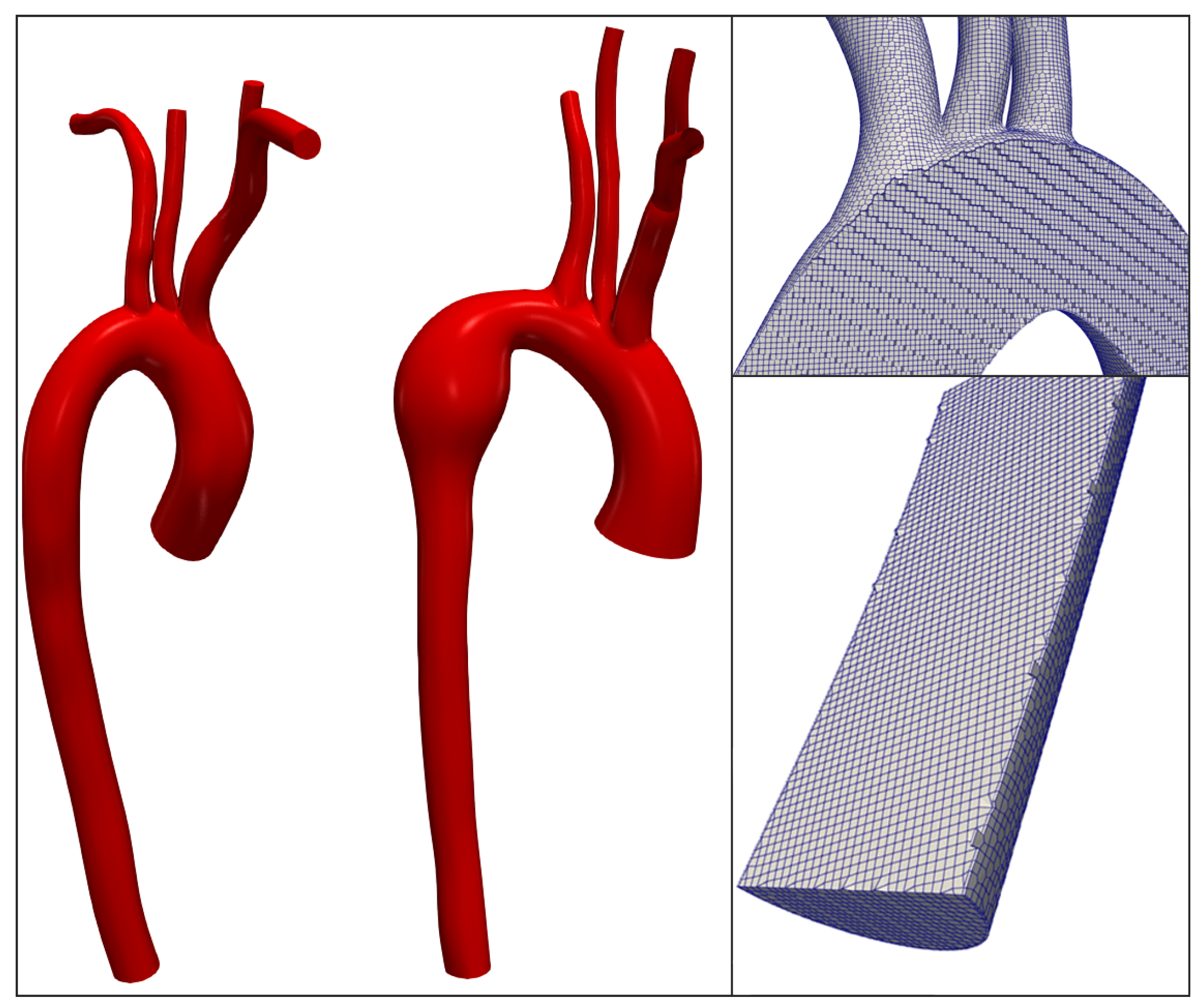
2.1. Geometries of Aorta and Generation of the Computational Domain

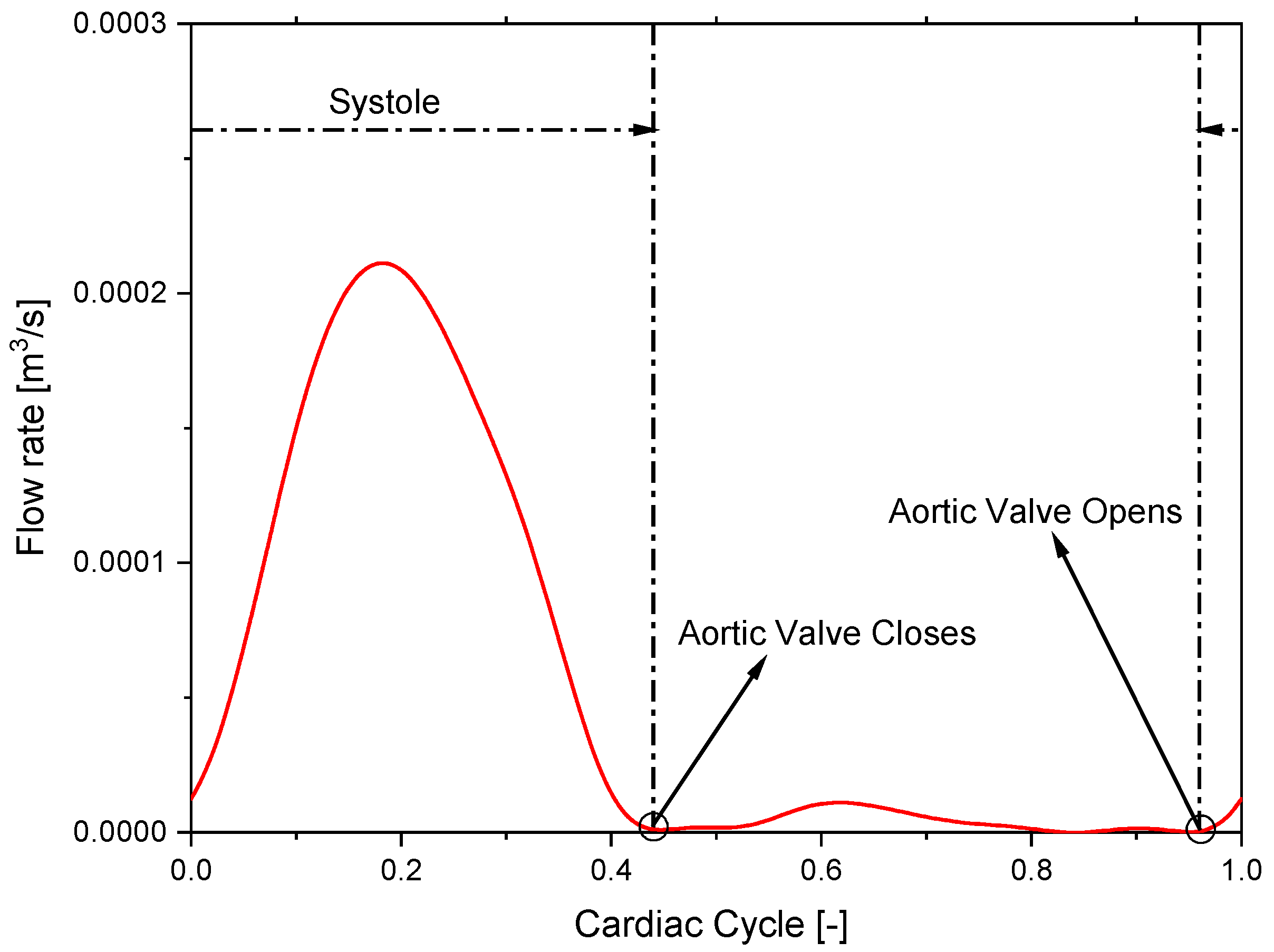
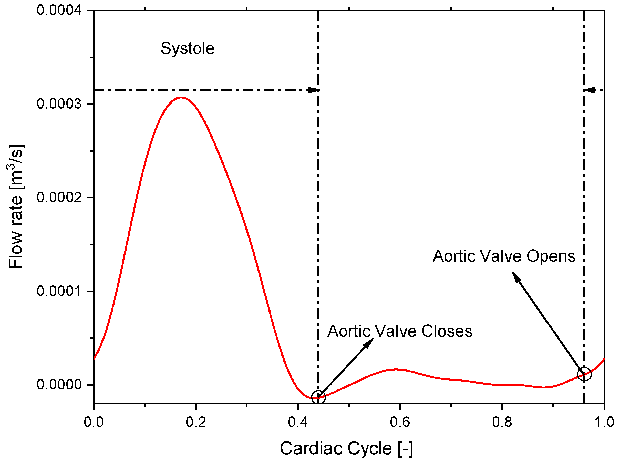
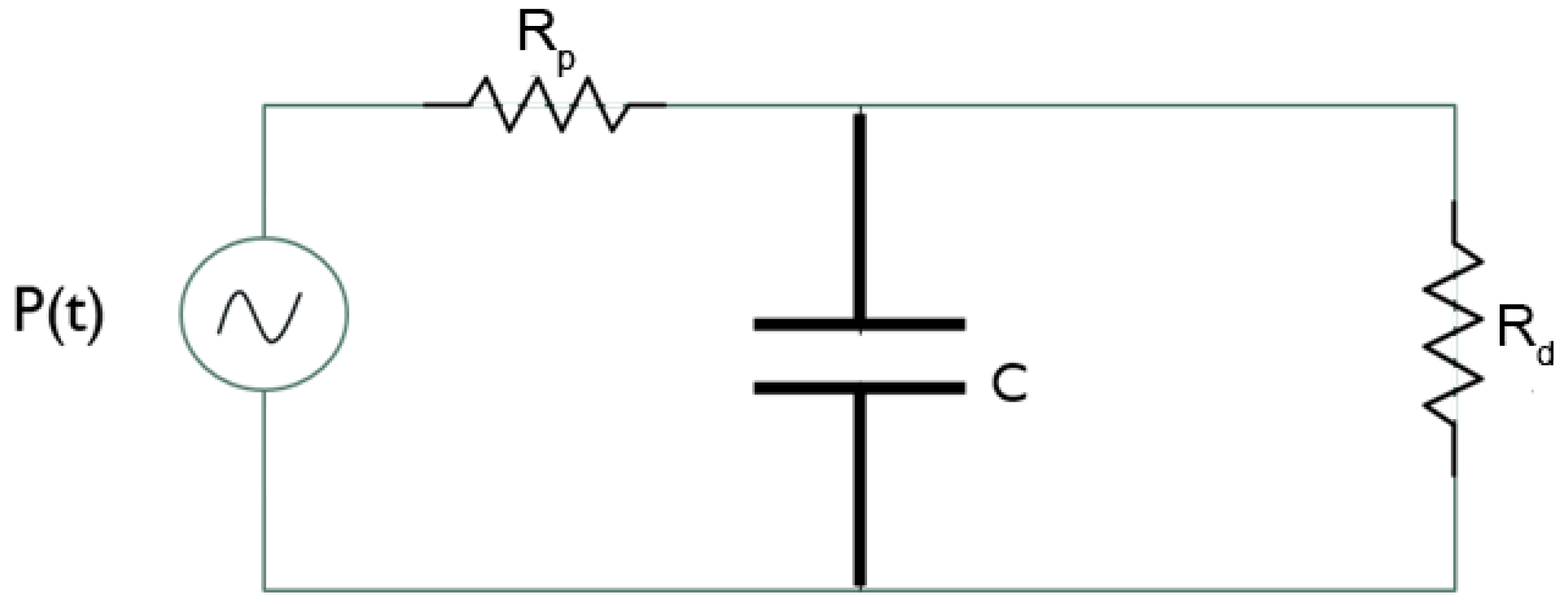
The aorta of two young male subjects of comparable age (18 and 23 years old) were considered in this study. The two geometries regard a sane and a diseased aorta. The latter presents an aneurysm on the descending section due to Marfan syndrome. Marfan syndrome is a genetic disorder that affects the body’s connective tissue. Connective tissue provides support and strength to various structures in the body, including bones, joints, ligaments, blood vessels and the heart. This condition is named after Antoine Marfan, the French paediatrician who first described it in the late 19th century. Among cardiovascular issues, Marfan syndrome affects the heart and the blood vessels, originating aortic aneurysms (bulging of the aorta) and mitral valve prolapse.

Computed tomography (CT) scans of the aorta were used to create the 3D patient-specific anatomical models used in computational fluid dynamics (CFD) simulations. All the required data were obtained from the public repository of the National Institutes of Health [17].

The aorta geometries were discretised using OpenFOAM’s utility snappyHexMesh. The computational grid so obtained was further refined and improved, creating boundary layer cells. This process refines the mesh near the boundaries, adding additional layers of hexahedral cells aligned to the boundary surface and removing irregular cells.

Three different meshes were computed to perform grid sensitivity analysis: a fine grid featuring elements of 0.5 mm average dimension, an intermediate grid of 1 mm and a coarse grid of 2 mm.

Figure 1 shows the computational grid.

For the finer grid, the boundary layer cells are 0.15 mm high. A posteriori check, using the average wall shear stress, showed that the y+ was everywhere lower than 1.

2.2. Model Setup

Governing equations of the blood flow within the aorta are essentially the continuity and the Navier–Stokes equations that express mass and momentum conservation of an incompressible flow. This assumption was deemed true considering the blood density and low velocities typical of this kind of flow [18,19].

$$\nabla ·\mathbf{u}=0$$

(1)

$$\rho \frac{D\mathbf{u}}{Dt}=-\nabla p+\rho \mathbf{f}+\mu {\nabla }^2\mathbf{u}$$

(2)

This is a system of four partial differential equations. The analytical solution of them is possible only in very few cases. A numerical solution is required due to the aorta’s complex geometry and unsteadiness of the blood flow. The equations were discretised by adopting the upwind scheme, while temporal integration was performed with the Euler method. The PIMPLE algorithm, featuring an implicit solution of the pressure–velocity coupling, was adopted to compute the solution [20,21,22,23].

A variable time step was chosen to keep the Courant number equal to 0.8.

The aorta walls are considered solid, rigid and impermeable boundaries. The blood flow near the wall was assumed to have zero velocity (no-slip boundary condition). Typically, blood exhibits non-Newtonian behaviour due to its complex composition and interactions between its components. However, it can be considered Newtonian when the shear rate exceeds 100 s${}^{-1}$ [24]. This happens particularly in large vessels such as the aorta [25]. Numerous literature studies adopted Newtonian behaviour for blood in large arteries [26,27,28]. In this particular study, the focus is on the aorta and its three major branches, where the diameters are larger than 0.1 mm. As a result, the shear rate in these large arteries is well above 100 s${}^{-1}$, allowing for the acceptance of blood as a Newtonian fluid, so a constant kinematic viscosity of $4\times {10}^{-6}$ m${}^2$/s and a density of 1050 kg/m${}^3$ were considered [29,30,31].

Based on the nominal diameter of the aorta, the peak pulsatile flow resulted in a Reynolds number ranging from 5000 to 6000, indicating turbulent flow conditions [18,32]. The Spalart–Allmaras detached eddy simulation (DES) [33,34] was chosen to model this turbulent flow. This hybrid model switches between a pure LES approach in the core turbulent region, where large unsteady turbulence scales can be resolved by grid size, and a RANS Spalart–Allmaras model near solid walls, where the typical length scale of the turbulent eddies is significantly smaller than the grid dimensions.

In the study of blood flow in the arteries, boundary conditions play a critical role in accurately representing the complex nature of the flow. At the upstream side of the artery of interest, a velocity boundary condition was prescribed.

Figure 2 and Figure 3 report the flow-rate waveforms used for the present study regarding the sane and diseased patients obtained from specific measurements [17].

A three-element Windkessel model was adopted as boundary condition for the outflow patches. The Windkessel model is a simplified model that considers the downstream arterial system as a combination of a capacitance vessel (arterial compliance) and a resistance vessel (arterial resistance). The compliance of the arteries allows them to stretch during systole, when blood is ejected from the heart, and to store part of the energy. During diastole, when the heart is relaxed, the stored energy is released, helping to maintain blood flow and pressure in the arteries. The three-element Windkessel model features a resistor to account for the resistance to blood flow caused by the aortic valve and a parallel combination of another resistor and a capacitor representing the total arterial compliance and peripheral resistance. Exploiting an electrical analogy, the three-element Windkessel model is represented in Figure 4.

The dynamics of this circuit can be mathematically expressed by the following Equation (3):

$$\left(1+\frac{R_d}{R_p}\right)Q\left(t\right)+C{R}_d\frac{dQ\left(t\right)}{dt}=\frac{P\left(t\right)}{R_p}+C\frac{dP\left(t\right)}{dt}$$

(3)

A new OpenFOAM solver called pimpleWKFoam was developed to include the three-element Windkessel model as a pressure boundary condition. Further details regarding the solution procedure are not reported here for the sake of brevity and can be found in the literature [15].

The numerical values of $R_p$, $R_d$ and C can be defined relying on specific patient measurements regarding mainly cardiac output and mean aortic pressure [16,35,36,37]. Following the various literature references, the proximal resistance results to be 10% of the overall vascular resistance while the distal resistance is 90% [38].

All the values adopted are reported in

Table 1. Resistance and compliance values for healthy aorta. LCCA = left common carotid artery; LSA = left subclavian artery; RCCA = right common carotid artery; RSA = right subclavian artery.

	${\mathit{R}}_{\mathit{p}}$ [Pa · s/m${}^5$]	${\mathit{R}}_{\mathit{d}}$ [Pa · s/m${}^5$]	C [m${}^5$/Pa]
OUTFLOW	$4.09\times {10}^7$	$1.29\times {10}^8$	$1.29\times {10}^{-8}$
LCCA	$3.23\times {10}^8$	$1.02\times {10}^9$	$1.64\times {10}^{-9}$
LSA	$2.72\times {10}^8$	$8.58\times {10}^8$	$1.94\times {10}^{-9}$
RCCA	$2.81\times {10}^8$	$8.86\times {10}^8$	$1.88\times {10}^{-9}$
RSA	$1.52\times {10}^8$	$4.80\times {10}^8$	$3.46\times {10}^{-9}$

and

Table 2. Resistance and compliance values for aneurysmatic aorta. LCCA = left common carotid artery; LSA = left subclavian artery; RCCA = right common carotid artery; RSA = right subclavian artery.

	${\mathit{R}}_{\mathit{p}}$ [Pa · s/m${}^5$]	${\mathit{R}}_{\mathit{d}}$ [Pa · s/m${}^5$]	C [m${}^5$/Pa]
OUTFLOW	$3.03\times {10}^7$	$9.13\times {10}^7$	$1.74\times {10}^{-8}$
LCCA	$2.18\times {10}^8$	$6.58\times {10}^8$	$2.42\times {10}^{-9}$
LSA	$1.74\times {10}^8$	$5.24\times {10}^8$	$3.04\times {10}^{-9}$
RCCA	$1.71\times {10}^8$	$5.14\times {10}^8$	$3.09\times {10}^{-9}$
RSA	$1.32\times {10}^8$	$3.98\times {10}^8$	$4.00\times {10}^{-9}$

.

3. Results

3.1. Convergence and Grid Sensibility Study: Preliminary Discussion

The assessment of the simulations’ accuracy and stability is crucial to ensure reliable results.

Figure 5 reports the pressure and the velocity sampled along the aorta path line, together with the computed uncertainty during the systolic peak.

The uncertainty of the numerical results was evaluated in accordance with the criterion illustrated by Roache in [20,39], where the assessment procedures adopted by the AIAA, ITTC and IEEE are described and discussed in detail.

Table 3. Grid convergence index and the order of convergence for the pressure and velocity fields.

	Grid Convergence Index	Order of Convergence
U	0.72%	2.03
p	0.23%	2.83

reports the grid convergence index and the order of convergence for the average value of pressure and velocity fields sampled along the aorta path-line.

To verify the adequacy of the adopted grid far from the aorta surfaces, where the turbulence model reduces to a large-eddy simulation, the modelled kinetic energy was evaluated and compared with the total energy. To do that, we followed Di Mascio et al. [40]. Figure 6 shows the ratio between the modelled kinetic energy and the total kinetic energy on various cross-sections of the aorta geometry for a specific temporal instant (during the systolic phase).

The modelled kinetic energy is reasonably small in the bulk flow compared to the resolved one; the ratio between the modelled and total kinetic energy is almost everywhere smaller than the value of 0.3, and therefore, the grid can be considered adequate for LES resolution, according to the Pope criterion [41] (there are only a few spots where the latter exceeds 0.3). Of course, the ratio becomes larger than 0.3 in the boundary layer on the aorta walls, where we have a Reynolds-averaged Navier–Stokes equation simulation.

Figure 7 shows a 3D volumetric representation of the velocity field captured during early, peak and late systole, 0.08, 0.18 and 0.3 s, respectively.

Unfortunately, flow measurements regarding the specific aorta here numerically investigated are not available, but the magnitude of the velocities predicted by CFD simulations are physiologically reasonable, being totally comparable with the ones measured with 4D magnetic resonance imaging (4D-MRI) in various literature works [7,42].

The same can be stated for pressure. The pressure field is reported in Figure 8, where the colour map shows the relative pressure computed with respect to a reference point chosen at the sino-tubular junction (inlet patch).

The range of variation is of the order of some hundreds of Pa, or, in mmHg, from approximately −10 mmHg to +1/+2 mmHg as usually experimentally measured with diagnostic techniques [9,43]. The pressure peak zone travels from the ascending to the descending as moving from the early to late systole phases.

3.2. Discussion of Aneurysmatic and Sane Aorta Results

Once having assessed the reliability of the computational methodology developed, further simulations regarding the aorta with the aneurysm were performed, and the results here were reported.

Figure 9 shows the velocity streamline of the sane and aneurysmatic aorta.

The flow in the normal aorta model appears to be highly stable with smooth and continuous streamlines. In contrast, in the aneurysmatic aorta model, the flow is unstable and recirculation regions are observed within the aneurysm region.

Figure 10 highlights this fact, reporting the vorticity vector. It is the curl of the velocity field. It is fundamental in understanding the behaviour of turbulent flows and the vortex formation describing the local rotation or swirling motion of fluid particles.

Observing the descending aorta, it can be noted how the flow is well organised and almost laminar, while the aneurysm enlargement creates chaotic vortical structures. The flow becomes unorganised, and the recirculation causes the blood particles to remain in prolonged contact with the aneurysm lumen surface, which can lead to the deposition of platelets on the surface [44]. The deposition of platelets on the lumen surface contributes to thrombus formation.

Figure 11 depicts the relative pressure distribution at the systole peak.

Similar pressure values were obtained for the two aorta models.

The maximum pressure is located at the aortic arch. Then, in the descending region of the aorta, the values decrease. The overall pressure variation is greater for the aneurysmatic aorta as a consequence of the structure of the flow field [45]. The aneurysm cavity presents a low-pressure region. A pressure minimum can be observed at the centre of the vortex as a consequence of the turbulent energy here dissipated.

The distribution of wall shear stress (WSS) on the artery walls is an important parameter that can be used to investigate risks related to the aneurysms of the aortic arch [45,46]. Abnormal low and high WSS patterns can have significant implications for the development of vascular diseases on the artery walls. The advantage of CFD simulations in studying aortic flow is that they can help identify regions with abnormal WSS levels, which may be more prone to dilatation or aneurysm formation.

Figure 12 reports the WSS at the peak systole for both the aorta.

The aneurysm zone and the region where the aorta branches off in arteries are subject to more intensity compared to the normal aorta’s relative areas. The descending section of the diseased aorta, downstream of the enlargement, also presents spots of high WSS. The differences in WSS values between subjects with aneurysms and normal subjects can be attributed to many factors. However, among them, the variation of the velocity field should be cited as a consequence of the distorted aorta geometry.

4. Conclusions

This study aims to contribute to the understanding of thoracic aortic flow characteristics. CFD simulations were performed using real-patient flow characteristics for both a normal subject and a subject with an aneurysm of the thoracic aorta. Real 3D geometries of the aorta were exploited with patient-specific pulsatile waveform used as the inlet boundary condition to reflect the real cardiac cycle. A three-element Windkessel lumped parameter model was implemented in a new OpenFOAM solver called pimpleWKFoam to set the pressure outlet boundary conditions properly. The main findings are:

• The developed methodology with the implementation of the WK model is capable of reproducing the fluid-dynamic characteristics of the aortic flow, providing realistic pressure and velocity field values.
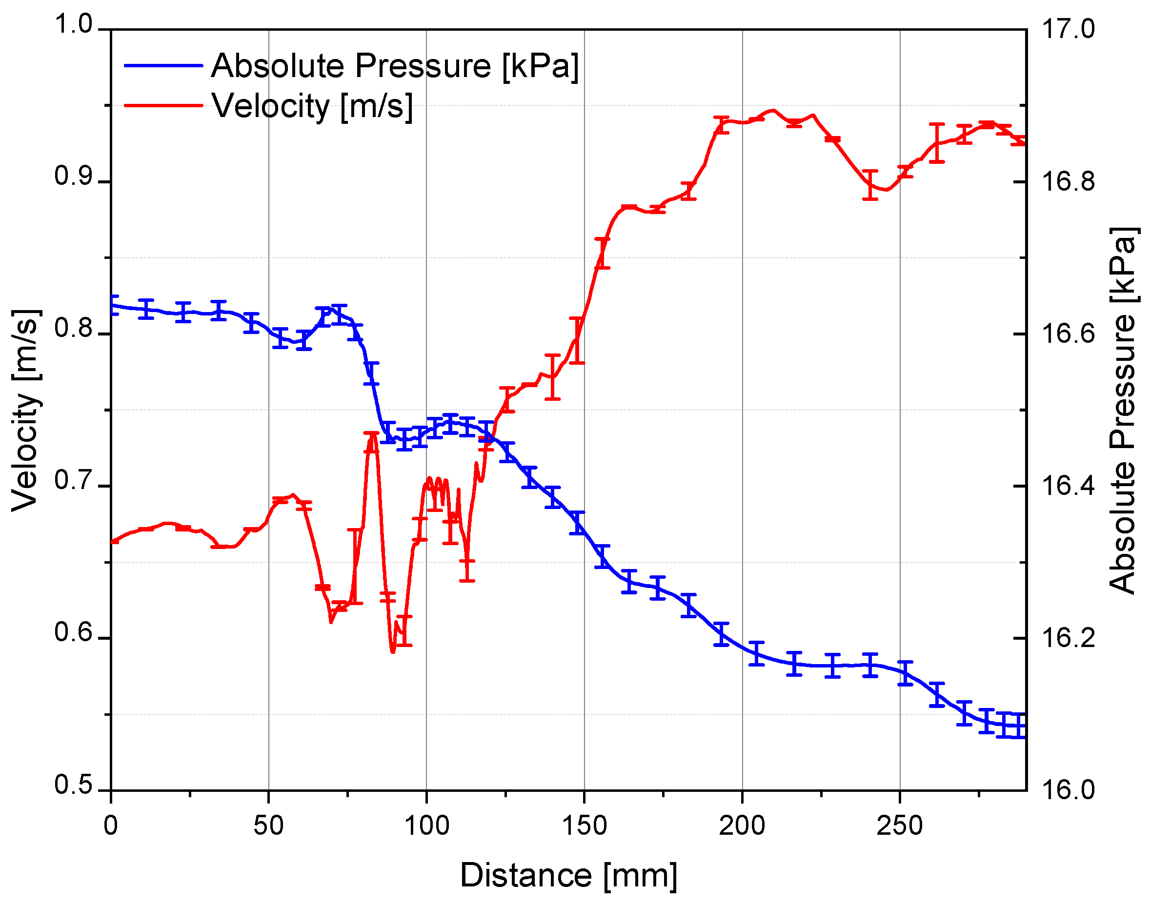
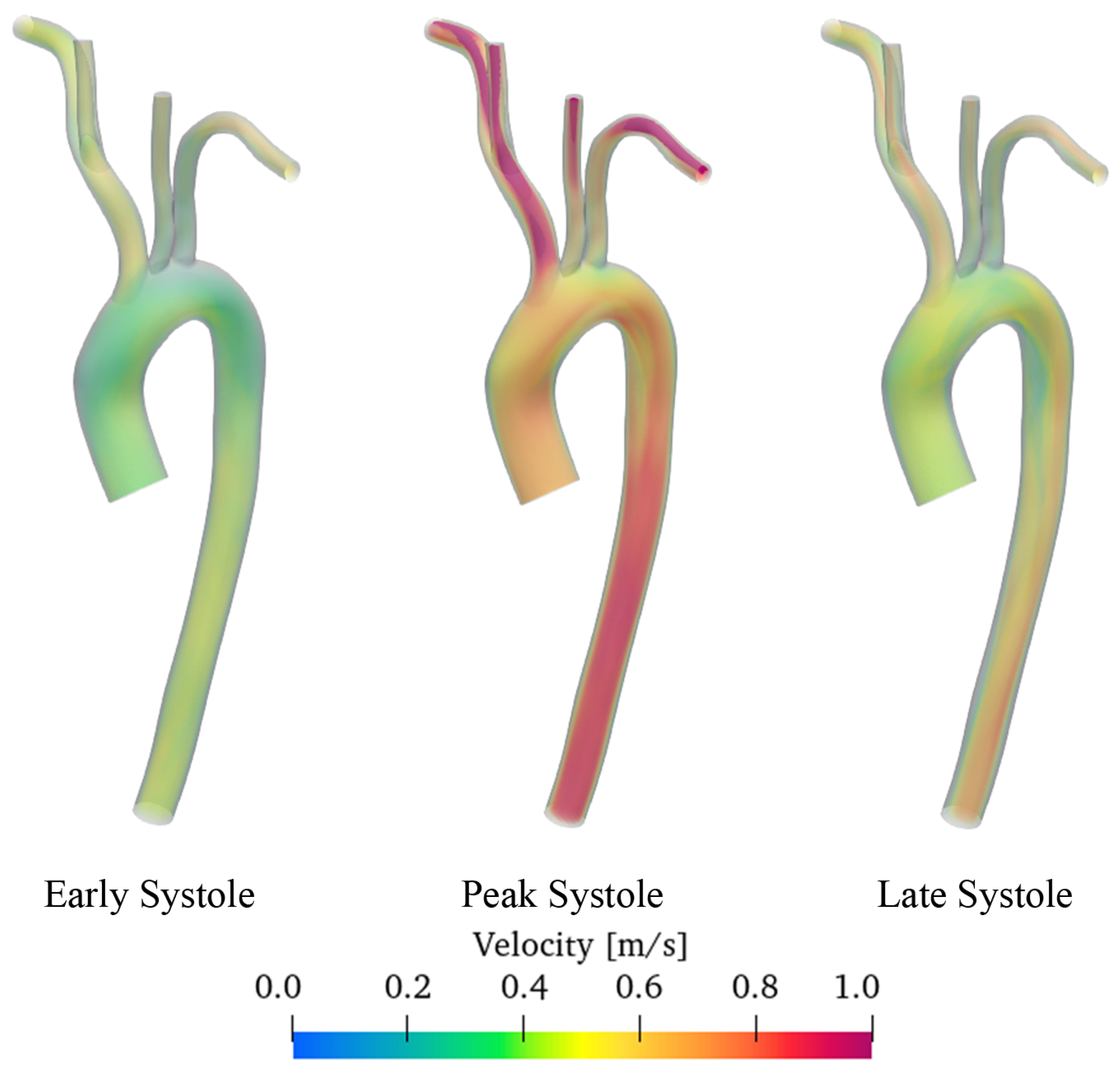
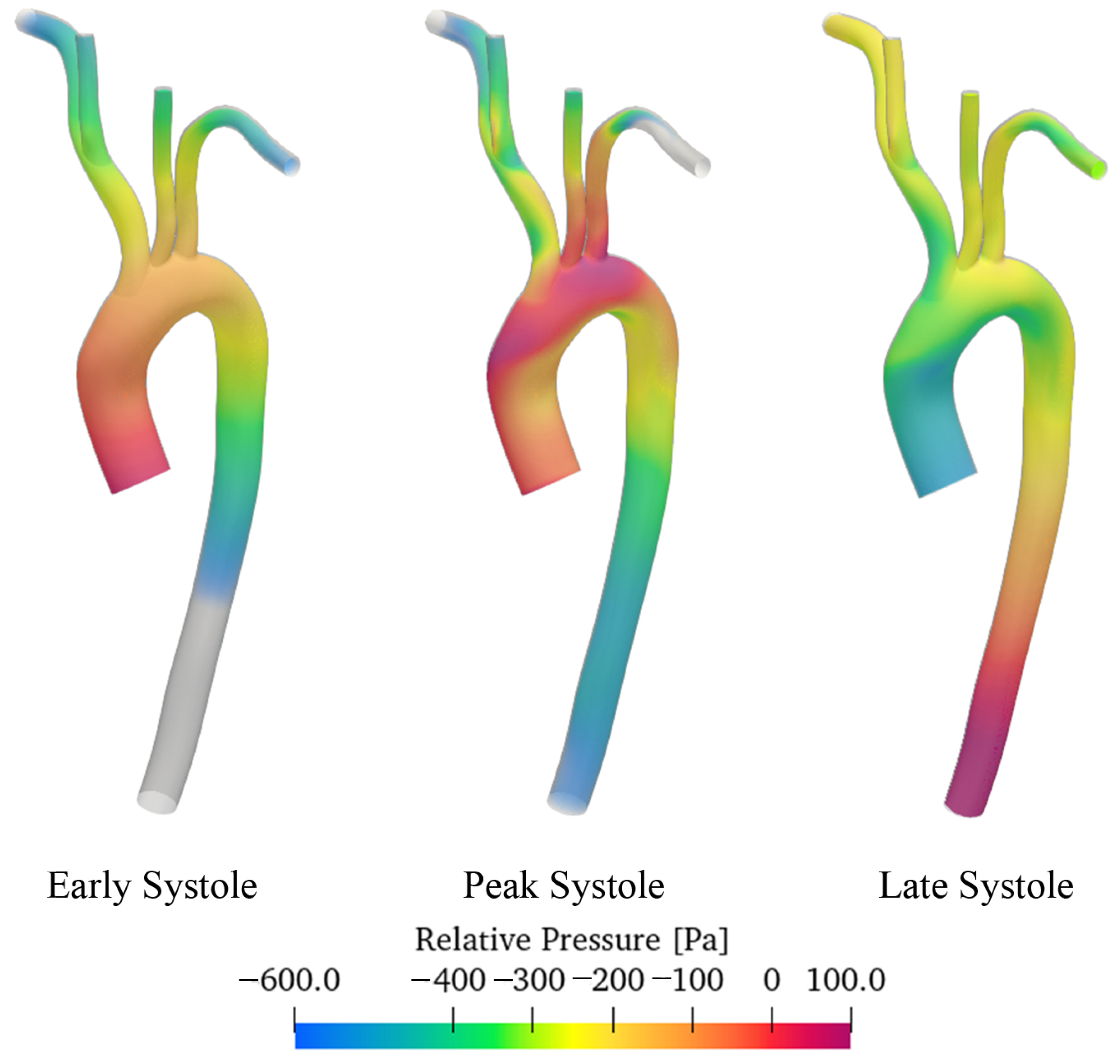
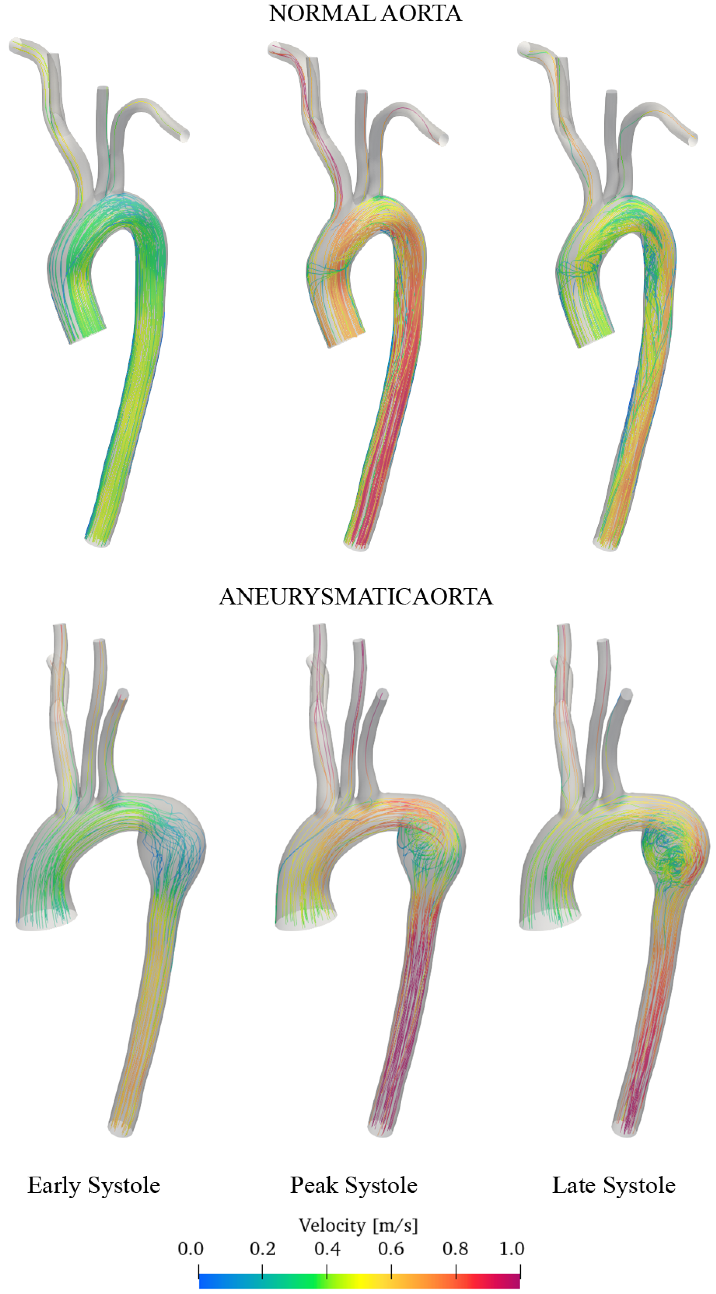
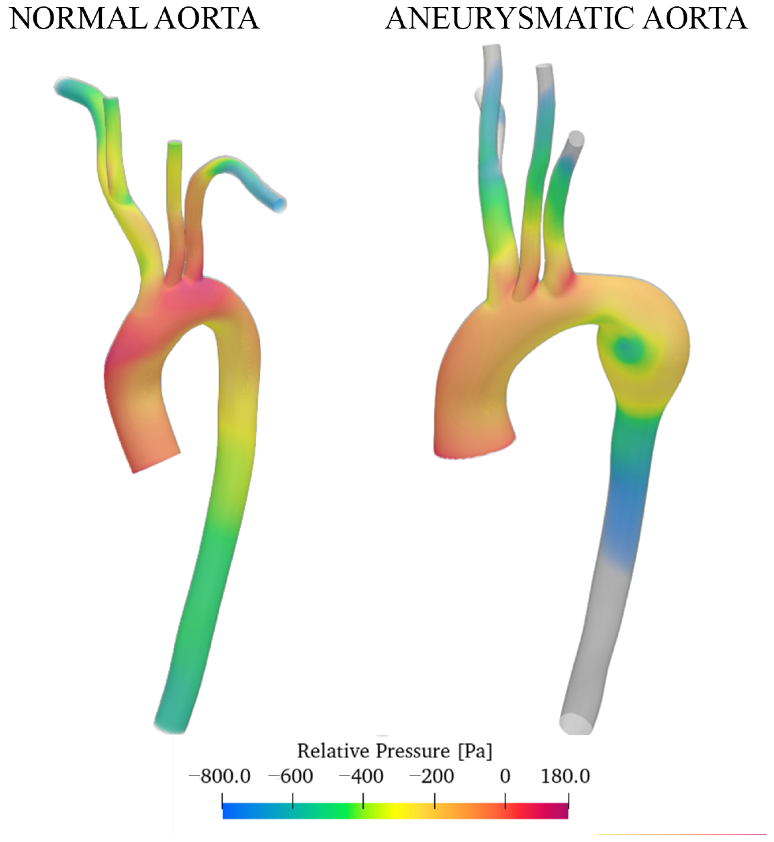
• In the thoracic aorta, blood velocity is on the order of 1 m/s, while the pressure varies by about 500/700 Pa crossing the aorta itself.
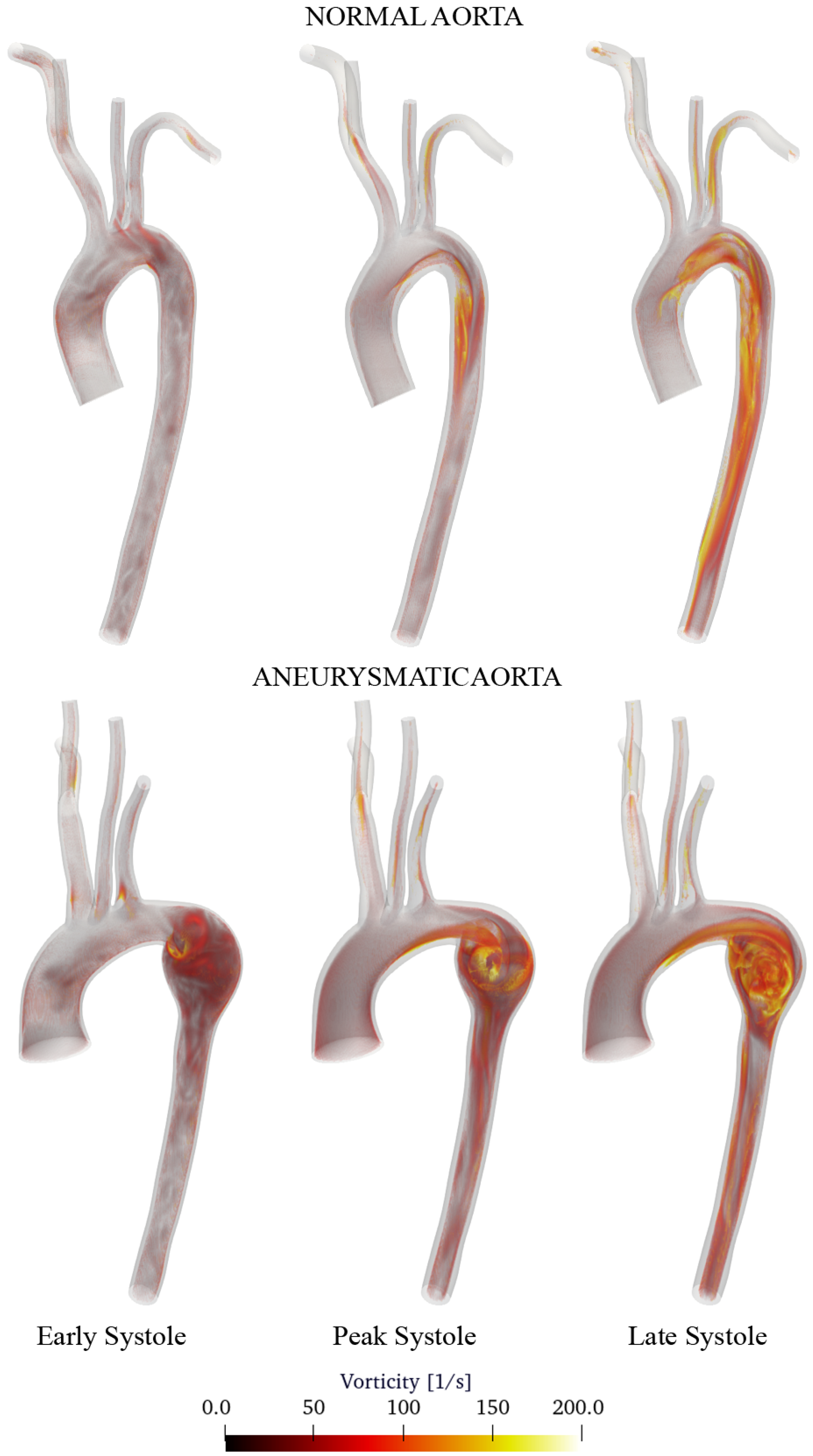
• Aneurysm onset causes the flow field to become unstable, and recirculation zones grow in the enlargement section with the consequent deposition of platelets and thrombus formation.
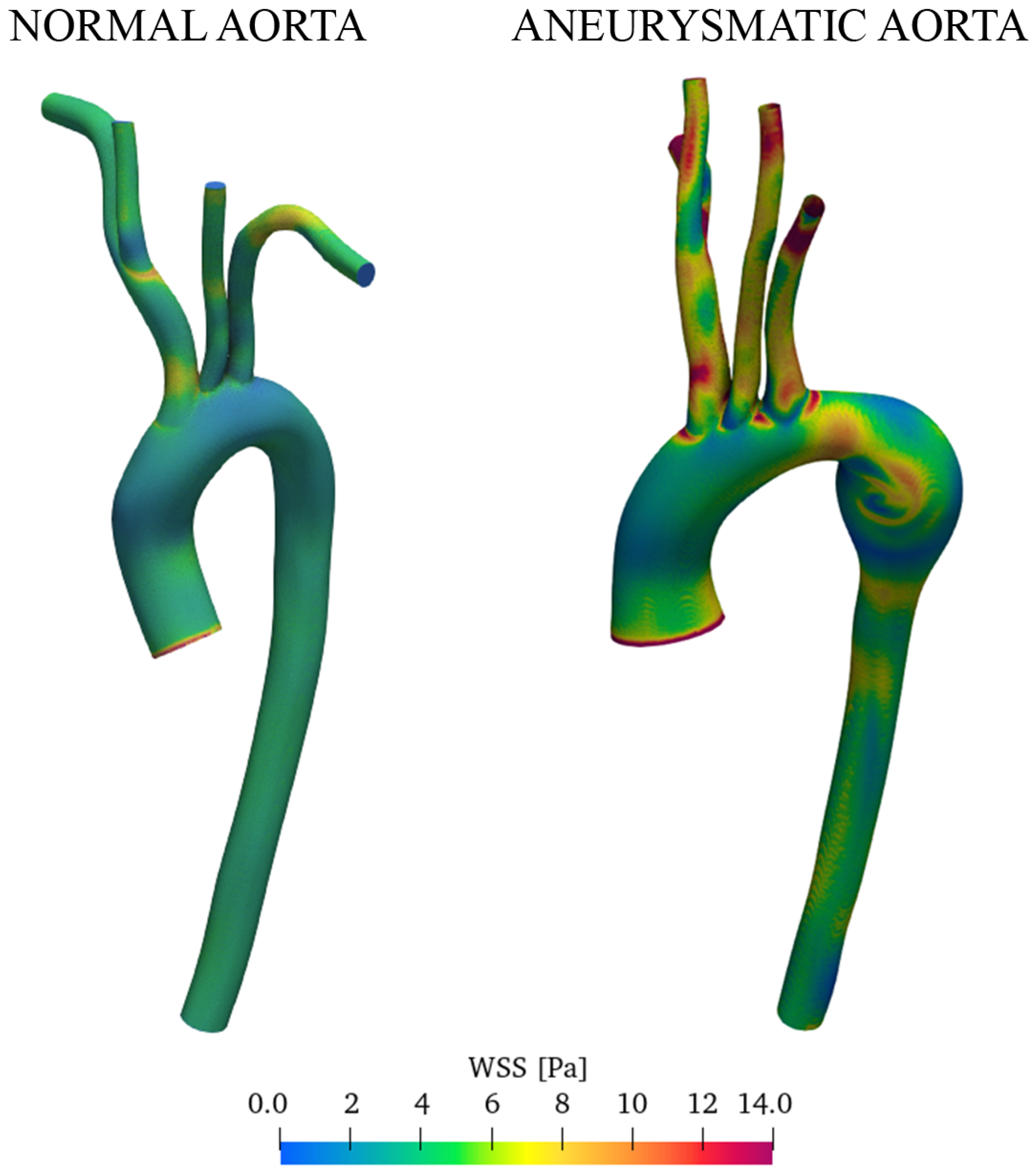
• CFD simulations allow identifying regions with WSS levels that may be more prone to dilatation or aneurysm formation. The magnitude of the WSS reaches the maximum values in the enlarged zone.

Future developments of this work will regard the implementation of elastic walls with a fluid-structure-interaction (FSI) model.

References

1. Gaidai, O.; Cao, Y.; Loginov, S. Global Cardiovascular Diseases Death Rate Prediction. Curr. Probl. Cardiol. 2023, 48, 101622. [Google Scholar] [CrossRef] [PubMed]
2. Nerem, R. Hot film measurement of arterial blood flow and observation of flow disturbances. In Cardiovascular Flow Dynamics and Measurement; University Park Press: University Park, PA, USA, 1977; pp. 191–215. [Google Scholar]
3. Smedby, Ö. Geometric risk factors for atherosclerosis in the aortic bifurcation: A digitized angiography study. Ann. Biomed. Eng. 1996, 24, 481–488. [Google Scholar] [CrossRef] [PubMed]
4. Menichini, C.; Xu, X.Y. Mathematical modeling of thrombus formation in idealized models of aortic dissection: Initial findings and potential applications. J. Math. Biol. 2016, 73, 1205–1226. [Google Scholar] [CrossRef] [PubMed]
5. Vasava, P.; Jalali, P.; Dabagh, M.; Kolari, P.J. Finite Element Modelling of Pulsatile Blood Flow in Idealized Model of Human Aortic Arch: Study of Hypotension and Hypertension. Comput. Math. Methods Med. 2012, 2012, 861837. [Google Scholar] [CrossRef] [PubMed]
6. Voges, I.; Jerosch-Herold, M.; Hedderich, J.; Pardun, E.; Hart, C.; Gabbert, D.D.; Hansen, J.H.; Petko, C.; Kramer, H.H.; Rickers, C. Normal values of aortic dimensions, distensibility, and pulse wave velocity in children and young adults: A cross-sectional study. J. Cardiovasc. Magn. Reson. 2012, 14, 77. [Google Scholar] [CrossRef] [PubMed]
7. Bouaou, K.; Bargiotas, I.; Dietenbeck, T.; Bollache, E.; Soulat, G.; Craiem, D.; Houriez-Gombaud-Saintonge, S.; De Cesare, A.; Gencer, U.; Giron, A.; et al. Analysis of aortic pressure fields from 4D flow MRI in healthy volunteers: Associations with age and left ventricular remodeling. J. Magn. Reson. Imaging 2019, 50, 982–993. [Google Scholar] [CrossRef]
8. Lamata, P.; Pitcher, A.; Krittian, S.; Nordsletten, D.; Bissell, M.M.; Cassar, T.; Barker, A.J.; Markl, M.; Neubauer, S.; Smith, N.P. Aortic relative pressure components derived from four-dimensional flow cardiovascular magnetic resonance. Magn. Reson. Med. 2014, 72, 1162–1169. [Google Scholar] [CrossRef]
9. Rengier, F.; Delles, M.; Eichhorn, J.; Azad, Y.J.; von Tengg-Kobligk, H.; Ley-Zaporozhan, J.; Dillmann, R.; Kauczor, H.U.; Unterhinninghofen, R.; Ley, S. Noninvasive 4D pressure difference mapping derived from 4D flow MRI in patients with repaired aortic coarctation: Comparison with young healthy volunteers. Int. J. Cardiovasc. Imaging 2015, 31, 823–830. [Google Scholar] [CrossRef]
10. Yull Park, J.; Young Park, C.; Mo Hwang, C.; Sun, K.; Goo Min, B. Pseudo-organ boundary conditions applied to a computational fluid dynamics model of the human aorta. Comput. Biol. Med. 2007, 37, 1063–1072. [Google Scholar] [CrossRef]
11. Madhavan, S.; Kemmerling, E.M.C. The effect of inlet and outlet boundary conditions in image-based CFD modeling of aortic flow. Biomed. Eng. Online 2018, 17, 66. [Google Scholar] [CrossRef]
12. Pirola, S.; Cheng, Z.; Jarral, O.; O’Regan, D.; Pepper, J.; Athanasiou, T.; Xu, X. On the choice of outlet boundary conditions for patient-specific analysis of aortic flow using computational fluid dynamics. J. Biomech. 2017, 60, 15–21. [Google Scholar] [CrossRef] [PubMed]
13. Hardman, D.; Semple, S.I.; Richards, J.M.; Hoskins, P.R. Comparison of patient-specific inlet boundary conditions in the numerical modelling of blood flow in abdominal aortic aneurysm disease. Int. J. Numer. Methods Biomed. Eng. 2013, 29, 165–178. [Google Scholar] [CrossRef] [PubMed]
14. Antonuccio, M.N.; Mariotti, A.; Fanni, B.M.; Capellini, K.; Capelli, C.; Sauvage, E.; Celi, S. Effects of Uncertainty of Outlet Boundary Conditions in a Patient-Specific Case of Aortic Coarctation. Ann. Biomed. Eng. 2021, 49, 3494–3507. [Google Scholar] [CrossRef]
15. Catanho, M.; Sinha, M.; Vijayan, V. Model of Aortic Blood Flow Using the Windkessel Effect; University of California of San Diego: San Diego, CA, USA, 2012. [Google Scholar]
16. Westerhof, N.; Lankhaar, J.W.; Westerhof, B.E. The arterial Windkessel. Med Biol. Eng. Comput. 2009, 47, 131–141. [Google Scholar] [CrossRef] [PubMed]
17. Wilson, N.M.; Ortiz, A.K.; Johnson, A.B. The Vascular Model Repository: A Public Resource of Medical Imaging Data and Blood Flow Simulation Results. J. Med. Device 2013, 7, 0409231. [Google Scholar] [CrossRef] [PubMed]
18. Caballero, A.D.; Laín, S. A Review on Computational Fluid Dynamics Modelling in Human Thoracic Aorta. Cardiovasc. Eng. Technol. 2013, 4, 103–130. [Google Scholar] [CrossRef]
19. Etli, M.; Canbolat, G.; Karahan, O.; Koru, M. Numerical investigation of patient-specific thoracic aortic aneurysms and comparison with normal subject via computational fluid dynamics (CFD). Med. Biol. Eng. Comput. 2021, 59, 71–84. [Google Scholar] [CrossRef]
20. Duronio, F.; Di Mascio, A.; De Vita, A.; Innocenzi, V.; Prisciandaro, M. Eulerian–Lagrangian modeling of phase transition for application to cavitation-driven chemical processes. Phys. Fluids 2023, 35, 053305. [Google Scholar] [CrossRef]
21. Dutta, H. Mathematical Methods in Engineering and Applied Sciences; Mathematics and Its Applications; CRC Press: Boca Raton, FL, USA, 2020. [Google Scholar]
22. De Vita, M.; Duronio, F.; De Vita, A.; De Berardinis, P. Adaptive Retrofit for Adaptive Reuse: Converting an Industrial Chimney into a Ventilation Duct to Improve Internal Comfort in a Historic Environment. Sustainability 2022, 14, 3360. [Google Scholar] [CrossRef]
23. Duronio, F.; Mascio, A.D.; Villante, C.; Anatone, M.; Vita, A.D. ECN Spray G: Coupled Eulerian internal nozzle flow and Lagrangian spray simulation in flash boiling conditions. Int. J. Engine Res. 2023, 24, 1530–1544. [Google Scholar] [CrossRef]
24. Berger, S.A.; Jou, L.D. Flows in Stenotic Vessels. Annu. Rev. Fluid Mech. 2000, 32, 347–382. [Google Scholar] [CrossRef]
25. Pedley, T.J. The Fluid Mechanics of Large Blood Vessels; Cambridge University Press: Cambridge, UK, 1980. [Google Scholar] [CrossRef]
26. Morris, L.; Delassus, P.; Callanan, A.; Walsh, M.; Wallis, F.; Grace, P.; McGloughlin, T. 3-D Numerical Simulation of Blood Flow through Models of the Human Aorta. J. Biomech. Eng. 2005, 127, 767–775. [Google Scholar] [CrossRef] [PubMed]
27. Youssefi, P.; Gomez, A.; Arthurs, C.; Sharma, R.; Jahangiri, M.; Alberto Figueroa, C. Impact of Patient-Specific Inflow Velocity Profile on Hemodynamics of the Thoracic Aorta. J. Biomech. Eng. 2017, 140, 011002. [Google Scholar] [CrossRef]
28. Qian, Y.; Liu, J.L.; Itatani, K.; Miyaji, K.; Umezu, M. Computational Hemodynamic Analysis in Congenital Heart Disease: Simulation of the Norwood Procedure. Ann. Biomed. Eng. 2010, 38, 2302–2313. [Google Scholar] [CrossRef] [PubMed]
29. Zakaria, M.S.; Ismail, F.; Tamagawa, M.; Abdul Azi, A.F.; Wiriadidjaya, S.; Basri, A.A.; Ahmad, K.A. Computational Fluid Dynamics Study of Blood Flow in Aorta using OpenFOAM. J. Adv. Res. Fluid Mech. Therm. Sci. 2020, 43, 81–89. [Google Scholar]
30. Boyd, J.; Buick, J.M. Comparison of Newtonian and non-Newtonian flows in a two-dimensional carotid artery model using the lattice Boltzmann method. Phys. Med. Biol. 2007, 52, 6215. [Google Scholar] [CrossRef]
31. Otani, T.; Nakamura, M.; Fujinaka, T.; Hirata, M.; Kuroda, J.; Shibano, K.; Wada, S. Computational fluid dynamics of blood flow in coil-embolized aneurysms: Effect of packing density on flow stagnation in an idealized geometry. Med. Biol. Eng. Comput. 2013, 51, 901–910. [Google Scholar] [CrossRef]
32. Antón, R.; Chen, C.Y.; Hung, M.Y.; Finol, E.; Pekkan, K. Experimental and computational investigation of the patient-specific abdominal aortic aneurysm pressure field. Comput. Methods Biomech. Biomed. Eng. 2015, 18, 981–992. [Google Scholar] [CrossRef]
33. Spalart, P.R.; Deck, S.; Shur, M.L.; Squires, K.D.; Strelets, M.K.; Travin, A. A new version of detached-eddy simulation, resistant to ambiguous grid densities. Theor. Comput. Fluid Dyn. 2006, 20, 181–195. [Google Scholar] [CrossRef]
34. Di Angelo, L.; Duronio, F.; De Vita, A.; Di Mascio, A. Cartesian Mesh Generation with Local Refinement for Immersed Boundary Approaches. J. Mar. Sci. Eng. 2021, 9, 572. [Google Scholar] [CrossRef]
35. Safar, M.E.; Lévy, B.I. Chapter 13—Resistance Vessels in Hypertension. In Comprehensive Hypertension; Lip, G.Y., Hall, J.E., Eds.; Mosby: Philadelphia, PA, USA, 2007; pp. 145–150. [Google Scholar] [CrossRef]
36. Pochet, T.; Gerard, P.; Marnette, J.M.; D’orio, V.; Marcelle, R.; Fatemi, M.; Fossion, A.; Juchmes, J. Identification of three-element windkessel model: Comparison of time and frequency domain techniques. Arch. Int. Physiol. Biochim. Biophys. 1992, 100, 295–301. [Google Scholar] [CrossRef] [PubMed]
37. Tricarico, R.; Berceli, S.A.; Tran-Son-Tay, R.; He, Y. Non-invasive estimation of the parameters of a three-element windkessel model of aortic arch arteries in patients undergoing thoracic endovascular aortic repair. Front. Bioeng. Biotechnol. 2023, 11, 1127855. [Google Scholar] [CrossRef] [PubMed]
38. Lungu, A.; Wild, J.; Capener, D.; Kiely, D.; Swift, A.; Hose, D. MRI model-based non-invasive differential diagnosis in pulmonary hypertension. J. Biomech. 2014, 47, 2941–2947. [Google Scholar] [CrossRef]
39. Roache, P.J. Quantification of uncertainty in computational fluid dynamics. Annu. Rev. Fluid Mech. 1997, 29, 123–160. [Google Scholar] [CrossRef]
40. Di Mascio, A.; Dubbioso, G.; Muscari, R. Vortex structures in the wake of a marine propeller operating close to a free surface. J. Fluid Mech. 2022, 949, A33. [Google Scholar] [CrossRef]
41. Pope, S.B.; Pope, S.B. Turbulent Flows; Cambridge University Press: Cambridge, UK, 2000. [Google Scholar]
42. Garcia, J.; Barker, A.J.; Markl, M. The Role of Imaging of Flow Patterns by 4D Flow MRI in Aortic Stenosis. JACC Cardiovasc. Imaging 2019, 12, 252–266. [Google Scholar] [CrossRef]
43. Soulat, G.; McCarthy, P.; Markl, M. 4D Flow with MRI. Annu. Rev. Biomed. Eng. 2020, 22, 103–126. [Google Scholar] [CrossRef]
44. Bluestein, D.; Niu, L.; Schoephoerster, R.T.; Dewanjee, M.K. Steady Flow in an Aneurysm Model: Correlation Between Fluid Dynamics and Blood Platelet Deposition. J. Biomech. Eng. 1996, 118, 280–286. [Google Scholar] [CrossRef]
45. Vinoth, R.; Kumar, D.; Adhikari, R.; Vijayapradeep, S.; Geetha, K.; Ilavarasi, R.; Mahalingam, S. Steady and Transient Flow CFD Simulations in an Aorta Model of Normal and Aortic Aneurysm Subjects. In Proceedings of the International Conference on Sensing and Imaging; Jiang, M., Ida, N., Louis, A.K., Quinto, E.T., Eds.; Springer International Publishing: Cham, Switzerland, 2019; pp. 29–43. [Google Scholar]
46. Febina, J.; Sikkandar, M.Y.; Sudharsan, N.M. Wall Shear Stress Estimation of Thoracic Aortic Aneurysm Using Computational Fluid Dynamics. Comput. Math. Methods Med. 2018, 2018, 7126532. [Google Scholar] [CrossRef]
Figure 1. Sane and diseased aorta geometries are shown on the left while, on the right, some details of the computational grid used are shown.
Fluids 08 00272 g001
Figure 2. Pulsatile waveform used as Dirichlet inlet boundary condition for the sane patient.
Fluids 08 00272 g002
Figure 3. Pulsatile waveform used as Dirichlet inlet boundary condition for the diseased patient (aorta with aneurysm).
Fluids 08 00272 g003
Figure 4. Electrical analog of the 3-element Windkessel model.
Fluids 08 00272 g004
Figure 5. Pressure and velocity sampled on the aorta path-line during the systolic peak.
Fluids 08 00272 g005
Figure 6. K m o d / ( K m o d + K r e s ) horizontal sections.
Fluids 08 00272 g006
Figure 7. Computed velocity flow field of the sane aorta.
Fluids 08 00272 g007
Figure 8. Computed pressure field of the sane aorta.
Fluids 08 00272 g008
Figure 9. Comparison of sane and diseased aorta. Streamline coloured accordingly with the velocity magnitude.
Fluids 08 00272 g009
Figure 10. Comparison of sane and diseased aorta. 3D visualisation of the vorticity vector.
Fluids 08 00272 g010
Figure 11. Relative pressure with reference to the inlet section. Comparison of sane and aneurysmatic aorta.
Fluids 08 00272 g011
Figure 12. WSS acting on the boundary surfaces of the computational fluid domain. Comparison of sane and aneurysmatic aorta.
Fluids 08 00272 g012