Article

Image-Based Numerical Investigation in an Impending Abdominal Aneurysm Rupture

by
Maria Antonietta Boniforti
1,*,
Maria Chiara Cesaroni
1,
Roberto Magini
1,
Edoardo Pasqui
2 and
Gianmarco de Donato
2
1
Department of Civil, Building, and Environmental Engineering, Sapienza University, 00184 Rome, Italy
2
Department of Medicine, Surgery and Neuroscience, University of Siena, 53100 Siena, Italy
*
Author to whom correspondence should be addressed.
Fluids 2022, 7(8), 269; https://doi.org/10.3390/fluids7080269
Submission received: 7 July 2022 / Revised: 28 July 2022 / Accepted: 2 August 2022 / Published: 5 August 2022
(This article belongs to the Special Issue Image-Based Computational and Experimental Biomedical Flows)

Abstract

:
Blood flow dynamics plays a crucial role in the growth and rupture of abdominal aortic aneurysms. The aim of this study was to analyze the possibility of predicting aneurysmal rupture by numerical investigations based on diagnostic images. The blood flow dynamics was analyzed in a patient-specific abdominal aortic aneurysm, reconstructed from CT images of an aneurysm while it was rupturing. The patient-specific geometry was virtually repaired in order to obtain a non-ruptured model representative of the geometry immediately preceding the rupture. To reproduce physiological conditions, numerical simulations were performed under pulsatile flow conditions, and blood was modelled as a non-Newtonian fluid, using the Carreau rheological model. Hemodynamic parameters that influence the rupture of the aneurysm were investigated, and their possible association with vascular disease was discussed. The results of the numerical simulations indicated regions of slow recirculation and low values of Time Averaged Wall Shear Stress (TAWSS) in the region of rupture. Unlike literature results, a high Oscillatory Shear Index (OSI) was not clearly found in this region. Nevertheless, just in the region where the rupture will occur, high values of Endothelial Cell Activation Potential index (ECAP) were found. This index is therefore extremely significant for assessing the vulnerability of the aortic wall and locating the critical rupture region.

Graphical Abstract

1. Introduction

Abdominal aortic aneurysms (AAAs) are pathological dilatations of the abdominal aorta, which represent a life-threatening condition, as their rupture is often lethal. They involve an increase in diameter above 50% with respect to the diameter of the healthy aorta, which is about 2.0 cm in the abdomen [1,2].
Surgery is generally recommended if the maximum aortic diameter exceeds 5.0 cm in women and 5.5 cm in men, or if the maximum diameter shows a growth rate greater than 0.5–1.0 cm in one year [3,4].
Nevertheless, rupture of small and medium abdominal aortic aneurysms is found as well as perfect integrity of large AAAs over long periods [2,5,6,7,8,9,10]. Consequently, maximum AAA diameter cannot be the only indicator to predict the AAA’s rupture and plan the surgery.
A rupture potential index (RPI), defined as the ratio of the locally acting wall stress to the wall strength, was firstly proposed by Vande Geest et al., which found for ruptured aneurysm a mean RPI value equal to 0.48 [11]. This index was found to be high in ruptured aortic aneurysms. The evaluation of this index allowed a significant differentiation of the risk of rupture for diameters in the range of 55–75 mm, for which the criterion of the maximum diameter was not always useful [12]. Although this index and some others can help to predict AAA rupture risk, their validation is often difficult. Furthermore, they are often based only on mechanical quantities without considering the effect of the pulsatile flow that interacts with the arterial wall.
Actually, intraluminal thrombus (ILT) accumulation and progression of the AAA pathology determine variations in the physiological geometry of the artery, which result in a disturbed blood flow. The perturbed flow plays in turn a crucial role in the growth of the abdominal aortic aneurysm (AAAs) and contributes to the progression of the AAA pathology. In fact, it indirectly determines damage to the endothelium and increases the degeneration of the arterial wall.
As matter of fact, the biological relevance of the wall shear stress (WSS) and its relationship with the endothelium was largely emphasized [13]. Changes in magnitude and direction of the WSS vector act on blood vessels owing to the presence of the endothelial cells, which form the inner lining of the vessel walls. WSS sensed by endothelial cells plays an important role in the development, remodeling and maintenance of the vascular system [13]. Non-physiological shear stress associated with the perturbed flow in the aneurysm correlates with atherosclerotic lesion, as well documented in literature [14,15]. This non-physiologic shear stress was also indicated to promote the growth and possible rupture of the aneurysm [16].
Deterioration of the arterial wall was also associated with low Time Averaged Wall Shear Stresses (TAWSS) and recirculating blood regions [16,17,18,19]. While unidirectional wall shear stress characterizes healthy regions of the arterial wall, regions exposed to disturbed flow conditions are associated with Oscillatory Shear Stress (OSI), which induces monocyte adhesion in endothelial cells and inflammatory response [20]. In abdominal aortic aneurysms, compared to healthy aorta values, lower WSS and higher OSI have been found [18]. However, some contradictory results were found, since ILT growth was observed in regions of low OSI [21,22].
To help clinicians in the difficult decision on the need for surgery, this study highlights how some hemodynamic parameters can provide useful indications for the prediction of aneurysm rupture.
In particular, numerical simulations of the blood flow have been employed to investigate the relationship between hemodynamics and aneurysm rupture. A patient-specific model of an abdominal aortic aneurysm was reconstructed from a CT angiography of a ruptured aneurysm, obtained immediately after the rupture in the Hospital of the University of Siena (Italy). The geometry of the aneurysm immediately preceding the rupture was assumed to be similar to the ruptured geometry since it does not change significantly during the rupture. Based on this hypothesis, the patient-specific model reconstructed from the CT diagnostic images was virtually repaired, and a non-ruptured model, which was representative of the geometry immediately preceding the rupture, was used to investigate the blood flow dynamics.
Numerical simulations in physiological conditions of pulsating motion were carried out, and hemodynamic parameters that can predict possible rupture of the aneurysm were analyzed. In particular, 2D streamlines on suitable longitudinal cross-sections were studied throughout the cardiac cycle. Moreover, hemodynamic quantities that can help in identifying artery regions that could be subject to rupture, i.e., time-averaged velocity, TAWSS, OSI, and Endothelial Cell Activation Potential (ECAP), were evaluated.
This work is organized as follows. Firstly, in paragraph 2, the methods and setting up of the study are presented. In particular, the procedure for the 3D reconstruction of the pre-rupture patient-specific aneurysms from the CT images is described, and the governing equations and hypotheses for the numerical fluid dynamics model are furnished. Special attention is also paid to the fluid dynamics parameters used to describe the blood flow in the aneurysm, providing a physics-based interpretation of their role. In paragraph 3, the main results obtained from the computational investigation are presented, with the aim of a better understanding of the blood flow in the AAA’s pre-rupture condition. Finally, some concluding remarks are provided, taking into account the link between the hemodynamic fields and the presence and position of rupture regions. In particular, the important role of the ECAP index was highlighted.
It is important to underline the innovative methodology used to obtain the pre-rupture model of the aneurysm, which allows a hemodynamic investigation in an unruptured aneurysm in impending rupture, with the advantage of knowing the real future position of the rupture region.
The results of this work highlight the importance of a patient-specific fluid dynamics investigation to predict a possible rupture of the aneurysm and to aid clinicians in the difficult decision regarding the need for surgery.

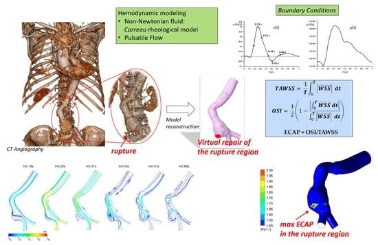
2. Materials and Methods

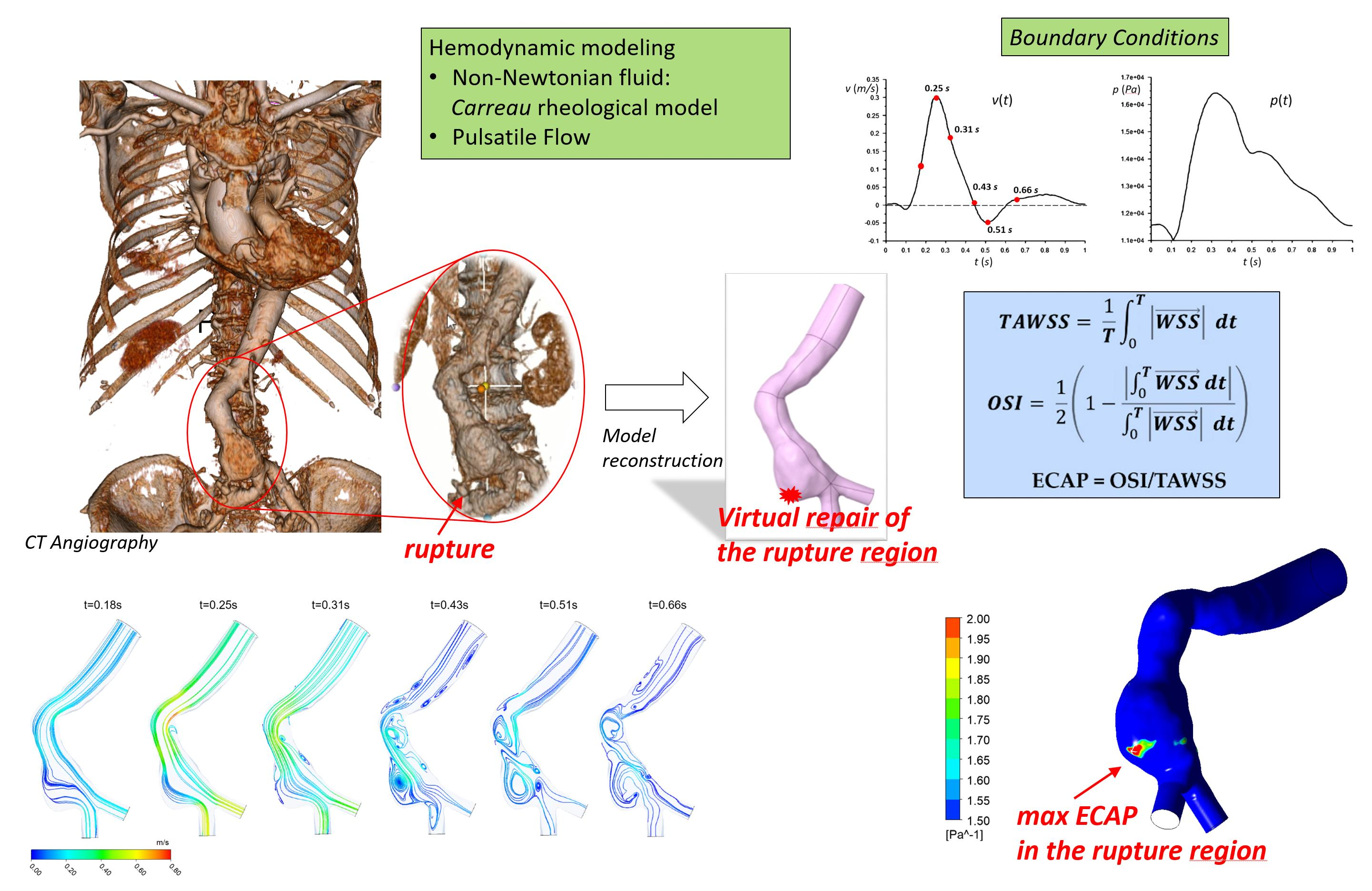
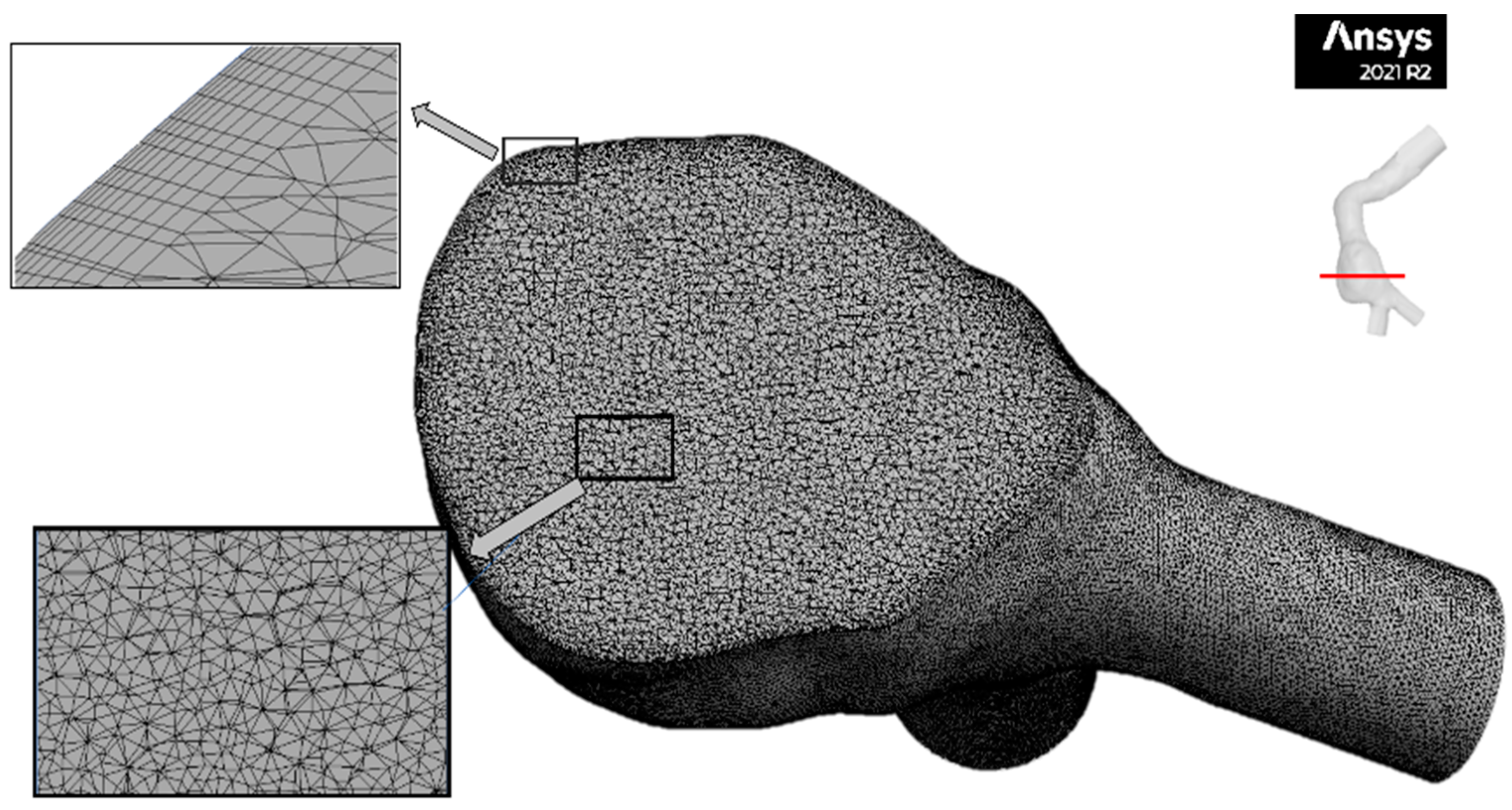
2.1. Pre-Rupture Patient-Specific Model Reconstruction

To simulate the pulsatile blood flow in diseased arteries, accurate reconstruction of the patient-specific model is a fundamental step, as it furnishes the computational domain to be used in the numerical investigation. Incorrect segmentation leads to incorrect hemodynamic analysis which results in wrong conclusions in the assessment of the progression of the disease. The method of reconstruction of the patient-specific geometry from the CT images used in this work is illustrated below.
The AAA model was derived from patient data selected from the clinical case database of the Vascular Surgery Unit, Department of Medicine, Surgery and Neuroscience, University of Siena, Italy. The clinical history was the following. An 81-year-old woman was admitted to the emergency department with abdominal pain. A thoracoabdominal computed tomography angiography was performed, and the exam highlighted the presence of an infrarenal abdominal aortic aneurysm with no radiological signs of rupture or impending rupture. The patient was hospitalized to perform in the following days an endovascular repair of the AAA with the implantation of a bifurcated aortic endograft. [23,24]. In the next hours, the patient started to be hemodynamically unstable with significant hemoglobin loss. In this light, an emergent CT was repeated that revealed a clear rupture of the AAA. The subject gave informed consent to use data for research purposes at the moment of hospital admission. The ethical committee of the hospital was informed of the no-experimental, retrospective analysis of the case, and no objections were raised.
The Angio-CT of the ruptured aneurysm was used for the 3D model reconstruction. As illustrated, the Angio-CT was acquired immediately after the rupture of the aneurysm. Since it is reasonable that the geometry of the aneurysm does not change significantly immediately before and after the rupture, the CT scans of the ruptured aneurysm were considered representative of the conditions immediately preceding the rupture. Based on this assumption, the ITK-SNAP software (v.3.8.0) was used for the segmentation process, in order to reconstruct the pre-rupture geometry, i.e., the geometry that immediately precedes the rupture. Therefore, a first coarse model of the luminal surface of the rupturing patient-specific aneurysm was obtained. The region of rupture, which corresponds to the leakage of blood, was artificially closed and smoothed, by the Meshmixer 3.5 software (http://www.meshmixer.com/ (accessed on 7 October 2021) Autodesk, Inc., San Rafael, CA, USA). In this step of model reconstruction, visceral arteries and minor arteries that branch off the aorta were occluded to simplify the model, and the blood flow was confined into the aorta.
A further pre-processing phase of the aneurysm model reconstruction was made using the open-source VMTK software (Vascular Modeling Tool Kit, version 1.4.0) in order to obtain the final geometry of the pre-rupture aneurysm. In this step, a global smooth of the luminal surface was made, and cylindrical flow extensions were added at the inlet and outlets of the patient-specific model. The insertion of the artificial extensions reduces boundary effects on numerical results and allows the flow to become fully developed before affecting the aneurysmal dilatation [25,26].
The final refined model, in STL format, reflects all the patient-specific morphological features of the examined abdominal aneurysm and allows analyzing the effects of hemodynamics on its rupture. Once the preliminary process on medical images was completed, the specific geometry of the aneurysm was imported into SpaceClaim software (ANSYS Inc., 2020 R2), which allowed extracting surfaces from the STL file. The main steps of the aneurysm model reconstructions and the final pre-rupture geometry are shown in Figure 1.

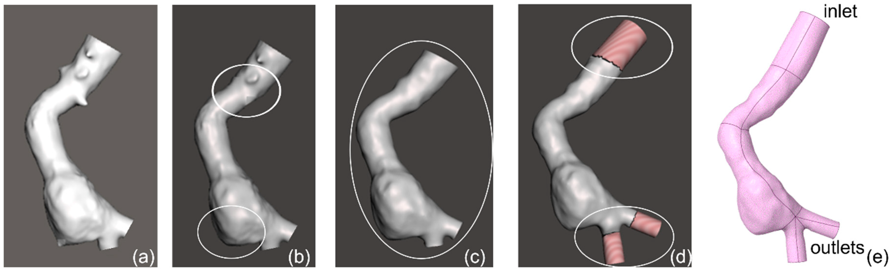
2.2. Governing Equations and Numerical Setup

To achieve reliable results on the influence of hemodynamics on the growth and rupture of abdominal aortic aneurysms, numerical simulations of blood flow in aneurysms must be carried out considering the complexity of the physical problem. In the abdominal artery, the flow is pulsating, the blood is characterized by non-Newtonian rheological behavior, and the patient-specific aneurysmal geometries are extremely complex and must be accurately reconstructed. The above considerations were taken into account in the present computational investigations.
The governing equations of the fluid dynamics problem are the mass and momentum conservation equations, which for incompressible fluid and negligible gravity force are [25]:
· u = 0  
ρ ( u t   +   u u )   =   p + · τ
where u is the velocity vector, p the pressure, and ρ the density of the fluid. The deviatoric stress tensor τ   is a function of the strain rate tensor D , according to the relation τ = 2   μ (   γ ˙ )   D , where μ is the dynamic viscosity of the fluid, γ ˙ is the shear rate, and D = (∇ u +∇ u   T)/2.
The assigned boundary conditions are: u = 0 on the wall of the patient-specific model (no-slip condition), a flat (plug) velocity profile v = v(t) normal to the inlet section, and a time-dependent pressure p = p(t) at the outlet sections (Figure 2).
The system of Equations (1) and (2), with the associate boundary and initial conditions, determines the blood flow. It was numerically solved using the computational fluid dynamics software ANSYS Fluent (v. 2021 R2). A first order implicit method was used for the discretization of the temporal terms, the SIMPLE (Semi-Implicit Method for Pressure Linked Equations) scheme was used for the pressure-velocity coupling, and a second order upwind scheme was selected for the spatial discretization of momentum [19,27,28,29].
Furthermore, the following assumptions were adopted. Blood was modelled as an incompressible fluid, characterized by a non-Newtonian behavior, due to both its composition of suspended cells and the ability of red blood cells to deform and aggregate. The shear-thinning behavior of blood was modelled by the Carreau model. Thus, the following relationship holds for the dynamic viscosity µ:
μ ( γ ˙ ) = μ + ( μ 0 μ ) [ 1 + ( λ γ ˙ ) 2 ] n 1 2  
where μ0 = 0.056 kg/(m·s) is the viscosity at zero shear rate γ ˙ , μ = 0.0035 kg/(m·s) is the viscosity for an infinite shear rate, λ = 3.313 is the relaxation time, and n = 0.3568 is the power-law index [30].
A laminar flow condition was assumed. This assumption is suggested by the low value of the average Reynolds number Re = ρUD/µ, where D is the diameter of the healthy aorta at the inlet of the model (D = 0.024 m), and U is the time averaged velocity (U = 0.09 m/s) assigned at the inlet where a velocity distribution constant along the radial direction was assumed. Assuming the blood density ρ = 1060 kg/m3 and the dynamic viscosity µ = 0.0035 kg/(m·s), the Reynolds number is approximately Re ≈ 680. The maximum Reynolds number, corresponding to the systolic peak velocity, is equal to 2190. This value is less than 2300 which is the threshold for turbulence of Newtonian steady flow in pipes, when Poiseuille’s law holds. In this study, unsteady pulsatile flow conditions of a non-Newtonian fluid are considered. Thus, the laminar flow condition is only a reasonable assumption, frequently used in hemodynamic investigations of the abdominal aortic aneurysm [19,27,31,32].
The unsteady nature of the pulsatile blood flow was modelled by assigning appropriate physiological boundary conditions at the inlet and the outlets of the patient specific model. In particular, a pulsating flow was set at the inlet of the model and a pressure pulse at the iliac outlets. Due to the fact that the patient-specific velocity and pressure waveforms were not available, typical pulses of the abdominal aortic segment, derived from the literature [33], were assigned at the inlet of the model (Figure 2). As shown in Figure 2, peak systolic velocity occurs at t = 0.25 s, and a reverse flow condition is observed at the diastolic minimum instant t = 0.51 s. Other instants were considered for the computational simulations, as they were significant for the evolution of the hemodynamic field. In particular, they refer to the systolic acceleration phase (t = 0.18 s), the deceleration phase (t = 0.31 s and t = 0.43 s), and the diastolic acceleration phase (t = 0.66 s) (Figure 2).
Figure 2. (a) Pulsatile velocity waveform assigned at the inlet of the model, (b) pressure waveform assigned at the outlets of the model. Red points indicate the instants of the cardiac cycle selected for the numerical investigation.
Fluids 07 00269 g002
Furthermore, a no-slip condition was imposed on the walls, and the aneurysm wall was assumed to be rigid, due to the fact that abdominal aortic aneurysms become stiffer with the progression of the disease [5,34]. This last assumption is also supported by degradation of elastin and increase in collagen fibers of the aortic wall that characterize the aneurysm growth [35,36,37].
In this perspective, numerical simulations were performed under pulsatile flow conditions, using the representative vascular geometry obtained from the segmentation process. A computational mesh was generated with the ANSYS meshing software, with a refinement near the wall in order to capture the high velocity gradients in that area (Figure 3).
The number of mesh elements can greatly affect the accuracy of the numerical solutions. Therefore, a mesh sensitivity analysis was performed, with element size ranging from 1.3 mm to 0.42 mm, to ensure the numerical results were not sensitive to the mesh size. In particular, the maximum values of the Time Averaged Wall Shear Stress (TAWSS) evaluated at the third numeric cycle was monitored for the different mesh size. Between the last two values, only 1.5% variation was found (Table 1).
Moreover, for different sizes of the mesh elements, the velocity profiles, plotted in section A-A passing from the healthy aorta to the aneurysm, were compared at the instant of the systolic peak of the pulsatile motion (Figure 4). As the element size decreased, a minor discordance among the velocity profiles was observed. The good correspondence in the velocity distributions for the lower values of the element size, shown in Figure 3, highlighted the independence of the solutions from the number of computational cells and suggested the choice of the element size of the mesh. Therefore, a maximum size of 0.42 mm was selected for the mesh elements, which corresponds to 3,486,569 elements in the mesh. The element size and the number of elements obtained from the sensitivity analysis are similar to what others have reported for similar cases [31,38,39,40].
The time step used for numerical integration was equal to 0.005 s, and 200 time steps were necessary to represent cardiac cycle, which was equal to 1 s. A time-step independence was assumed at the selected time step, in line with similar studies in the literature [32,41,42]
A maximum value of 200 iterations were performed for each time step. The threshold value for residual error convergence of velocity components and continuity was set as 10−5. The numerical investigations were carried out for three cycles in order to minimize the influence of initialization effects, but only the third cycle was analyzed.

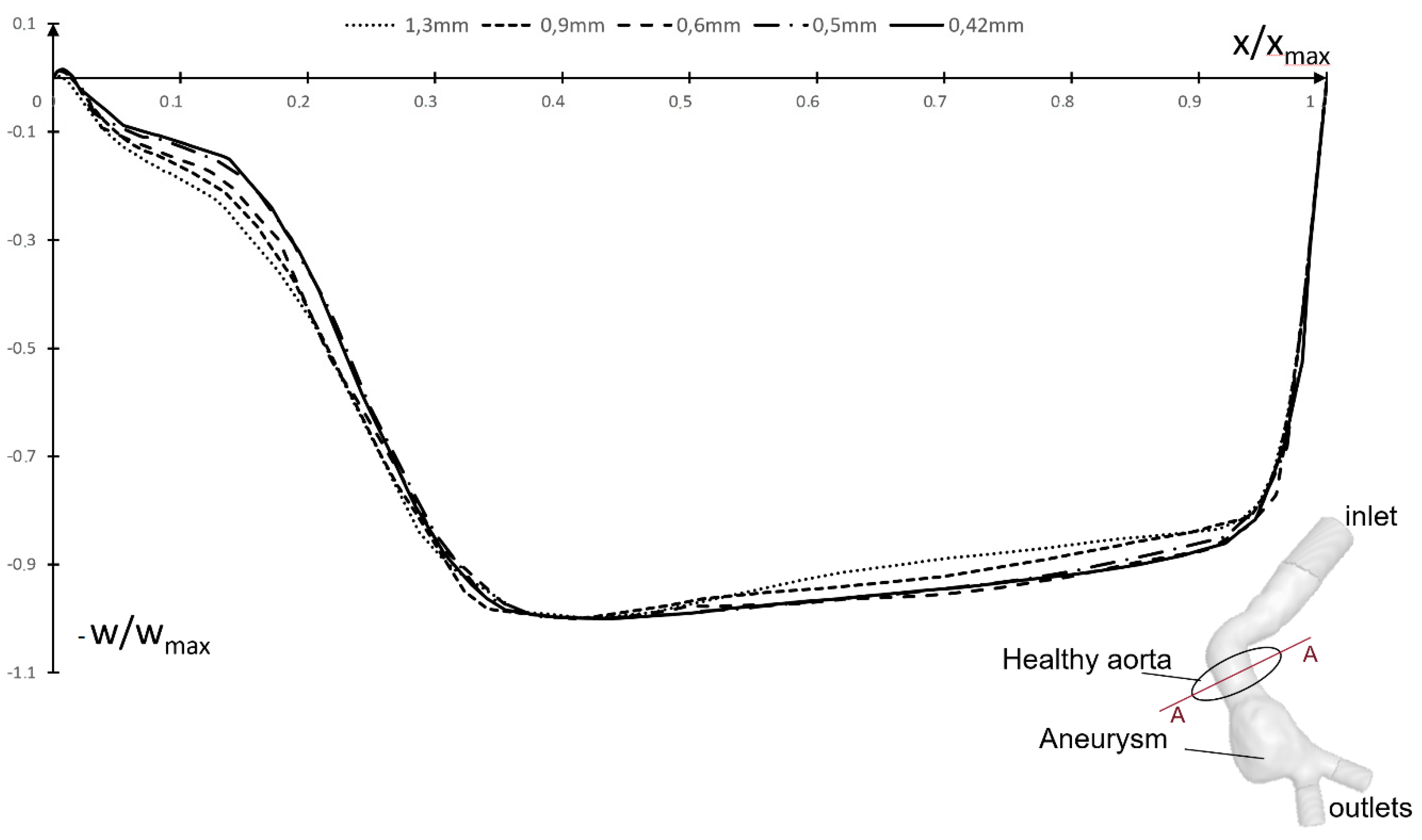
2.3. Hemodynamic Parameters

To furnish useful information on the hemodynamic field in the pre-rupture model of the patient-specific aneurysm, 2D and 3D streamline evolutions as well as the instantaneous WSS contours were analyzed at the selected significant instants of the cardiac cycle shown in Figure 2. Moreover, the hemodynamic indicators TAWSS, OSI and ECAP were calculated. These parameters are able to characterize significantly the unsteady nature of the flow in the diseased artery and to identify areas of potential rupture. In particular, the time averaged wall shear stress TAWSS furnishes the average over the cardiac cycle of the magnitude of WSS vector:
TAWSS = 1 T 0 T | W S S |   d t
where T is the period of the cardiac cycle, and W S S indicates the instantaneous WSS vector.
The oscillatory shear index OSI takes into account changes in the direction of the WSS vector with respect to the dominant direction of the flow during the cardiac cycle [15]:
OSI = 1 2 ( 1 | 0 T W S S   d t | 0 T | W S S |   d t )
Values of OSI range from 0 to 0.5, where 0 indicates unidirectional shear stress. High OSI value has been recognized as inducing an inflammatory response of the artery wall, while unidirectional shear stress is related to a healthy condition [20]. Moreover, a positive correlation between OSI and ILT growth was found [43].
The endothelial cell activation potential ECAP relates TAWSS and OSI through ratio of the two indices and characterizes the degree of ‘thrombogenic susceptibility’ of the vessel wall [38]:
ECAP = OSI/TAWSS
This index is generally used to locate areas of the arterial wall that are exposed to both high OSI and low TAWSS at the same time. High ECAP values correspond to large OSI and small TAWSS, that is, conditions of endothelial susceptibility [38].

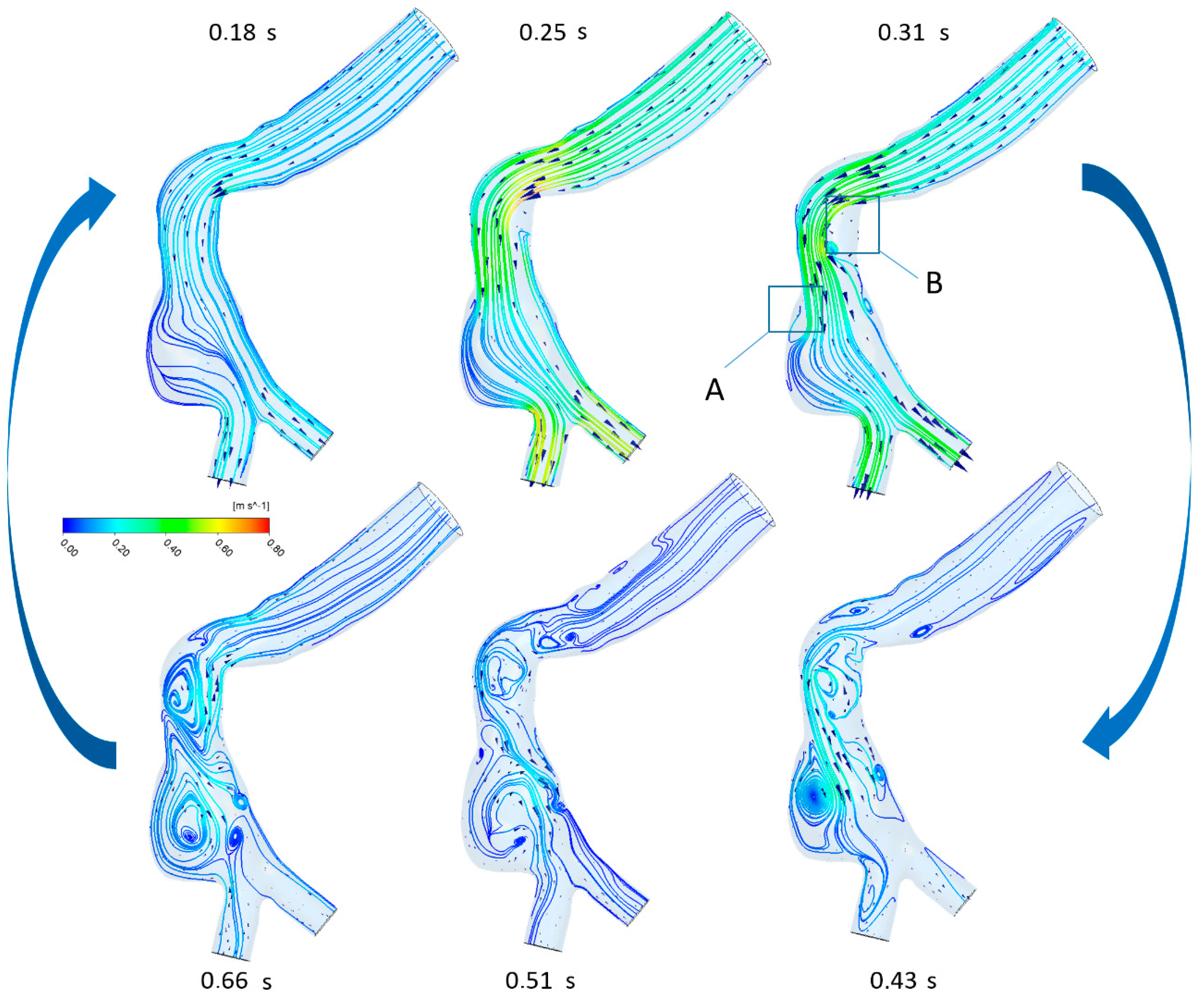
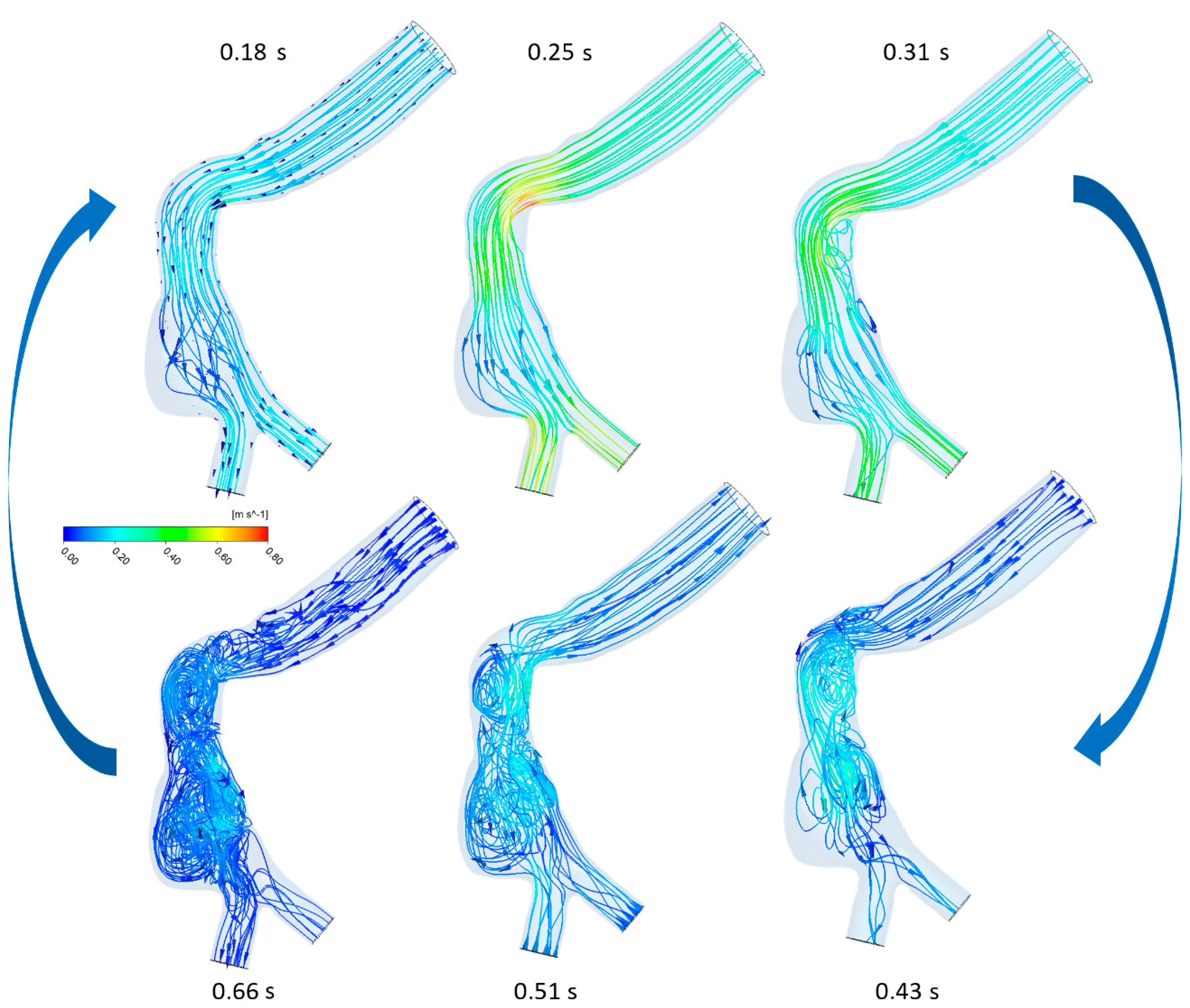
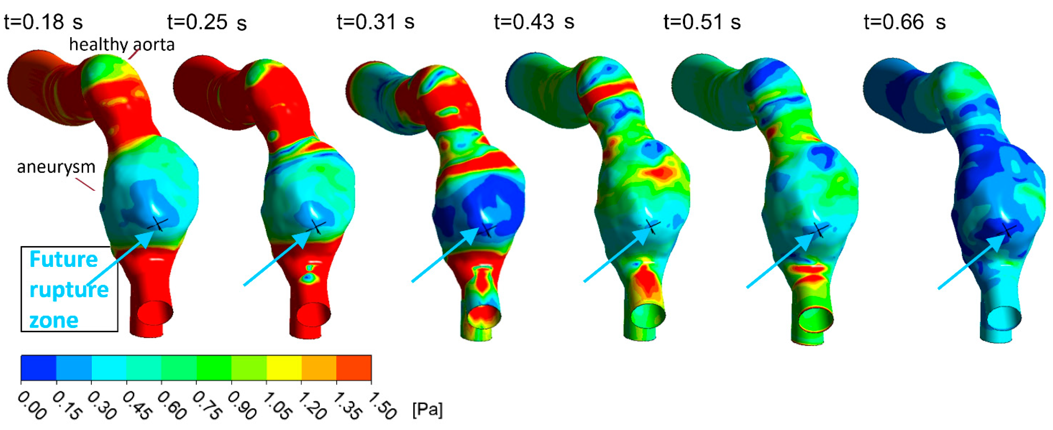
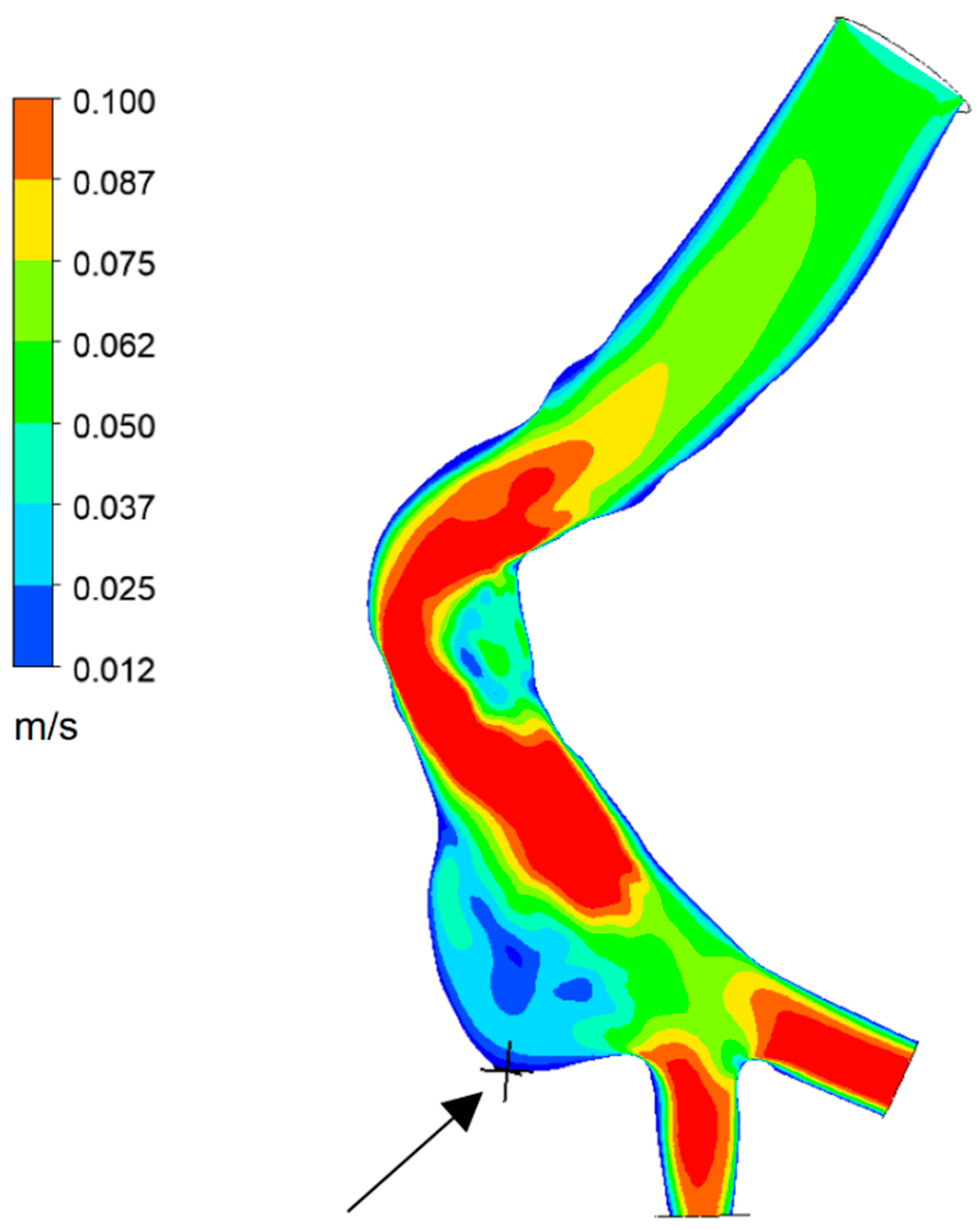
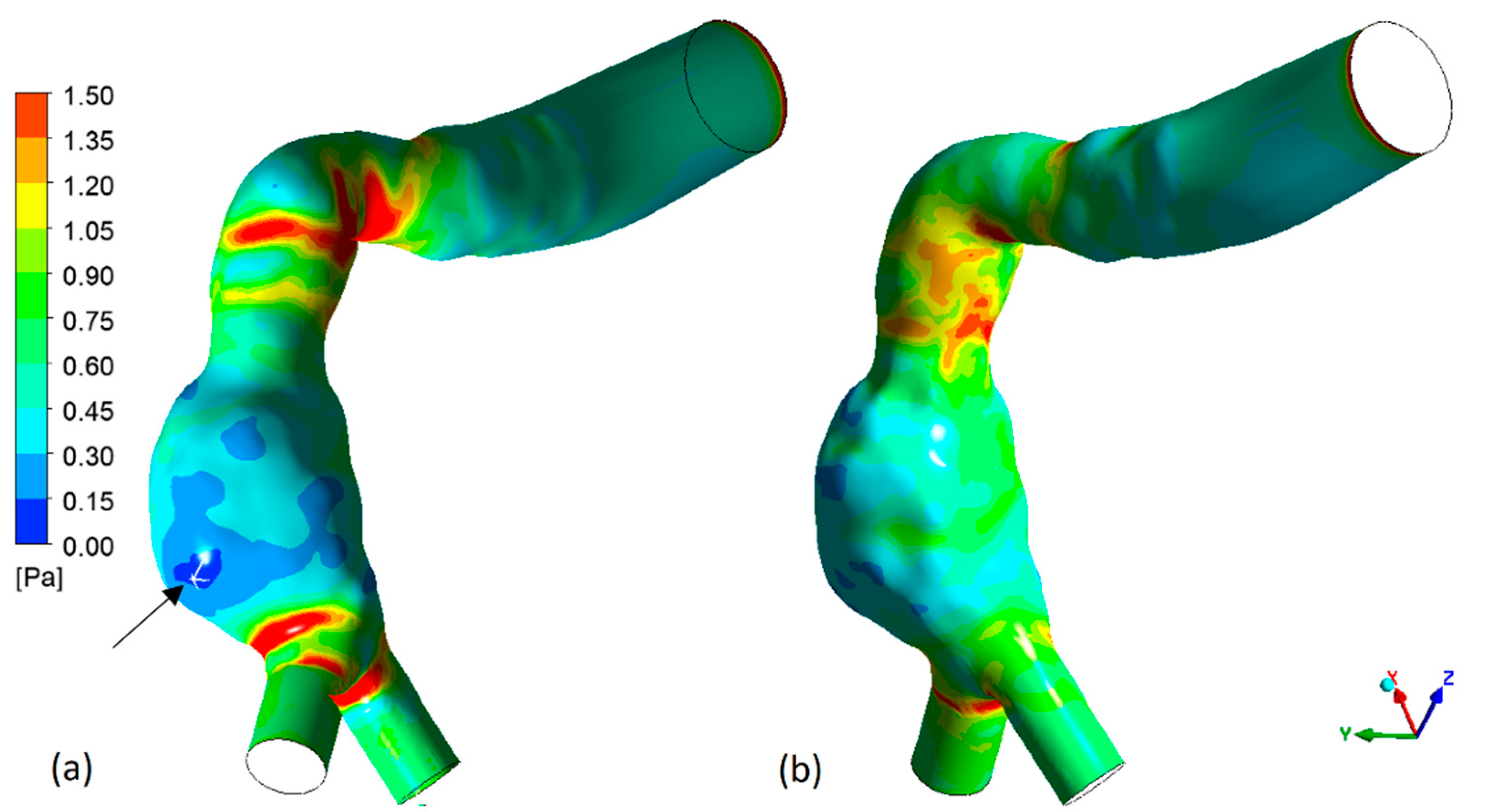
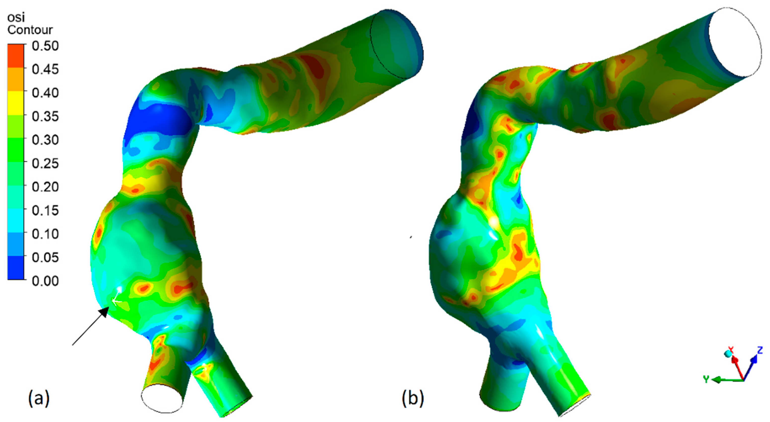
3. Results and Conclusions

Non-Newtonian pulsatile blood flow in the rupturing patient-specific aneurysm was numerically investigated to evaluate the effect of hemodynamics on the evolution of the disease. Due to the fact that the rupture zone of the aneurysm was artificially repaired, fundamental information was known about the incipient rupture in the analyzed geometry and the location of the rupture zone. Consequently, the link between the flow patterns and the rupture of the aneurysm could be investigated to establish the role of hemodynamic parameters in predicting the rupture of the abdominal aortic aneurysm.
The results of the numerical simulations are shown below. In particular, the temporal evolution of 2D and 3D streamlines in the pre-rupture model of the aneurysm was analyzed to understand how flow patterns and recirculation regions develop in time (Figure 5 and Figure 6). The 2D and 3D streamlines were examined in the same representative phases of the cardiac cycle (Figure 2a). The 2D streamlines refer to a longitudinal section of the aneurysm, which was chosen to capture the maximum area of the dilatation in the direction of the mean flow and to highlight the blood flow around the rupture zone.
The geometry of the considered aneurysm was characterized by high surface complexity and tortuosity, which significantly affected the blood motion. At the selected instants of the cardiac cycle, different flow patterns were observed. In the first instants of the phase of systolic acceleration, the residual vortices emerging from the previous cycle were quickly suppressed by the accelerating flow and were not found in the aneurysm, even if a helical flow persists (Figure 5 and Figure 6, t = 0.18 s).
As the systolic peak was reached, the flow velocity increased significantly, highlighting the maximum values (Figure 5 and Figure 6, t = 0.25 s). Despite this temporal acceleration, the enlargement of the vessel leads to a consistent spatial deceleration in the bulge with respect to the flow condition in the healthy aorta region. The consequent increase in pressure determines the separation of the flow within the dilatation already at the first instants of the deceleration phase (Figure 5 and Figure 6, t = 0.31 s). This is highlighted by the small recirculation area originating in the region of the most significant widening of the aneurysm, marked with A in Figure 5 (t = 0,31 s). At the same time, a consistent vortical flow originated in the healthy aorta upstream of the aneurysm, due to the detachment of the fluid in correspondence with the pronounced angle of the vessel (region B in Figure 5, t = 0,31 s).
In the following phase of the cardiac cycle, the inlet velocity reaches zero values, and the vortices gradually reduce their velocities but widen, affecting the entire bulge of the aneurysm and a large region of the upstream non-dilated aorta (Figure 5 and Figure 6, t = 0.43 s). The vanishing of the inlet velocity at this instant contributes to the onset of a strongly disturbed blood flow in the vessel, with a large number of new vortices in the healthy aorta slowly recirculating.
In the successive diastolic phase, a retrograde flow interacts with the preexisting vortices, determining the weakening of the larger recirculation regions and the disappearance of the smaller vortices close to the wall (Figure 5 and Figure 6, t = 0.51 s and t = 0.66 s). In the later phases of the cardiac cycle, the vortices decrease in number and gradually disappear when a subsequent cycle starts.
Figure 5. 2D streamlines on the longitudinal cross-section of the patient-specific model of the rupturing aneurysm at the selected instants of the cardiac cycle. In the figure, the recirculation areas in the aneurysm and the healthy aorta are indicated respectively with the letters A and B.
Fluids 07 00269 g005
Figure 6. 3D streamlines at the selected instants of the cardiac cycle.
Fluids 07 00269 g006
The spatial distributions of WSS were analyzed during the cardiac cycle, since low and oscillating WSS characterizing the pulsatile motion seems to be associated with possible rupture of the aneurysm [27,29,44]. The 3D streamlines’ evolution during the cardiac cycle is simulated in Video S1.
The understanding of the flow evolution during the cardiac cycle is significant, because recirculating blood associated with low TAWSS have been considered as responsible for the deterioration of the arterial wall [16,17,18,19]. In particular, the dynamics of the recirculation regions give rise to non-physiological WSS that in turn appears to be negatively correlated with ILT accumulation [19,43] and disruption of artery wall integrity [45]. Moreover, regions characterized by low WSS and high OSI are susceptible to thrombus deposition and consequently to a higher risk of rupture [40]. Lastly, low and oscillating WSS characterizing the pulsatile motion was associated with possible rupture of the aneurysm [27,29,44,46].
Taking into account the above consideration, the instantaneous WSS distributions at the selected instants of the cardiac cycle, TAWSS, OSI and ECAP distributions, were determined in the present study.
Figure 7 shows the instantaneous WSS contours obtained from the computational simulations for the image-based reconstructed model of the pre-rupture aneurysm at the selected instants of the cardiac cycle.
The temporal and spatial distribution of WSS inside the rupturing abdominal aortic aneurysm was due to its specific geometry, which caused flow separation and the consequent emergence of recirculation regions. As highlighted in Figure 7, an altered WSS was found in the aneurysm concerning the physiological values that characterize the non-diseased artery. During the entire cycle, lower WSS compared with the values in the healthy aorta were found on the aneurysmal wall, in agreement with literature results [44,46,47]. Relatively high values characterized the proximal and distal regions of the aneurysm. High WSS were also found in the iliac arteries, due to their tortuosity and the narrowing of the vessels, but these areas are not of interest in this study.
It is interesting to note that, at the instant of systolic peak (t = 0.25 s) the healthy arterial wall was associated with an extremely high WSS that decayed in the subsequent instants. Furthermore, at any instant of the cardiac cycle, there were always minimum relative values around the area of the incipient rupture (Figure 5). During the systolic deceleration phase (t = 0.31s), the WSS values in the bulge significantly decreased around the future rupture region but assumed high values in the region of high curvature at the inlet of the dilatation.
At the diastolic minimum, i.e., t = 0.51 s, the retrograde flow, although associated with low velocities, interacted with the pre-existing vortical flow, determining local small increases in WSS. Finally, at the diastolic acceleration phase, t = 0.66s, the WSS values decrease drastically in the bulge.
To describe in more detail the interaction between pulsating blood flow and possible rupture of the aneurysm, the spatial distribution of fundamental hemodynamic quantities, averaged over the entire cardiac cycle, was analyzed, i.e., distribution of time-averaged velocity, TAWSS, OSI and ECAP.
Figure 8 illustrates time-averaged velocity contours on the longitudinal cross-section of the patient-specific model of the rupturing aneurysm. Figure 9, Figure 10 and Figure 11 show the TAWSS, OSI and ECAP on the luminal surfaces for the patient-specific aneurysm examined in the pre-rupture condition.
The results of the numerical simulations indicated regions of slow recirculation flows and low values of Time Averaged Wall Shear Stress (TAWSS) in the region of rupture (Figure 6 and Figure 7). Unlike literature results, high Oscillatory Shear Index (OSI) was not clearly found in this region, and further regions of high OSI values were detected that were not linked to the ruptured zone (Figure 8).
Nevertheless, just in the region where the rupture will occur, the maximum value of the Endothelial Cell Activation Potential index (ECAP) was found (Figure 9), and, unlike what happens when analyzing TAWSS and OSI contour maps, no uncertainty arises regarding further possible areas of rupture of the aneurysm. This index is therefore extremely significant for assessing the vulnerability of the aortic wall and locating the critical rupture region.
In the present study, the wall of the aneurysm was assumed rigid, as widely accepted in the literature [32,39,46,47,48]. The hypothesis is due to the increase in wall stiffness of the abdominal aortic aneurysm AAAs with the progression of the disease [5,34]. In support of this, degradation of elastin and increase in collagen fibers of the wall have been found in the development of the aortic aneurysm [35,36,37]. On the other hand, fluid–structure interaction models, which take into account the elasticity of the wall, require patient-specific parameters, e.g., artery wall stiffness or thrombus properties, difficult to evaluate. However, in future research, it might be of interest to consider the elasticity of blood vessels in the analysis of the earlier stages of the disease.
Another limitation in this study is the assumption of non-patient-specific velocity and pressure pulses. As the patient-specific data were not available, only typical pulses of the abdominal aortic segment were used to model blood flow. In this regard, although more accurate results could be achieved with patient-specific boundary conditions, some limitations however could occur, related to the spatial resolution of the current imaging techniques, such as 4D MRI. Moreover, it does not provide information on the pressure field [49].
Despite the above limitations, this study highlights the importance of hemodynamics in assessing the vulnerability of the aortic wall. Moreover, it furnishes a contribution to identifying significant parameters for the prediction of the risk of aneurysm rupture as an alternative to the criterion of maximum diameter, supporting the clinical management of AAA disease.

Supplementary Materials

The following supporting information can be downloaded at: https://www.mdpi.com/article/10.3390/fluids7080269/s1, Video S1: 3D streamlines’ evolution during the cardiac cycle.

Author Contributions

Conceptualization, M.A.B. and M.C.C.; methodology, M.A.B. and M.C.C.; software, M.A.B., M.C.C. and R.M.; validation, M.A.B. and M.C.C.; formal analysis, M.A.B. and R.M.; investigation, M.C.C.; resources, G.d.D. and E.P.; writing—original draft preparation, M.A.B. and M.C.C.; writing—review and editing, M.A.B., M.C.C., R.M., E.P. and G.d.D.; supervision, M.A.B. and G.d.D.; project administration, M.A.B.; funding acquisition G.d.D. All authors have read and agreed to the published version of the manuscript.

Funding

This research received no external funding.

Institutional Review Board Statement

Not applicable.

Informed Consent Statement

Informed consent was obtained from all subjects involved in the study.

Data Availability Statement

Not applicable.

Conflicts of Interest

The authors declare no conflict of interest.

References

  1. Solomon, C.G.; Kent, K.C. Abdominal aortic aneurysms. New Engl. J. Med. 2014, 371, 2101–2108. [Google Scholar] [CrossRef]
  2. Gopalakrishnan, S.S.; Pier, B.; Biesheuvel, A. Dynamics of pulsatile flow through model abdominal aortic aneurysms. J. Fluid Mech. 2014, 758, 150–179. [Google Scholar] [CrossRef] [Green Version]
  3. Chaikof, E.L.; Dalman, R.L.; Eskandari, M.K.; Jackson, B.M.; Lee, W.A.; Mansour, M.A.; Mastracci, T.M.; Mell, M.; Murad, M.H.; Nguyen, L.L.; et al. The Society for Vascular Surgery practice guidelines on the care of patients with an abdominal aortic aneurysm. J. Vasc. Surg. 2018, 67, 2–77. [Google Scholar] [CrossRef] [PubMed] [Green Version]
  4. Wanhainen, A.; Verzini, F.; Van Herzeele, I.; Allaire, E.; Bown, M.; Cohnert, T.; Dick, F.; van Herwaarden, J.; Karkos, C.; Koelemay, M.; et al. Editor’s Choice—European Society for Vascular Surgery (ESVS) 2019 Clinical Practice Guidelines on the Management of Abdominal Aorto-iliac Artery Aneurysms. Eur. J. Vasc. Endovasc. Surg. 2019, 57, 8–93. [Google Scholar] [CrossRef] [PubMed] [Green Version]
  5. Vorp, D.A. Biomechanics of abdominal aortic aneurysm. J. Biomech. 2007, 40, 1887–1902. [Google Scholar] [CrossRef] [Green Version]
  6. Huang, Y.; Teng, Z.Z.; Elkhawad, M.; Tarkin, J.M.; Joshi, N.; Boyle, J.R.; Buscombe, J.R.; Fryer, T.D.; Zhang, Y.; Park, A.Y.; et al. High structural stress and presence of intraluminal thrombus predict abdominal aortic aneurysm 18F-FDG uptak. Circ. Cardiovasc. Imaging 2016, 9, 004656. [Google Scholar] [CrossRef] [Green Version]
  7. Haller, S.J.; Crawford, J.D.; Courchaine, K.M.; Bohannan, C.J.; Landry, G.J.; Moneta, G.L.; Azarbal, A.F.; Rugonyi, S. Intraluminal thrombus is associated with early rupture of abdominal aortic aneurysm. J. Vasc. Surg. 2018, 67, 1051–1058. [Google Scholar] [CrossRef] [Green Version]
  8. Laine, M.T.; Vänttinen, T.; Kantonen, I.; Halmesmäki, K.; Weselius, E.; Laukontaus, S.; Salenius, J.; Aho, P.; Venermo, M. Rupture of Abdominal Aortic Aneurysms in Patients Under Screening Age and Elective Repair Threshold. Eur. J. Vasc. Endovasc. Surg. 2016, 51, 511–516. [Google Scholar] [CrossRef] [Green Version]
  9. Nicholls, S.C.; Gardner, J.B.; Meissner, M.H.; Johansen, K.H. Rupture in small abdominal aortic aneurysms. J. Vasc. Surg. 1998, 28, 884–888. [Google Scholar] [CrossRef] [Green Version]
  10. Darling, R.C.; Messina, C.R.; Brewster, D.C.; Ottinger, L.W. Autopsy study of unoperated abdominal aortic aneurysms. The case for early resection. Circulation 1977, 56 (Suppl. S3), II161-4. [Google Scholar]
  11. Vande Geest, J.P.; Di Martino, E.S.; Bohra, A.; Makaroun, M.S.; Vorp, D.A. A biomechanics-based rupture potential index for abdominal aortic aneurysm risk assessment: Demonstrative application. Ann. N. Y. Acad. Sci. 2006, 1085, 11–21. [Google Scholar] [CrossRef] [PubMed]
  12. Maier, A.; Gee, M.W.; Reeps, C.; Pongratz, J.; Eckstein, H.-H.; Wall, W.A. A Comparison of Diameter, Wall Stress, and Rupture Potential Index for Abdominal Aortic Aneurysm Rupture Risk Prediction. Ann. Biomed. Eng. 2010, 38, 3124–3134. [Google Scholar] [CrossRef] [PubMed]
  13. Gijsen, F.; Katagiri, Y.; Barlis, P.; Bourantas, C.; Collet, C.; Coskun, U.; Daemen, J.; Dijkstra, J.; Edelman, E.; Evans, P.; et al. Expert recommendations on the assessment of wall shear stress in human coronary arteries: Existing methodologies, technical considerations, and clinical applications. Eur. Heart J. 2019, 40, 3421–3433. [Google Scholar] [CrossRef] [PubMed] [Green Version]
  14. Chiu, J.J.; Chien, S. Effects of Disturbed Flow on Vascular Endothelium: Pathophysiological Basis and Clinical Perspectives. Physiol. Rev. 2011, 91, 327–387. [Google Scholar] [CrossRef] [PubMed] [Green Version]
  15. Ku, D.N.; Giddens, D.P.; Zarins, C.K.; Glagov, S. Pulsatile flow and atherosclerosis in the human carotid bifurcation. Positive correlation between plaque location and low oscillating shear stress. Arteriosclerosis 1985, 5, 293–302. [Google Scholar] [CrossRef] [Green Version]
  16. Cecchi, E.; Giglioli, C.; Valente, S.; Lazzeri, C.; Gensini, G.F.; Abbate, R.; Mannini, L. Role of hemodynamic shear stress in cardiovascular disease. Atherosclerosis 2011, 214, 249–256. [Google Scholar] [CrossRef]
  17. Tarbell, J.M.; Shi, Z.D.; Dunn, J.; Jo, H. Fluid mechanics, arterial disease, and gene expression. Annu. Rev. Fluid Mech. 2014, 46, 591–614. [Google Scholar] [CrossRef] [Green Version]
  18. Takehara, Y.; Isoda, H.; Takahashi, M.; Unno, N.; Shiiya, N.; Ushio, T.; Goshima, S.; Naganawa, S.; Alley, M.; Wakayama, T.; et al. Abnormal flow dynamics result in low wall shear stress and high oscillatory shear index in abdominal aortic dilatation: Initial in vivo assessment with 4D-flow MRI. Magn. Reson. Med. Sci. 2020, 19, 235–246. [Google Scholar] [CrossRef]
  19. Kelsey, L.J.; Powell, J.T.; Norman, P.E.; Miller, K.; Doyle, B.J. A comparison of hemodynamic metrics and intraluminal thrombus burden in a common iliac artery aneurysm. Int. J. Numer. Methods Biomed. Eng. 2017, 33, e2821. [Google Scholar] [CrossRef] [Green Version]
  20. Sorescu, G.P.; Song, H.N.; Tressel, S.L.; Hwang, J.; Dikalov, S.; Smith, D.A.; Boyd, N.L.; Platt, M.O.; Lassègue, B.; Griendling, K.; et al. Bone morphogenic protein 4 produced in endothelial cells by oscillatory shear stress induces monocyte adhesion by stimulating reactive oxygen species production from a nox1-based NADPH oxidase. Circ. Res. 2004, 95, 773–779. [Google Scholar] [CrossRef] [Green Version]
  21. Arzani, A.; Suh, G.-Y.; Dalman, R.L.; Shadden, S.C. A longitudinal comparison of hemodynamics and intraluminal thrombus deposition in abdominal aortic aneurysms. Am. J. Physiol. Heart Circ. Physiol. 2014, 307, H1786–H1795. [Google Scholar] [CrossRef] [PubMed]
  22. O'Rourke, M.J.; McCullough, J.P.; Kelly, S. An investigation of the relationship between hemodynamics and thrombus deposition within patient-specific models of abdominal aortic aneurysm. Proc. Inst. Mech. Eng. Part H J. Eng. Med. 2012, 226, 548–564. [Google Scholar] [CrossRef] [PubMed]
  23. Pasqui, E.; de Donato, G.; Giannace, G.; Panzano, C.; Setacci, C.; Palasciano, G. Management of abdominal aortic aneurysm in nonagenarians: A single-centre experience. Vascular 2021, 29, 27–34. [Google Scholar] [CrossRef] [PubMed]
  24. de Donato, G.; Pasqui, E.; Nano, G.; Lenti, M.; Mangialardi, N.; Speziale, F.; Ferrari, M.; Michelagnoli, S.; Tozzi, M.; Palasciano, G.; et al. Long-term results of treatment of infrarenal aortic aneurysms with low-profile stent grafts in a multicenter registry. J. Vasc Surg. 2022, 75, 1242–1252.e2. [Google Scholar] [CrossRef] [PubMed]
  25. Schlichting, H. Boundary Layer Theory, 7th ed.; McGraw-Hill: New York, NY, USA, 1979. [Google Scholar]
  26. Wood, N.B. Aspects of fluid dynamics applied to the larger arteries. J. Biol. 1999, 199, 137–161. [Google Scholar] [CrossRef] [PubMed]
  27. Boyd, A.J.; Kuhn, D.C.S.; Lozowy, R.J.; Kulbisky, G.P. Low wall shear stress predominates at sites of abdominal aortic aneurysm 460 rupture. J. Vasc. Surg. 2016, 63, 1613–1619. [Google Scholar] [CrossRef] [Green Version]
  28. Ferziger, J.H.; Peric, M. Computational Methods for Fluid Dynamics; Springer: Berlin/Heidelberg, Germany, 2001; ISBN 978-3-540-42074-3. [Google Scholar]
  29. Forneris, A.; Marotti, F.B.; Satriano, A.; Moore, R.D.; Di Martino, E.S. A novel combined fluid dynamic and strain analysis approach identified abdominal aortic aneurysm rupture. J. Vasc. Surg. Cases Innov. Tech. 2020, 6, 172–176. [Google Scholar] [CrossRef]
  30. Shibeshi, S.S.; Collins, W.E. The rheology of blood flow in a branched arterial system. Appl. Rheol. 2005, 15, 398–405. [Google Scholar] [CrossRef]
  31. Zambrano, B.; Gharahi, H.; Lim, C.; Jaberi, F.; Choi, J.; Lee, W.; Baek, S. Association of intraluminal thrombus, hemodynamic forces, and abdominal aortic aneurysm expansion using longitudinal CT images. Ann. Biomed. Eng. 2016, 44, 1502–1514. [Google Scholar] [CrossRef]
  32. Qiu, Y.; Wang, Y.; Fan, Y.B.; Peng, L.; Liu, R.; Zhao, J.; Yuan, D.; Zheng, T. Role of intraluminal thrombus in abdominal aortic aneurysm ruptures: A hemodynamic point of view. Med. Phys. 2019, 46, 4263–4275. [Google Scholar] [CrossRef]
  33. Xenos, M.; Rambhia, S.H.; Alemu, Y.; Einav, S.; Labropoulos, N.; Tassiopoulos, A.; Ricotta, J.J.; Bluestein, D. Patient-based abdominal aortic aneurysm rupture risk prediction with fluid structure interaction modeling. Ann. Biomed. Eng. 2010, 38, 3323–3337. [Google Scholar] [CrossRef]
  34. Vande Geest, J.P.; Sacks, M.S.; Vorp, D.A. The effects of aneurysm on the biaxial mechanical behavior of human abdominal aorta. J. Biomech. 2006, 39, 1324–1334. [Google Scholar] [CrossRef] [PubMed]
  35. Thubrikar, M.J.; Labrosse, M.; Robicsek, F.; Al-Soudi, J.; Fowler, B. Mechanical properties of abdominal aortic aneurysm wall. J. Med. Eng. Technol. 2001, 25, 133–142. [Google Scholar] [CrossRef] [PubMed]
  36. Tong, J.; Cohnert, T.; Holzapfel, G.A. Diameter-related variations of geometrical, mechanical, and mass fraction data in the anterior portion of abdominal aortic aneurysms. Eur. J. Vasc. Endovasc. Surg. 2015, 49, 262–270. [Google Scholar] [CrossRef] [PubMed] [Green Version]
  37. Kolipaka, A.; Illapani, V.S.P.; Kenyhercz, W.; Dowell, J.D.; Go, M.R.; Starr, J.E.; Vaccaro, P.S.; White, R.D. Quantification of abdominal aortic aneurysm stiffness using magnetic resonance elastography and its comparison to aneurysm diameter. J. Vasc. Surg. 2016, 64, 966–974. [Google Scholar] [CrossRef] [PubMed] [Green Version]
  38. Di Achille, P.; Tellides, G.; Figueroa, C.A.; Humphrey, J.D. A haemodynamic predictor of intraluminal thrombus formation in abdominal aortic aneurysms. Proc. R. Soc. Lond Math. Phys. Eng. Sci. 2014, 470, 20140163. [Google Scholar] [CrossRef] [Green Version]
  39. Lozowy, R.J.; Kuhn, D.C.S.; Ducas, A.A.; Boyd, A. The relationship between pulsatile flow impingement and intraluminal thrombus deposition in abdominal aortic aneurysms. Cardiovasc. Eng. Technol. 2017, 8, 57–69. [Google Scholar] [CrossRef]
  40. Les, A.S.; Shadden, S.C.; Figueroa, C.A.; Park, J.M.; Tedesco, M.M.; Herfkens, R.J.; Dalman, R.L.; Taylor, C.A. Quantification of hemodynamics in abdominal aortic aneurysms during rest and exercise using magnetic resonance imaging and computational fluid dynamics. Ann. Biomed. Eng. 2010, 38, 1288–1313. [Google Scholar] [CrossRef]
  41. Poelma, C.; Watton, P.N.; Ventikos, Y. Transitional flow in aneurysms and the computation of haemodynamic parameters. J. R. Soc. Interface 2015, 12, 20141394. [Google Scholar] [CrossRef]
  42. Tan, F.P.P.; Borghi, A.; Mohiaddin, R.H.; Wood, N.B.; Thom, S.; Xu, X.Y. Analysis of flow patterns in a patient-specific thoracic aneurysm model. Comput. Struct. 2009, 87, 680–690. [Google Scholar] [CrossRef]
  43. Tzirakis, K.; Kamarianakis, Y.; Metaxa, E.; Kontopodis, N.; Ioannou, C.V.; Papaharilaou, Y. A robust approach for exploring hemodynamics and thrombus growth associations in abdominal aortic aneurysms. Med. Biol. Eng. Comput. 2017, 55, 1493–1506. [Google Scholar] [CrossRef]
  44. Doyle, B.J.; McGloughlin, T.M.; Kavanagh, E.G.; Hoskins, P.R. From detection to rupture: A serial computational fluid dynamics case study of a rapidly expanding, patient-specific, ruptured abdominal aortic aneurysm. In Computational Biomechanics for Medicine: Fundamental Science and Patient-Specific Applications; Doyle, B., Miller, K., Wittek, A., Eds.; Springer: Berlin/Heidelberg, Germany, 2014; pp. 53–68. [Google Scholar] [CrossRef]
  45. Koole, D.; Zandvoort, H.J.A.; Schoneveld, A.; Vink, A.; Vos, J.A.; Hoogen, L.L.V.D.; de Vries, J.-P.P.; Pasterkamp, G.; Moll, F.L.; van Herwaarden, J.A. Intraluminal abdominal aortic aneurysm thrombus is associated with disruption of wall integrity. J. Vasc. Surg. 2013, 57, 77–83. [Google Scholar] [CrossRef] [Green Version]
  46. Boniforti, M.A.; Di Bella, L.; Magini, R. On the role of hemodynamics in predicting rupture of the abdominal aortic aneurysm. J. Zhejiang Univ. Sci. A 2021, 22, 957–978. [Google Scholar] [CrossRef]
  47. Soudah, E.; Ng, E.Y.K.; Loong, T.H.; Bordone, M.; Pua, U.; Narayanan, S. CFD modelling of abdominal aortic aneurysm on hemodynamic loads using a realistic geometry with CT. Comput. Math. Methods Med. 2013, 2013, 472564. [Google Scholar] [CrossRef]
  48. Patel, S.; Usmani, A.Y.; Muralidhar, K. Effect of aorto-iliac bifurcation and iliac stenosis on flow dynamics in an abdominal aortic aneurysm. Fluid Dyn. Res. 2017, 49, 035513. [Google Scholar] [CrossRef]
  49. Canchi, T.; Kumar, S.D.; Ng, E.Y.K.; Narayanan, S. A review of computational methods to predict the risk of rupture of abdominal aortic aneurysms. BioMed Res. Int. 2015, 2015, 861627. [Google Scholar] [CrossRef] [Green Version]
Figure 1. Main steps of the patient-specific aneurysm reconstruction from the Angio-CT medical images of a ruptured aneurysm: (a) rough segmentation (ITK_SNAP), (b) virtual repair and cut of minor arteries (Meshmixer), (c) global smooth (VMTK) (d) insertion of extensions (VMTK), (e) surface extraction (SpaceClaim).
Fluids 07 00269 g001
Figure 3. Mesh cross section through the aneurysm in the central region and enlarged view near the wall highlighting the local refinement.
Fluids 07 00269 g003
Figure 4. Dimensionless w-velocity at systolic peak instant (t = 0.25 s), plotted in section A-A passing from the healthy aorta to the aneurysm, for different sizes of the mesh element: 1.3 mm, 0.9 mm, 0.6 mm, 0.5 mm, and 0.42 mm.
Fluids 07 00269 g004
Figure 7. WSS contours distribution in the rupturing aneurysm at the selected instants of the cardiac cycle (t = 0.18 s, t = 0.25 s, t = 0.31 s, t = 0.43 s, t = 0.51 s, and t = 0.66 s). The arrow and the black cross indicate the future rupture point.
Fluids 07 00269 g007
Figure 8. Time-averaged velocity contours on the longitudinal cross-section of the rupturing aneurysm. The arrow and the black cross indicate the region where rupture really occurred (future rupture region).
Fluids 07 00269 g008
Figure 9. TAWSS contours distribution on the luminal surfaces of the rupturing aneurysm: (a) front view, (b) back view. The arrow and the white cross indicate the region where rupture really occurred (future rupture region).
Fluids 07 00269 g009
Figure 10. OSI contours distribution on the luminal surfaces of the rupturing aneurysm: (a) front view, (b) back view. The arrow and the white cross indicate the region where rupture really occurred (future rupture region).
Fluids 07 00269 g010
Figure 11. ECAP contours distribution on the luminal surfaces of the rupturing aneurysm: (a) front view, (b) back view. The arrow and the white cross indicate the region where rupture really occurred (future rupture region).
Fluids 07 00269 g011
Table 1. Maximum TAWSS values at the third numeric cycle for different mesh size.
Mesh Element Size (mm)TAWSS (Pa)
1.32.78073
0.92.91181
0.62.98067
0.53.10283
0.423.05512
Publisher’s Note: MDPI stays neutral with regard to jurisdictional claims in published maps and institutional affiliations.

