1. Introduction
Sediment transport commonly occurs in unlined water conveyance systems such as rivers, streams, canals, and drainage channels. There are three sediment transport modes: wash load, bedload, and suspended load. In wash load, particles do not exist on the bed, therefore, the characterization and prediction of wash load composition is highly difficult. The bedload transfer is almost always in contact with the bed. Bedload transport takes place if critical friction velocity (
) is less than the friction velocity (
). The suspended load, which is part of the total load, moves without continuously being in contact with the bed. Turbulence is the main flow property that keeps the sediment in suspension [
1,
2,
3]. The turbulence is characterized by the magnitude of root mean square velocity (
). For significant suspension to occur
near the bed must exceed the sediment fall velocity (
). Sediment particle concentration distribution along the depth is very important for predicting the sediment transport rate that is taking place in the river. However, the problem with suspended load transport is that it is not fully understood, because of limitations in modelling techniques such as diffusion theory [
4]. Rouse [
5] developed a suspended sediment concentration profile based on diffusion theory for steady uniform flows by using the eddy viscosity model to relate Reynolds stress and log-law for the velocity profile. Despite the drawbacks of diffusion theory, the Rouse model has become a standard for calculating suspended sediment concentration profiles and a basis for many models developed later.
Two-phase flows have complex interactions between the phases. Modelling fluid–particle interactions and particle–particle attractions is difficult therefore they are excluded. Huang et al. [
6], Hsu et al. [
7] and Rouse [
5] resolved this issue based on the differential continuity equation of suspended sediment diffusion in the 2D steady turbulent flow. They considered that the sediment diffusion coefficient is related to both the mixing length and the turbulence intensity. These models could not account for turbulence or forces operating on the sediment particle surfaces, such as collisions between particles, and as a result, their accuracy was limited. To overcome this, several studies have addressed sediment distributions in stationary and uniform two-dimensional (2D) open channel flows by solving the momentum equation for sediment particles [
4,
8,
9]. Most notably, the diffusion coefficient of sediment particles generated from the momentum conservation equation provides significantly more accurate, perhaps allowing for a better understanding of sediment particle dispersion. Generally, the sediment concentration profile attains the maximum at some distance above the bed surface, decreases with farther moving away from the bed, and finally attains the minimum at the free surface. To model suspended-sediment distribution along with the depth, parameters such as particle fall velocity, particle diameter, turbulence intensity, shear velocity, Rouse number and mean concentration are required [
10,
11]. Kundu and Ghosal [
4] and Pu and Lim [
12] found that two-dimensional incompressible flow modelling over a sediment bed with a uniform slope predicts reasonably accurate suspended sediment transport since full three-dimensional modelling involves a lot more complexity. In addition, the diffusion theory with appropriate modifications such as a two-layer theoretical model based on diffusion theory or the fractional advection-diffusion equation can predict suspended sediment concentration profiles with reasonable accuracy. Goree et al. [
13] used equations of motion and considered drift flux, which is a fluid that consists of multiple phases or volume fractions. The mixture flow consists of different volume fractions and each volume fraction has a different transport velocity. This velocity depends on the particle size and the total volumetric concentration of solids. Goree et al. [
13] used LES for turbulence modelling however the computed results were not accurate at the wall. Another type of modelling concept is kinetic theory. Models established based on kinetic theory for granular flows and two-fluid models i.e., the probability density function (PDF) approach, in which both fluid and solid phases are considered as continuum media, allow classic continuum mechanics to be naturally employed to formulate the two-phase flows with fundamental conservation laws [
4]. Therefore, the observable macro mechanical states of flows and sediment transport are completely determined by conservation equations of solid and liquid systems. In addition, other theories, such as a numerical investigation based on the kinetic theory of granular flows, in combination with a RANS (Reynolds-Averaged Navier–Stokes) turbulence model were investigated by Ekambara et al. [
14] for a pipe flow using Ansys CFX which gave very good results. Ni et al. [
10] developed a combined model of both kinetic theory and diffusion theory, which has given reasonable results.
The limitations of existing models to simulate suspended sediment transport can be efficiently overcome with data-driven models such as machine learning. Barati et al. [
15] estimated the drag coefficient of a smooth sphere using multi-gene genetic programming. Alizadeh et al. [
16] used ANN and Bayesian network models to predict pollutant transport in natural rivers. Sadeghifar and Barati [
17] used soft-computing techniques with very good accuracy to predict sediment transport in the southern shorelines of the Caspian Sea. Cao et al. [
18] developed a nonparametric machine-learning (ML) model to predict the settling velocity of noncohesive sediment which demonstrated the capability of the ML model for accuracy and consistency. Rushd et al. [
19] used AI-based machine learning algorithms to develop a generalized model for computing the settling velocity of spheres in both Newtonian and non-Newtonian fluids. The above-mentioned studies demonstrate that data-driven models (AI and ML) and soft-computing techniques are powerful tools for predicting complicated processes such as sediment transport.
A central perspective advocated in this paper is that by exploiting foundational knowledge of suspended sediment profiles and physical constraints, data-driven approaches can be used to yield useful predictive results. In this paper, current models are analysed and the crucial flow parameters are estimated by using machine learning algorithms.
2. Model Review
The diffusion theory was utilised by van Rijn [
20], Wang and Ni [
21], McLean [
22], and Zhong et al. [
23] to define the transport of suspended material in numerical modelling. According to diffusion theory, sediment transport takes place from higher concentration areas to lower concentration areas [
24]. Rouse [
5] derived suspended sediment concentration in a steady uniform current. As per Rouse [
5], the sediment is kept in suspension mainly by turbulence [
7]. Rouse [
5] used Prandtl’s mixing length theory to estimate the vertical profile of suspended sediment. Rouse’s [
5] methodology is given as follows.
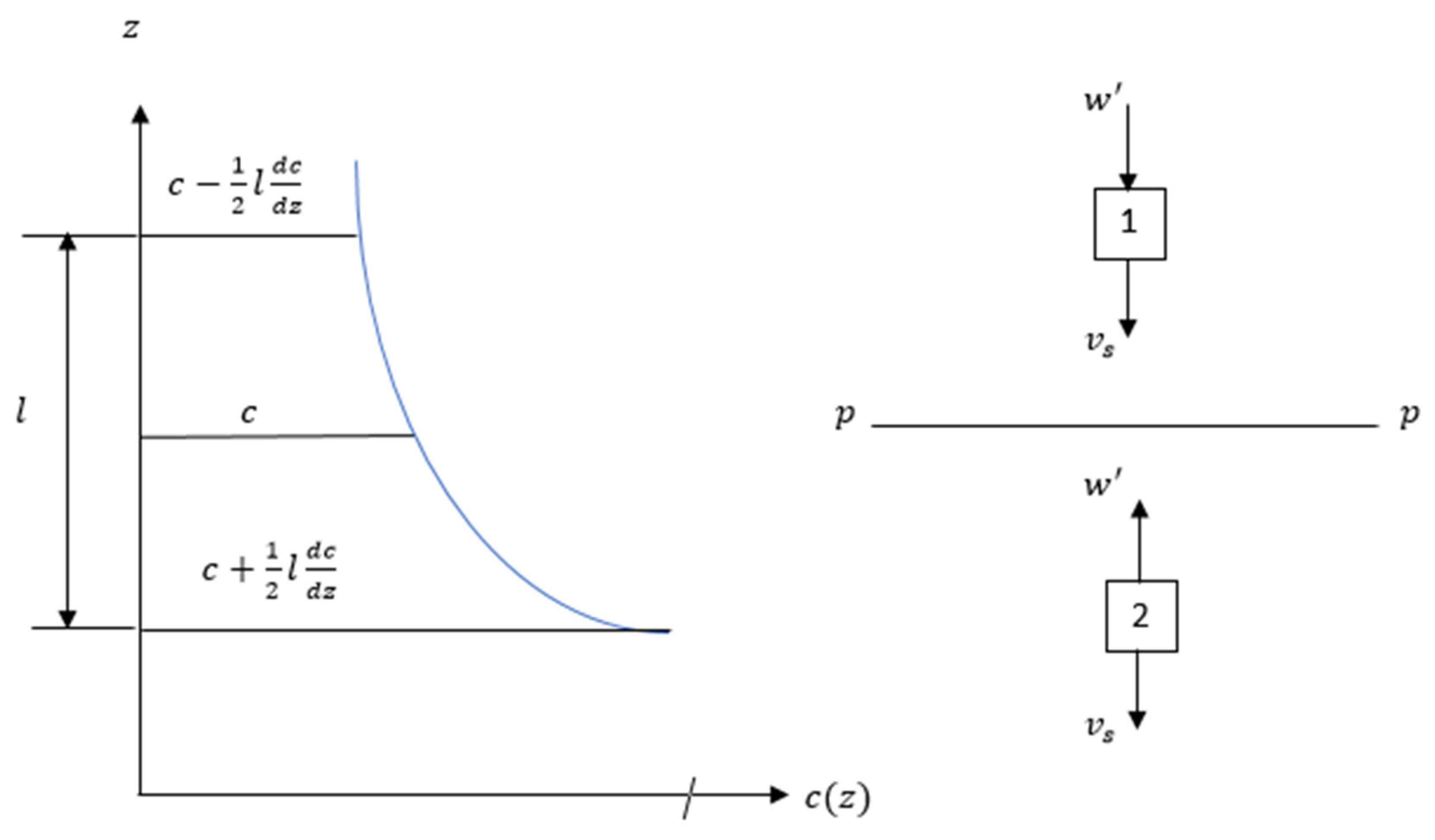
As shown in
Figure 1, consider two sand particles 1 and 2 with a settling velocity
. In a unit time through a unit area on horizontal plan p-p, the sediment volumes going up (
) and down (
) are:
In an equilibrium state,
and
must be equal to each other, substracting Equation (2) from Equation (1) gives
By assuming that
where mixing length
,
0.4 and
= friction velocity,
= flow depth.
Substituting Equation (3) into Equation (4) yields
By integrating Equation (5), one obtains
where
is the integration constant (
) and
Rouse number (
). It is assumed that bedload transport takes place in the bedload layer from
0 to
. In the bedload layer, sediment concentration is given by
. Hsu et al. [
7] suggested
is approximately 0.005. The concentration distribution profile is thought to grow more uniform, according to Rouse [
5]. Small settling velocity and minimal shear velocity can result in low Rouse numbers.
Log-law can be written as
The flux per river cross-section per square meter can be written from Equations (7) and (8) as
For steady, uniform open channel flow, the sediment concentration varies with the distance from the wall. The depth can be nondimensionalized as where its range is .
In addition, Kundu and Ghosal [
11] recognized that sediment concentration profiles occur in three (type I, type II, and type III) types as shown in
Figure 2. For the low-flow condition, the sediment carrying capacity is weak, therefore the maximum concentration occurs at the bed and decreases exponentially to the minimum concentration at the free surface. This type of profile is called type I. In medium-flow conditions, the sediment concentration is lower near the bed because of the gravity effect, sediment concentration attains a maximum concentration a little distance away from the bed and is the lowest near the free surface, and is classified as type II. The type III profile is attained during high-flow conditions subjected to hyper concentration. In the type III profile, sediment concentration is low near the bed as well as near the free surface, whereas the maximum concentration occurs in the middle region. According to Kundu and Ghoshal [
11], the entire flow depth can be divided into two regions: the inner suspension region, where sediment concentration increases with a characteristic height from the sediment bed (
). Here
corresponds to
and
corresponds to the nondimensional height at which the suspended sediment starts. The outer suspension region above the inner suspension region, where sediment concentration decreases with an increase in the characteristic height and
. For each region, sediment concentration which is a function of characteristic height can be written as
where
are experimental coefficients that can be found by the least squares method by analysing observed data.
In the asymptotic matching method (refer
Figure 3), the final model of suspended sediment concentration for the entire flow region is given as follows [
25].
The aforementioned equation has also been used by Bouvard and Petkovic [
26], Wang and Ni [
21], and Einstein and Chein [
27] to demonstrate that the sediment profile for a diluted flow should follow a power law (Equations (10) and (11)). In Equations (10) and (11),
= 0 produce a simplified form of power law as given below.
Equation (13) is similar to Rouse Equation (Equation (7)). For type III, the sediment transport equation in power-law format is not suitable. Pu et al. [
1] stated that the linear-type profile fits well. Therefore, the equation for the suspended sediment profile for type III is given as follows
This is similar to Equations (7) and (8) but
value is taken as unity. Rouse formulation has drawbacks at the riverbed and the free surface as shown by the experimental studies of Kironoto and Yulistiyanto [
28], Goeree et al. [
13], Greiimann and Holly [
8], Jha and Bombardelli [
9], and Sumer et al. [
29]. Since the Rouse formula is derived from the diffusion theory, it is valid only for a single phase i.e., sediment phase. Therefore, the Rouse formula is applicable only for the type I profile with zero concentration at the free surface and infinite concentration at the bed [
30]. According to Huang et al. [
6], the Rouse formula produces an inaccurate estimation of sediment concentration near the bed for highly rough conditions. Kumbhakar et al., [
30] showed that the Rouse formula can be improved by incorporating an additional factor to dampen the diffusion coefficient. Sumer et al. [
29] tried to improve the reference height representation to better estimate suspended sediment modelling. Greiimann and Holly [
8] stated that the Rouse formula excluded the particle–particle attractions in addition to the assumption in estimating diffusion coefficient resulting Rouse formula valid only for
. Rouse formula gives a good understanding as long as sediment particles have small inertia. Wang and Ni [
21], Ni et al. [
10], and Zhong et al. [
23] models showed significant differences in the shape of the vertical profile. The concentration calculated by the Wang model changes slowly under 0.05 h but the Rouse model changes dramatically. The Zhong model, the power-law model, the Rouse model, and the two-phase flow model provide similar results near the water’s surface.
The proposed study will look into the relationships between different flows and sediment factors to better describe them in Equations (10)–(12). This will result in a parameterized expression of the final characteristic model for suspended particles and enable accurate profile prediction. Rouse number , size parameter , and mean concentration are the flow parameters that will be examined.
3. Proposed Model
Numerous studies have examined the factors that should be taken into account when determining a concentration profile, such as Rouse number, particle size, mean concentration, and flow depth [
5,
29,
31,
32]. By using a modified Equation (12), the variables that are thought to be connected to the power-linear law coefficients are as follows:
where
is the diameter of the sediment particle,
is the mean concentration,
is the Rouse number,
is the flow depth, and
is the size parameter (
). In order to examine the distribution of each power-linear law coefficient toward the physical parameters of Rouse number, particle size, and mean concentration and to derive a modified Rouse model for validation tests, we collected the data from numerous reported experimental studies (as detailed in
Table 1).
Table 1 further shows that the data sources employed to cover a broad range of tested parameters. Particularly, the range of
in the referenced literature is from 0.00013 to 0.147, which provides an accurate picture of flow conditions from diluted to hyper-concentrated.
3.1. Machine-Learning Algorithms
In trying to investigate the relationship between power-linear law coefficients of the Kundu and Ghoshal model and sediment parameters such as the Rouse number, particle size, mean concentration, and flow depth, various machine-learning models have been used as follows:
3.1.1. XGboost Classifier
XGBoost is a decision-tree-based ensemble machine-learning technique that uses gradient boosting. It may be used to solve a variety of regression and classification predictive modelling challenges. It is a fast implementation of the stochastic gradient boosting algorithm with several hyperparameters that allows the fine tuning of the model’s training process.
3.1.2. Linear Regressor (Ridge)
Linear regression uses a best-fit straight line to establish a link between a dependent variable () and one or more independent variables () (also known as a regression line). Ridge regression is a multicollinear data analysis technique (independent variables are highly correlated).
3.1.3. Linear Regressor (Bayesian)
While Ridge regression utilises L2 norm regularisation, Bayesian regression is a probabilistic linear regression model with explicit priors on the parameters. Priors can have a regularising impact, for example, the application of Laplace priors for coefficients is comparable to L1 regularisation.
3.1.4. K Nearest Neighbours
The supervised machine learning algorithm K-nearest neighbours (kNN) can be used to address both classification and regression problems. Because it delivers highly precise predictions, this algorithm can compete with the most accurate models. As a result, the kNN algorithm can be utilised in applications where great accuracy is required but a human-readable model is not required. The accuracy of the predictions is influenced by the distance measured.
3.1.5. Decision Tree Regressor
In the corporate world, the Decision Tree algorithm has become one of the most widely utilised machine learning algorithms. Both classification and regression issues can benefit from the use of the Decision Tree. In the shape of a tree structure, the Decision Tree constructs regression or classification models. It incrementally cuts down a dataset into smaller and smaller sections while also developing an associated decision tree. A tree with decision nodes and leaf nodes is the result.
3.1.6. Support Vector Machines (Regressor)
SVM stands for Support Vector Machine and is a supervised machine learning method capable of classification, regression, and even outlier detection. SVM classifiers have a high level of accuracy and can anticipate events quickly. They also utilise less memory in the decision phase because they only use a subset of training points. With a clear separation margin and a large dimensional space, SVM performs well.
The complete flow chart describing the workflow of using machine-learning algorithms for estimating coefficients for linear and power laws is shown in
Figure 4.
3.2. Theoretical Description of Proposed Models
The three broad categories of machine-learning approaches are supervised, unsupervised, and semi-supervised learning. Classified data is needed in supervised learning systems so that the algorithm may be trained. In contrast, the unsupervised learning approach discovers features in the data sets without requiring training data to be classified beforehand. These methods have been practised and are well established. While supervised and unsupervised learning techniques are combined in semi-supervised learning systems. The theoretical foundation of the suggested ML models is provided in the paragraph below in this subsection.
Adaptive Boosting (AdaBoost), a very popular boosting technique, focuses on combining several weak classifiers into a single strong classifier. It is the first binary classification boosting ensemble model. It applies to problems involving classification and regression. It can handle both textual and numerical data and is versatile. It is more susceptible to data noise and outliers than XGBoost is. It is more adaptable since it can be used to improve the weak classifiers’ accuracy. In contrast to XGBoost, it minimises exponential loss function rather than differentiable loss function.
CatBoost, an ML algorithm is based on gradient-boosted decision trees. During the model’s training, a collection of decision trees are built one after another. Compared to the prior trees, the loss decreases with each additional tree. The gradient boosting method is the foundation for the CatBoost Regressor implementation, which uses a decision tree as the primary predictor. Because there is not a sparse dataframe, the data, which contains many categorical features, is processed much more quickly than it would be if another technique, such XGBoost or Random Forest was being used. In CatBoost, parameters self-tune to save time modifying. With CatBoost, we can work more effectively with ML engineers and software engineers because we can essentially maintain the feature or column in its original state.
The K nearest neighbours (KNN), is a straightforward machine learning algorithm that examines all of the inputs and predicts the target based on features that are similar to them. As a nonparametric model, it has been used in statistical estimation and pattern recognition for more than 50 years. According to this method, the analyst must specify the neighbourhoods’ size. To set the size that lowers the MSE to a minimal amount, cross-validation may also be used. Utilizing an inverse distance weighted average of the KNN is a straightforward use of KNN regression. It makes use of the same KNN classification distance functions. Equations (16)–(18) are used to represent the distance functions.
These three distance functions are applicable only for continuous variables while in the case of discrete or categorical data, the Hamming distance function is used. The Hamming distance function is given below by Equation (19) as:
The Hamming distance function is zero if , otherwise if (), it is equal to unity.
LightGBM, a decision-tree-based gradient boosting framework helps GPU learning while also maximising model efficiency by growing trees vertically (leaf-wise split), as opposed to other boosting approaches that grow trees horizontally, which increases accuracy (level-wise split). Since it transforms continuous values into discrete bins, the primary benefit of the LightGBM regressor is that it lowers memory usage without sacrificing forecasting speed or prediction accuracy.
3.3. Rouse Number Modelling
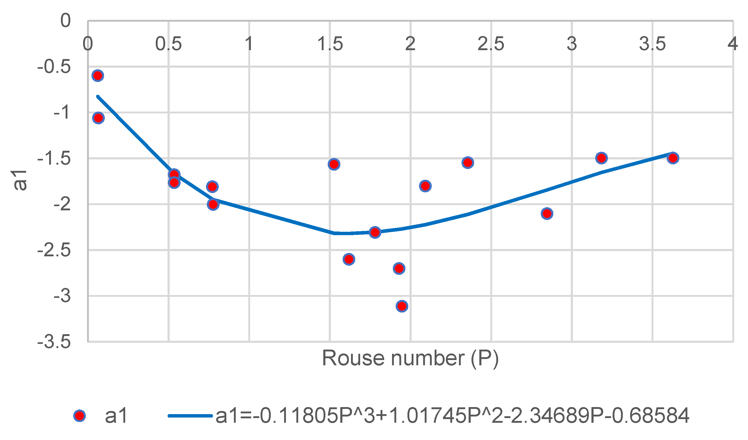
Shear velocity and settling velocity are the two key variables that influence drag on a sediment particle. The Rouse number as stated in Equation (6) is a dimensionless form of these parameters along with the von Karman constant. We may create the figures shown in
Figure 5,
Figure 6,
Figure 7 and
Figure 8 below by testing each value in Equation (12) against
.
Figure 5,
Figure 6,
Figure 7 and
Figure 8 show the relationship between
,
,
and
against
. This result demonstrates that for a wide range of measured data,
offers a reasonable match which is represented by the power law and its coefficients.
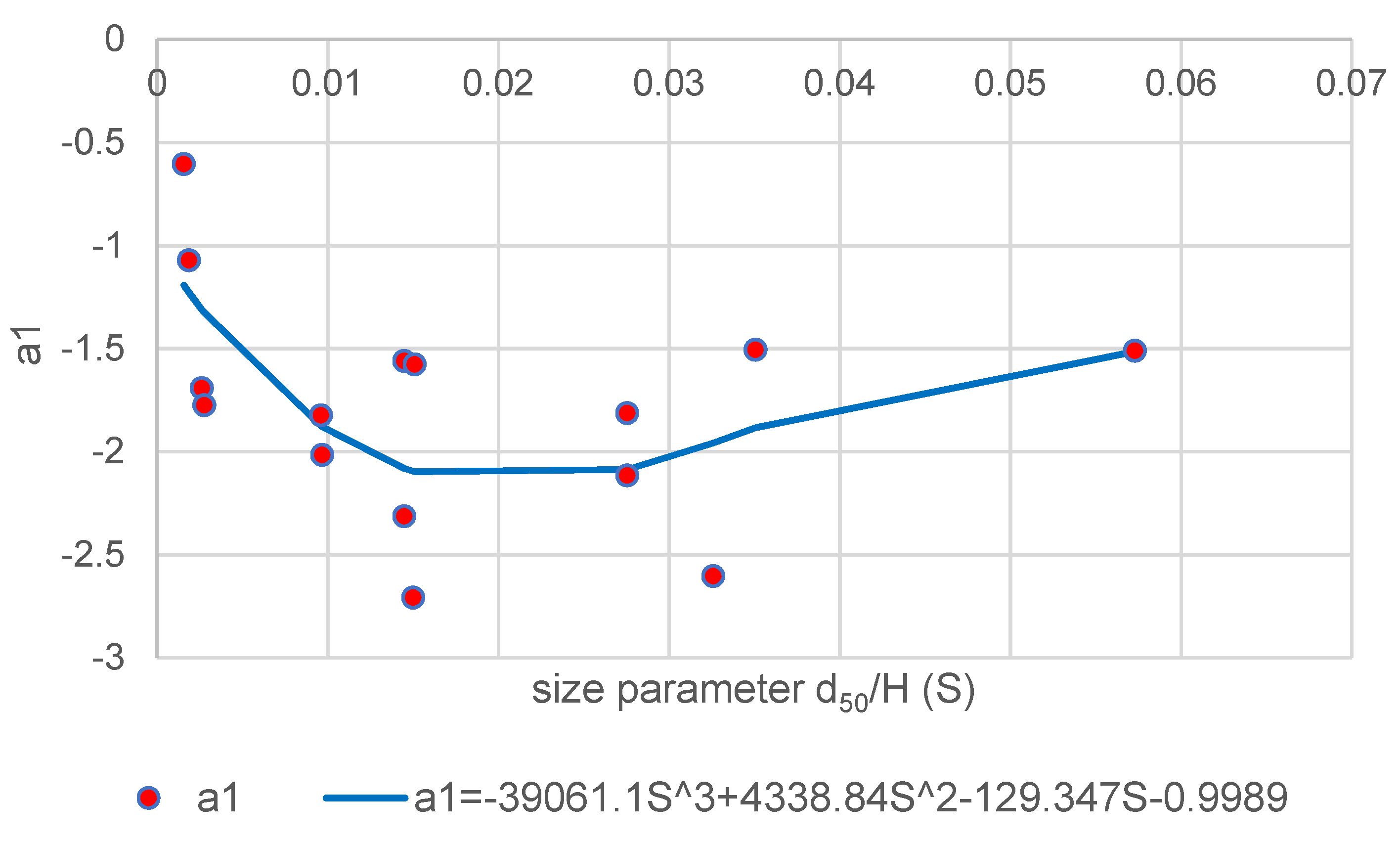
3.3.1. Size Parameter Modelling
Another element that may impact sediment drag and lift is particle size. The effectiveness of interactive interactions acting on the particle can be influenced by the surface area of the particle, which is dictated by the diameter. The settling velocity of a particle is also influenced by its diameter [
35]. The dimensionless
is utilised to model against the power-law coefficients in
Figure 9,
Figure 10,
Figure 11 and
Figure 12 in this study. The effect of particle size has not been taken into account in the modified Rouse model [
11] or the original Rouse technique [
5] despite the fact that it is an important aspect that affects the behaviour of suspended sediment.
The relationship between
,
,
and
against
is depicted in
Figure 9,
Figure 10,
Figure 11 and
Figure 12. Numerous analytical modelling studies, such as Wang and Ni [
21] and Ni et al. [
10], used a coefficient from the concentration equation that was deduced from the collected data to fit the particle diameter. Their experiments demonstrated that when different sediment diameters are investigated, it is challenging to capture the character of the concentration profile. This serves as more evidence of how challenging it is to identify a representative function of the particle size parameter studied here.
3.3.2. Mean Concentration Modelling
For hyper-concentrated flows, the recorded sediment concentration profiles were examined by Cellino and Graf [
33], and Michalik [
36]. Their findings demonstrated that, in contrast to the general power-law shown in earlier studies of diluted flows, the sediment profile for such flows follows a much more uniform and linear distribution. This study will develop the analytical approach by mean concentration to use in linear-law modelling in response to another empirical finding by Michalik [
36] that the mean concentration has a key dominant impact changing the character of concentration distribution when compared to Rouse number and particle size. The fitting between the linear law coefficients and mean concentration was determined using the procedure below, with the findings displayed in
Figure 13,
Figure 14,
Figure 15 and
Figure 16.
The above
Figure 13,
Figure 14,
Figure 15 and
Figure 16 show the relationship between
,
,
, and
. Here, the association between
and the hyper-concentrated profile is evident.
3.3.3. Modified Rouse Approach
Each coefficient is defined in the aforementioned sections before being adapted into Equation (12) to create a parameterized expression for the distribution of silt concentration over the flow depth. A linked approach controls the suggested model for sediment concentration prediction. When
, a power law describes the concentration of diluted silt, whereas a linear law describes the concentration of dense hyper-concentration. This hyper-to-dilute boundary was established by comparing it to the research on diluted flow definition by Greiimann and Holly [
8] and the Rouse model limit. The suggested strategy can be written as in Equation (20).
where
, and
and when
, and
4. Model Validations
The link between parameters of the power-linear coupled model and sediment flow characteristics were discovered using a variety of machine-learning approaches. The distribution of suspended sediment over the characteristic height inside the flow was inclusively estimated from diluted to hyper-concentrated. The model can precisely calculate the suspended sediment profile for a range of flow conditions, and sediment sizes, including a range of Rouse numbers. The models show good accuracy for testing at low and extremely high concentrations for type I to III profiles. The best result-giving model’s RMSE, MAE, and MSE values are displayed in
Table 2.
Initially, the necessary python libraries were imported into the Google Colab environment for modelling. The dataset was then imported using the wget function. The dataset was preprocessed in a suitable format for modelling by separating the X (input feature) and Y (output feature). Using the train-test-split, the dataset was split into train and test sets. Cumulatively we obtained the X_train, Y_train, X_test and Y_test for training and validating the dataset. The models including XGBoost Classifier, Linear Regressor (Ridge), Linear Regressor (BayesianRidge), K-Nearest Neighbours, Decision Tree Regressor and Support Vector Machines (Regressor) were used.
The experimental data from Wang and Qian [
37], Wang and Ni [
31], and Michalik [
36] were used to validate the model proposed in this study (Equation (20)). It was also contrasted with the models that Wang and Ni [
31], Ni et al. [
10], Zhong et al. [
23], and Pu et al. [
1] had previously presented. A theoretical distribution model derived from kinetic theory was presented by Wang and Ni [
31]. Their model can only forecast type I and a subset of type II profiles since it is confined to diluted flow. They incorrectly assumed that particle interaction did not exist, and as a result, they blamed fluid-induced lift forces for the categorization of the distribution profile. Further, their analysis states that the distribution tends to follow the type I profile when the particle size is small.
The Ni et al. [
10] model incorporated both continuum and kinetic theories. Kinetic theory employing the Boltzmann equation for the solid phase, and continuum theory for the fluid phase was used. The two-phase interactions in their derivation are represented by the forces acting on the sediment those are empirically weighted. It is claimed that the model can handle both diluted and dense flows. In comparison to the other two models, the model provided by Zhong et al. [
23] is more sophisticated. It is founded on a three-part strategy in which the model can be made simpler for a given different empirically supported hypotheses. As a result, in their research, all type I, II, and III profiles are shown in the experimental testing. Their type III profile used varying empirical dampening function values to meet various flow conditions due to its complexity. Pu et al. [
1] proposed a parameterized method using sediment size, mean concentration, Rouse number, and flow depth, which was effective as shown in the comparisons.
4.1. Wang and Ni
Wang and Ni [
31] evaluated the diluted flow in a conduit using measured data. All of the investigated conditions are shown in
Table 3; the quantities examined ranged from 0.00042
0.0033, and they were severely diluted. The ability of the suggested model to capture severely diluted flow is tested during this validation study. The sediments studied were granules and coarse sand with particle diameters ranging from 0.58 mm to 2.29 mm. The outcomes are displayed in
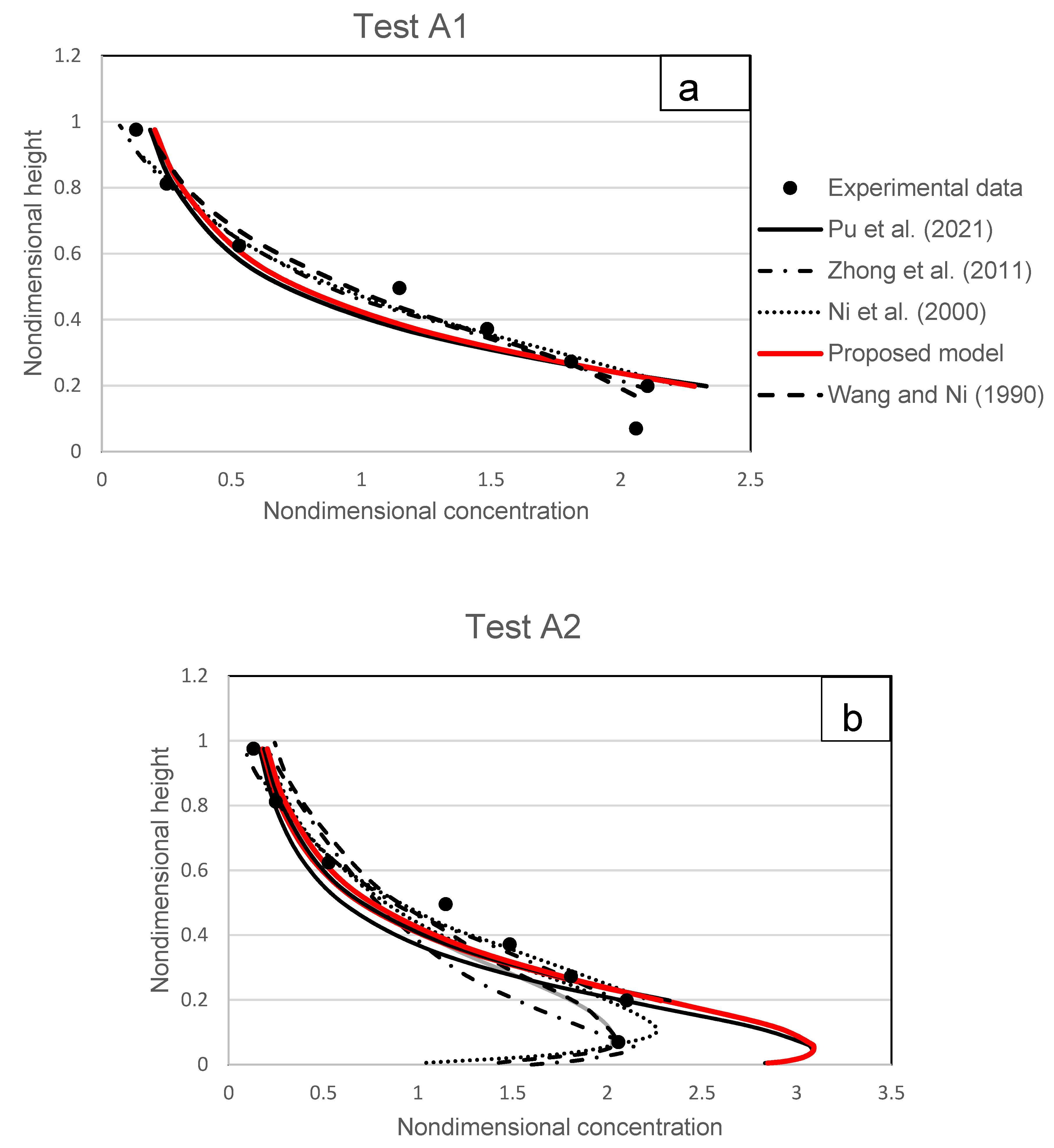
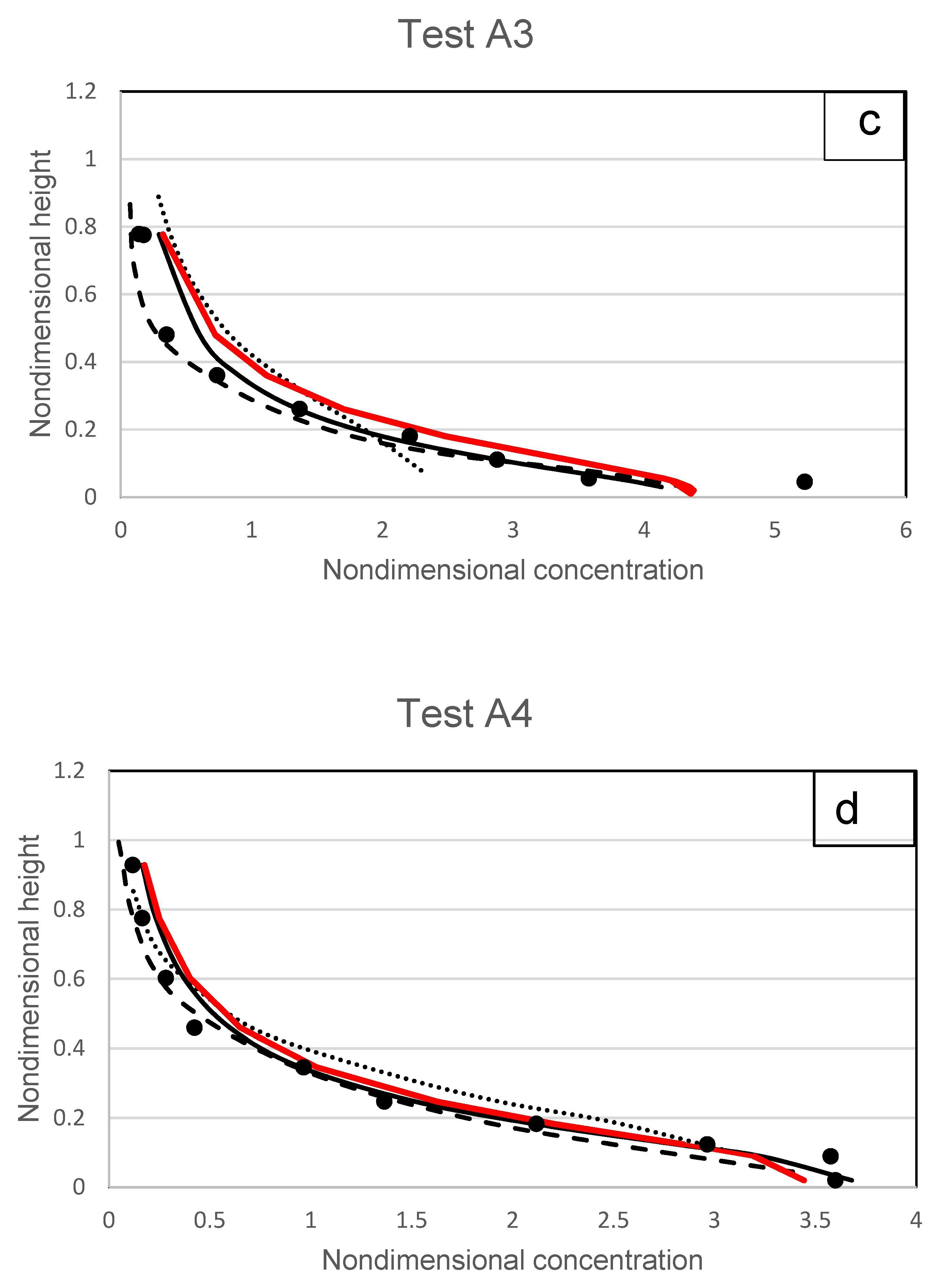
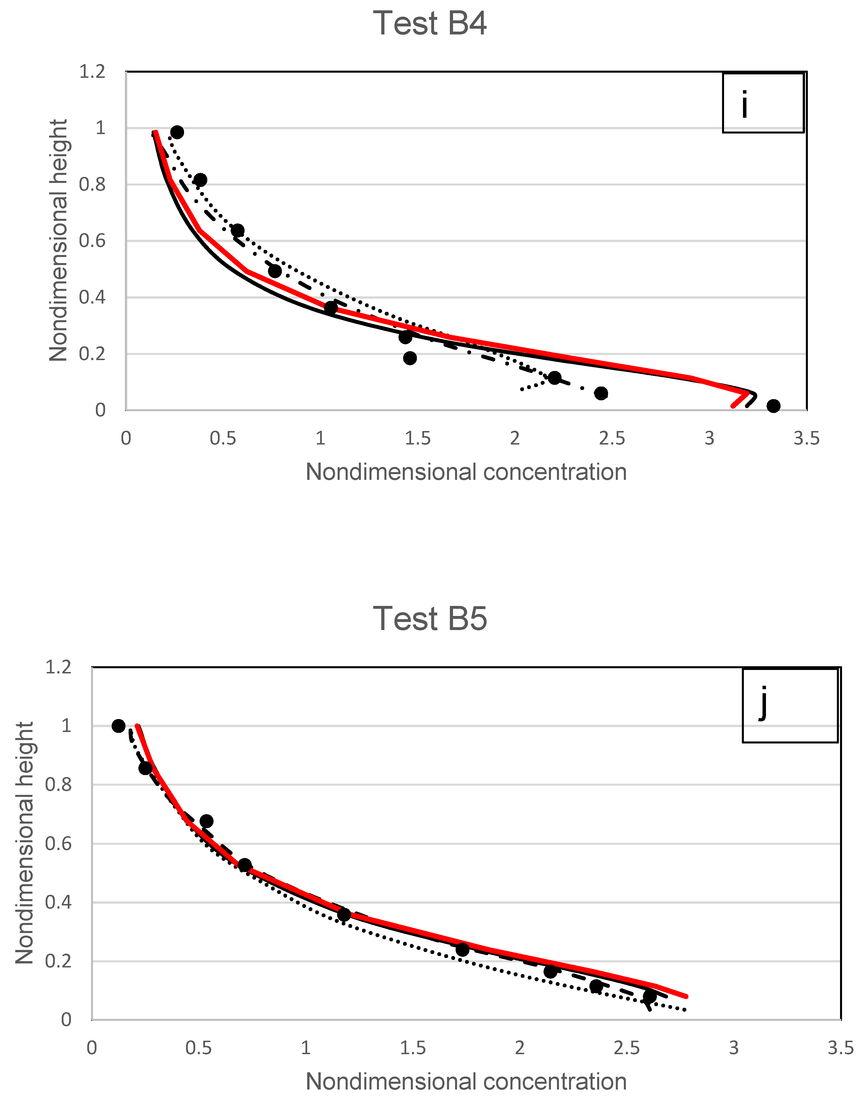
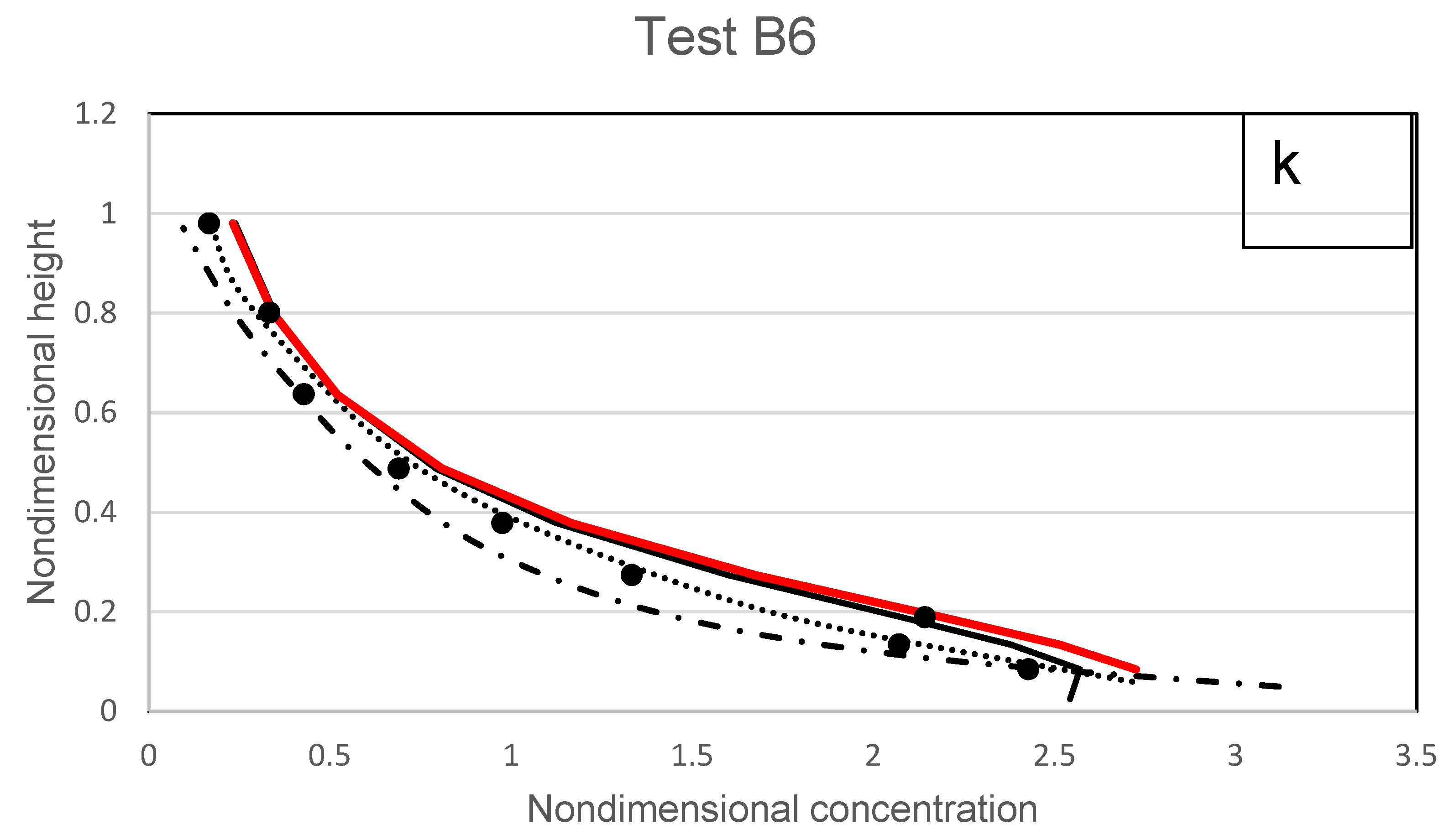
Figure 17a–k. The measurements of Wang and Ni [
31] show that for diluted flow the sediment concentration tends to follow the type I or II profile where the maximum concentration occurs at the near-bed region.
The results shown in
Figure 17a–k demonstrate that overall, there is a better fit between the proposed models and other models away from the near-bed regions. The proposed model corresponds to the experimental data well in the middle and free surface regions. In cases A1, A2, A6, A7, B3, and B4, the proposed model predicts experimental data better than the model proposed by Pu et al. [
1] and other models. This is consistent with the literature [
1,
4,
8] which states that possibility of particle–particle collisions increases near-bed to produce conditions that are more challenging to represent with mathematical modelling.
The biggest particles among all the measured data from Wang and Ni [
31] were used in the experimental data presented in
Figure 17g. Due to the higher surface area of the sediment particles, there would be stronger forces coming from the solid–fluid phase interaction. One can see that the concentration distribution for A7 shown by the proposed model (
Figure 17g) is consistent with the observations. The suggested model exhibits the promising computation of big particles in observed data when compared to a model such as those by Zhong et al. [
23] that does not account for particle size. In addition, the tests A5 and B5 are the smallest particle diameters, and the proposed model is doing better than Ni et al. [
10] which relies on empirical particle interactions.
4.2. Wang and Qian
Using an experimental recirculating-tilting flume, Wang and Qian [
37] investigated the impact of diluted to dense concentrations in an open channel flow. Their tests included silt with diameters ranging from 0.15 mm to 0.96 mm and concentrations ranging from 0.0102 to 0.0906. All the conditions tested are shown in
Table 4. As a result, their tests have been used in this comparison with the suggested and other earlier models as the findings shown in
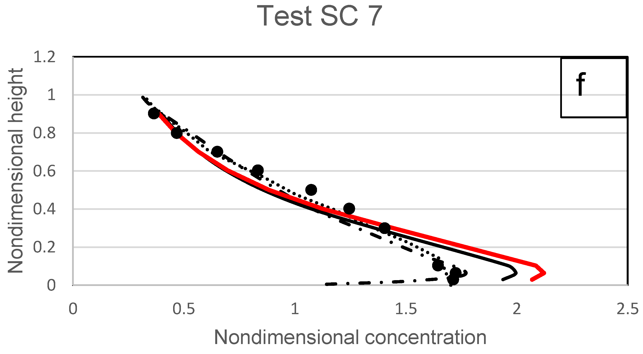
Figure 18a–f. In general, the models’ accuracy declines as the mean concentration rises across the flow depth. In particular, in the upper-flow zone, the experimental data are reasonably fit by the suggested model. The lift and drag caused by the fluid-induced forces as well as the inertia of the sediment particles are the principal forces acting on the particles in the upper layer. This demonstrates that the proposed model’s incorporation of the Rouse and size parameters allows it to accurately calculate the solid-fluid interactions for individual particles.
The accuracy of the various models, including the suggested model, decreases at the lower-suspension region, according to an overview of all the results shown in
Figure 18. Compared to type III profiles, type II profiles have higher concentrations and a smaller turning point near the bed. Rather than suspended load, bedload behaviour governs the distribution of sediment along the wall boundary. In Wang and Qian’s [
37] investigation, plastic particles were also utilised in the flow, and theoretically, under the influence of particle–particle interacting forces, it produced less notable movement than the normal and natural sediment. This means that, in contrast to models by Ni et al. [
10] and Zhong et al. [
23], which incorporated empirical functions discovered from the relevant experiments into the modelling, the proposed model, which deals with the forces by coupling expressions of Rouse and size parameters, is unable to simulate its near-bed concentration reasonably for experiments SF2, SC5, and SC6 as shown in
Figure 18a,
Figure 18e, and
Figure 18f respectively. Results of the proposed model are better than those from Pu et al. [
1] for experiments SF5, SM6, and SM7 as shown in
Figure 18b,
Figure 18c, and
Figure 18e.
4.3. Michalik
Michalik [
36] researched the sediment profile of hyper-concentrated flows using experimental data. Sand with a diameter of 0.45 mm and concentrations ranging from 0.15 to 0.54 was employed as the sediment material (all the tested conditions are shown in
Table 5). The linear law found in Equation (20) is used in this study to model Michalik’s tests. The test findings are displayed in
Figure 19a–h, where measurements and the proposed model results are contrasted.
The sediment-concentration distribution from the investigated hyper-concentrated flows displays a type III characteristic. It is challenging to precisely calculate the concentration distribution’s turning point in a hyper-concentrated flow. This is due to the fact that the boundary between the sediment’s bed and suspended states is not clearly defined, but rather, the bedload will diffuse into the suspended state through a transitional zone. Because of this, the suspended load has occasionally been calculated as a portion of the bedload, which widens the gap between measurements and suspended sediment modelling. A correct assumption of
and
is necessary in order to precisely describe the transition zone and, consequently, the position of the turning point [
29]. Given that both the variables are constant in this study’s proposed model and are not changing in an experiment, it is reasonable to draw the conclusion of
and
[
38].
The suggested model shows a decent fit of the type III profile to the hyper-concentrated distribution and offers a reasonable match to the experimental data. As demonstrated in Michalik [
36], studies of hyper-concentrated flow demonstrate that as
increases, the sediment concentration distribution becomes more homogeneous. Power distributions may not be appropriate to model hyper-concentrated flow as a result. Rather, a linear model is used here, which has been shown to generate superior accuracy.
The height of the maximum concentration also increases as the mean concentration rises, possibly as a result of the growing possibility of a bedload layer close to the bed. The near-bed region becomes increasingly saturated as the mean concentration rises. The experiments in
Figure 19 demonstrate that the settling velocity has no effect when
0.31 and that the dominant interaction forces must result from particle–particle reactions. The suggested model accurately depicts the concentration distribution in these highly concentrated tests of
0.31. In particular, for the majority of cases, the suggested model correctly predicts the height at which the greatest concentration (turning point) occurs.
5. Conclusions
For accurately estimating the diluted and hyper-concentrated distributions over typical heights within the flow, a parameterized power-linear coupled model with machine learning has been validated. The machine learning models used were XGboost Classifier, Linear Regressor (Ridge), Linear Regressor (Bayesian), K Nearest Neighbours, Decision Tree Regressor and Support Vector Machines (Regressor). The models were implemented using Google Colab. The models have been applied to investigate the relationship between every Kundu and Ghoshal [
4] parameter with each sediment flow parameter namely, mean concentration, Rouse number, and size parameter. The distribution of suspended sediment over the characteristic height inside the flow was inclusively estimated from diluted to hyper-concentrated. Comparisons with experimental data from Wang and Ni [
31] on highly diluted flows, Wang and Qian [
37] on mixed diluted to dense flows, and Michalik [
36] on hyper-concentrated flows for low and extremely high concentration testing that approximates type I to III profiles, the proposed power-law and linear-law models are more precise than Pu et al. [
1] in some cases, and in other cases, just as precise as those of Pu et al. [
1]. Finally, it is shown that the models produced from machine learning are capable of calculating the suspended sediment profile accurately under a variety of flow circumstances (
), including different Rouse numbers (
).

 and
and 


