1. Introduction
In this paper, we develop a numerical approach to the simulation of three-dimensional incompressible multiphase flows involving multiple fluid phases as well as solid inclusions or boundaries of arbitrary shapes. The proposed algorithm is implemented in the open-source environment Basilisk [
1] and is validated on several fluid dynamics problems demonstrating its capabilities for solving challenging multiphase multiscale flow problems.
Multiphase flows are of importance to many areas of applied science and engineering. Sprays and jets from nozzles are a common occurrence in mechanical, chemical, and aerospace engineering [
2,
3,
4,
5]. Chemically reacting flows in multiphase systems are important for combustion applications [
6], microreactors [
7], and energy storage technologies [
8,
9]. The motion of bubbles, droplets, and particles in viscous flows are important in the oil and gas industry [
10,
11,
12], biology, and medicine [
13,
14,
15,
16,
17]. The design of microfluidic devices requires the understanding of multiphase flows in small channels of complex shapes [
14,
18,
19,
20,
21]. Numerous manufacturing applications also relate to multiphase flows involving, for example, the formation of bubbles during composite manufacturing [
22]. Detailed numerical simulation in problems involving multiphase flows is associated with extra challenges compared to single-phase flows due to the need to accurately resolve various features associated with interfaces, which often requires sophisticated algorithms and, in the presence of multiscale dynamics, substantial computational resources [
21,
23]. The reader can find general and extensive discussions of the theory, computational techniques, and applications of multiphase flows in recent and classical books, such as [
23,
24,
25,
26,
27,
28].
In multiphase flows, the fluid–fluid interface is generally a dynamic unknown surface that is to be determined as part of the solution. One can describe such flows by writing governing systems of equations for each fluid region separated by the interface and supplementing them by kinematic and dynamic interface conditions. Such equations coupled via the interface conditions can then be discretized and solved numerically. This direct approach is generally quite challenging to implement as it requires one to track the evolution of the interface and to carefully handle topological changes associated with the break-up or merger of domains with different fluids.
The present work uses a different formulation that provides a simple and efficient way to handle problems with the interface identification. The formulation is based on the introduction of a scalar field that serves as an indicator function for each fluid phase and allows one to track the interface motion by solving an appropriate evolution equation for the function. For example, one can define function
that has a value pf 1 in the first fluid and a value of 0 in the second fluid, or
could have different signs on different sides of the interface and be zero on the interface. Many methods based on such ideas have been designed to solve for the interface evolution, including the front tracking method [
29,
30,
31], the boundary integral method [
32], the phase field method [
33,
34], the volume of fluid method (VOF) [
35,
36], and the level set method [
37,
38].
Our formulation is based on the VOF method, which was originally proposed by Hirt and Nichols in 1981 [
35] and has subsequently been improved in many works, for example [
39,
40,
41]. There exist two versions of the method: the geometric VOF [
41,
42] wherein the distribution of
is found geometrically by, e.g., advecting a plane interface with a predefined velocity
, and the algebraic VOF [
43] wherein
is represented by a function, such as a polynomial or trigonometric function. The geometric VOF is more widely used due to its advantages in terms of mass conservation, robustness to topological changes, such as a merger or break-up, and relative ease of extension to high dimensional Cartesian grids [
44]. However, it should be noted that the geometric VOF method is harder to implement in parallel.
The surface tension of a fluid interface is treated by the so-called “continuum surface force” (CSF) model, originally proposed by Brackbill et al. [
45]. In this model, the surface tension is represented as a body force highly concentrated in the vicinity of the interface. Other related models can be found in the literature [
46,
47]. The CSF model is easily coupled with various fixed (Eulerian) mesh formulations for interfacial flows, in particular with the VOF [
45,
48], level set [
49,
50], and front-tracking methods [
3,
30,
51]. Recent improvements of CSF are associated with the reduction of spurious currents using the balanced force algorithm [
46,
52] and with improving the interface curvature evaluation [
53,
54]. We also mention a related continuum surface stress method [
55,
56,
57] that represents the surface tension as the divergence of the capillary pressure tensor. The main advantage of this method over CSF is that it naturally takes into account tangential stresses, such as Marangoni stresses (which are not considered in the present work).
The presence of solids in multiphase flows is associated with many computational challenges especially if the solids are of a complex shape and are not stationary. When considering only mesh-based schemes for such multiphase flows, there are two approaches to represent the geometry of the solids: (1) based on body-fitted methods, wherein the mesh boundary is aligned with the surface of the solids or (2) the immersed boundary (IB) methods, wherein the boundary conditions are incorporated in the governing equations, and the solid region becomes part of the computational domain. The first of these options allows for an easy formulation of the boundary conditions. However, when bodies experience large deformations or move fast, a grid has to be reconstructed frequently, which leads to large overhead. Moreover, during the frequent reconstructions, one must avoid the appearance of geometrical singularities and small angles in order to obtain high-quality meshes. Although the automatic generation of body-fitted grids has been developed [
58,
59], the task remains challenging and labor-intensive [
60], especially when bodies move. Such methods are also difficult to generalize to high-order schemes, so most body-fitted methods are low-order.
In contrast, the IB methods [
61] allow for high-order schemes, arbitrary geometries, and moving solids. The first IB method was proposed by Peskin in 1977 [
62] to simulate the interaction of cardiac mechanics and blood flow. The main feature of the method is a non-body conformal Cartesian grid in which a new approach is formulated to consider the effects of the immersed boundary on the flow. Specifically, the fluid is modeled on a fixed Cartesian grid, but the boundary is modeled on a curvilinear Lagrangian mesh, which moves freely across the fixed mesh. In this technique, a grid is not body-fitted. The immersed boundary is provided by an additional surface grid that cuts across the Cartesian grid. The non-conformity of the wall and the grid leads to the modification of the Navier–Stokes equations [
63] by incorporating an artificial force term that models the effects of the boundary in such a way that guarantees boundary conditions by slightly adjusting the fluid velocity field near the solid surface using various kernel functions [
61].
One of the IB methods is the Brinkman penalization method (BPM), which was originally developed by Arquis and Caltagirone [
64] for the numerical simulation of isothermal obstacles in incompressible single-phase flows. The general idea of the BPM is based on the work of Brinkman [
65] in which solids are considered porous media with very small permeability,
, and fluids as media with large permeability,
. In BPM, the permeability is taken as a penalization parameter. One of the advantages of BPM is the availability of a convergence proof and error estimates depending on the penalization parameter, which have been thoroughly studied by Angot et al. [
66]. Furthermore, the enforcement of boundary conditions on the solid requires no modifications to a numerical scheme near the solid surfaces. It is therefore relatively easy to design an efficient and robust parallel code [
67].
In the present work, interfaces are tracked by the VOF method [
39], and solids are considered by BPM. The algorithm is implemented in the open-source software Basilisk [
1], which uses efficient adaptive meshes. The BPM and VOF methods can be implemented for fixed or adaptive grids. The adaptive mesh refinement reveals the best capabilities of the BPM and VOF methods when the mesh compression ratio (the actual number of cells relative to the number of cells at maximum refinement) is larger than
[
68].
In [
69,
70], the authors also consider coupling of VOF and BPM. In [
69], non-zero contact angles on the surface of stationary solids are analyzed using fixed meshes, while in [
70], the solids are treated with adaptive Cartesian meshes under perfectly wetting conditions. Our work considers fixed as well as moving solids using adaptive meshes; perfectly wetting and perfectly non-wetting surfaces are assumed.
The remainder of the manuscript is organized as follows. In
Section 2, we introduce the governing equations together with the main ideas behind the numerical approach. The detailed description of the numerical algorithm is presented in
Section 3. In
Section 4, we discuss a number of simulation results, including validation tests of the method by solving several multiphase flow problems. Conclusions are presented in
Section 5.
2. Governing Equations
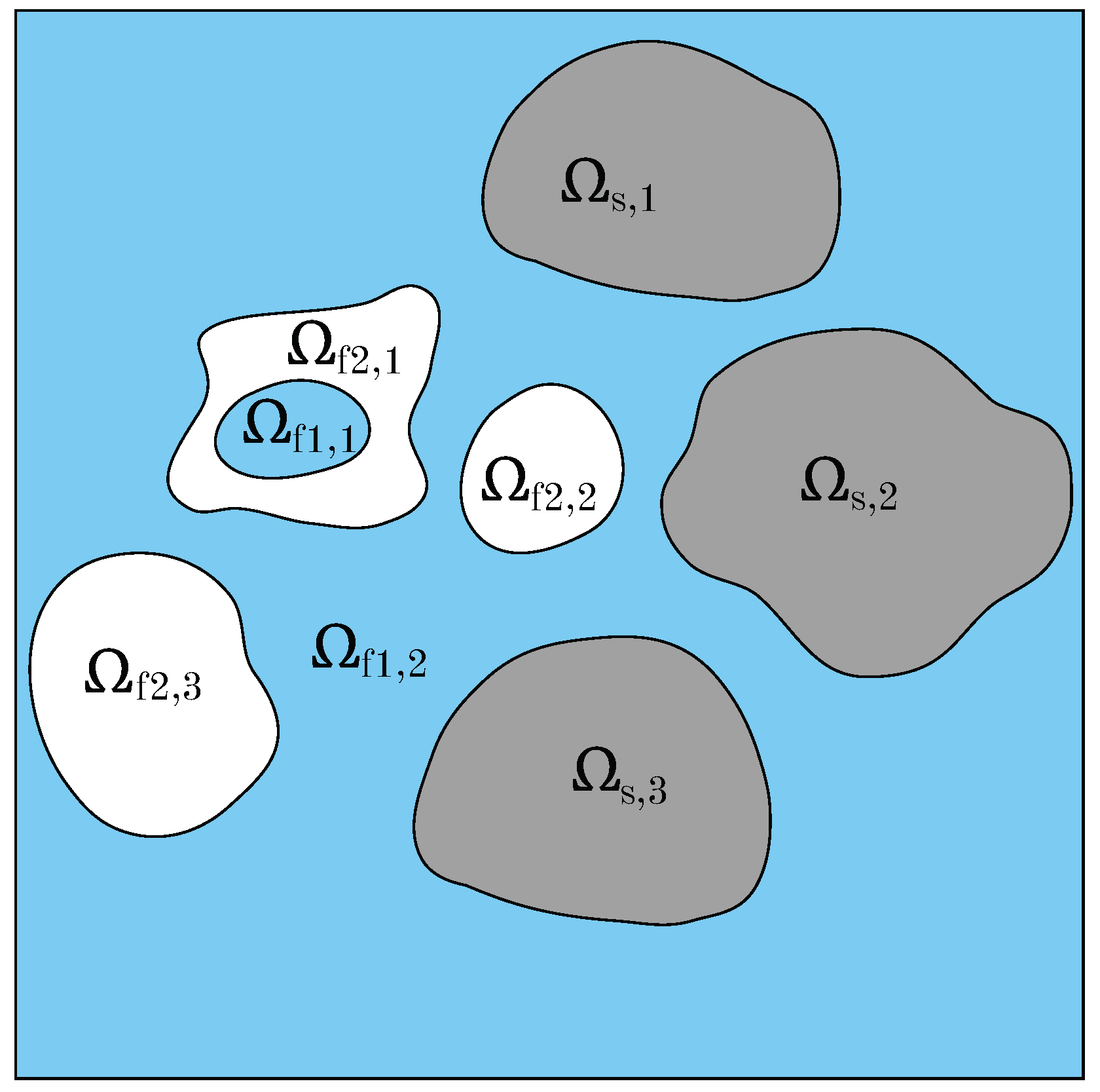
The governing equations are based on the Navier–Stokes equations for incompressible Newtonian fluids adapted to treat multiphase flows in a system with complex topology involving multiple fluids and solid inclusions. The solids are assumed to move with a prescribed velocity. The solid surface is considered to be either perfectly superhydrophilic or perfectly superhydrophobic.
The computational domain
is assumed to contain two fluids in subdomains
,
, and stationary or moving solids in subdomains
. Each subdomain can be a multiply connected region with an arbitrary shape, as illustrated in
Figure 1. The fluids are assumed to be immiscible and to have different densities
and viscosities
,
. The no-slip boundary condition is set on the surface of solids such that
where the solid velocity field
is assumed prescribed.
The Navier–Stokes equations for multiphase flow can be reformulated as a single system for the velocity field
in the whole domain. The effect of surface tension is then included in the momentum equation as a volumetric force
concentrated on the fluid interfaces. The presence of solids is captured by the penalization force
[
66,
71] that acts inside solids and also enables imposing the boundary condition (
1). Then, the fluid motion is governed by the continuity and modified Navier–Stokes equations:
where
p is pressure,
is the viscous stress tensor, and
is the gravitational acceleration. The local average density
and dynamic viscosity
of the fluids are calculated via the local volume fraction
of fluid 1 using a linear interpolation:
where subscripts 1 and 2 refer to the primary and secondary fluid phases. The parameters
are assumed constant. The volume fraction
is governed by the advection equation
2.1. Surface Tension Force
The surface tension force is incorporated into the momentum Equation (
3) as a source term
that is highly concentrated in the vicinity of the interface. This continuum surface force (CSF) approach was proposed in [
45] and is widely used for the simulation of flows with free interfaces. The main advantage of the CSF is the one-shot calculation throughout the computational domain and the relatively straightforward implementation. The surface tension force
in Equation (
3) is given by:
where
is the average density of the two fluid phases,
is the coefficient of surface tension, and
is the total curvature of the interface obtained using
, where
is the unit normal to the interface.
To model perfectly non-wetting (perfectly superhydrophobic) or perfectly wetting (perfectly superhydrophilic) surfaces, the volume fraction of fluid 1 inside solids is given by:
2.2. The Penalization Term
The presence of the solid phase is reflected in the modified Navier–Stokes equation by the Brinkman penalization term
, and the approach is called the Brinkman penalization method (BPM) [
66,
72]. The method considers solids as porous media with a vanishing permeability. The source term
in the governing equations enforces the desired velocity
inside the solids.
For the Dirichlet boundary condition from Equation (
1), the term
in Equation (
3) is set as
where
is a penalization coefficient having the dimension of time, and factor
is a mask field defined as
Angot et al. [
66] theoretically proved that as
, solutions of the penalized Equations (
2) and (
3) converge to the solutions of the original Navier–Stokes equations with correct boundary conditions. The upper bound on the global errors of the normal and tangential components of velocity were shown to satisfy the estimates
where
and
are constants that depend only on the problem setting. These estimates indicate that the normal component of the velocity converges to the target value faster than the tangential one. Note, however, that even though taking smaller values of
gives better results, there is a practical limitation of the method associated with the presence of discretization errors. As we show in
Section 4.2, the error
reaches a plateau when
. The error is seen to decrease as
tends to 0 until the viscous and penalization terms become of the same order of the magnitude inside the solid, i.e.,
. After that, the plateau is reached (see Figure 8). In terms of the characteristic velocity
and thickness
, the size of the Brinkman layer can be estimated from the balance
that gives
. This size must be resolved numerically with at least
mesh cells [
71,
73]. To ensure this, one can take the penalization coefficient as
The BPM requires a specification of viscosity and density in the whole domain, even inside solids. The density
of the solid can be taken as a real physical value, but the viscosity of the solid,
, has no physical meaning. Nevertheless, it was observed in numerical experiments that taking large values of
improves the efficiency of computations. Here,
was chosen (somewhat arbitrarily), assuming that the kinematic viscosities of the primary heavy fluid (fluid 1) and the solid are the same, which makes the kinematic viscosities continuous across the fluid–solid interface:
. Note that taking a
value that is too small leads to a slow convergence of the solution. One should also avoid taking a
too large. Either way, the average viscosity and density are found from
These definitions ensure that: inside solids ( and any ); inside fluid 1 ( and ); and inside fluid 2 ( and ).
3. Computational Algorithms
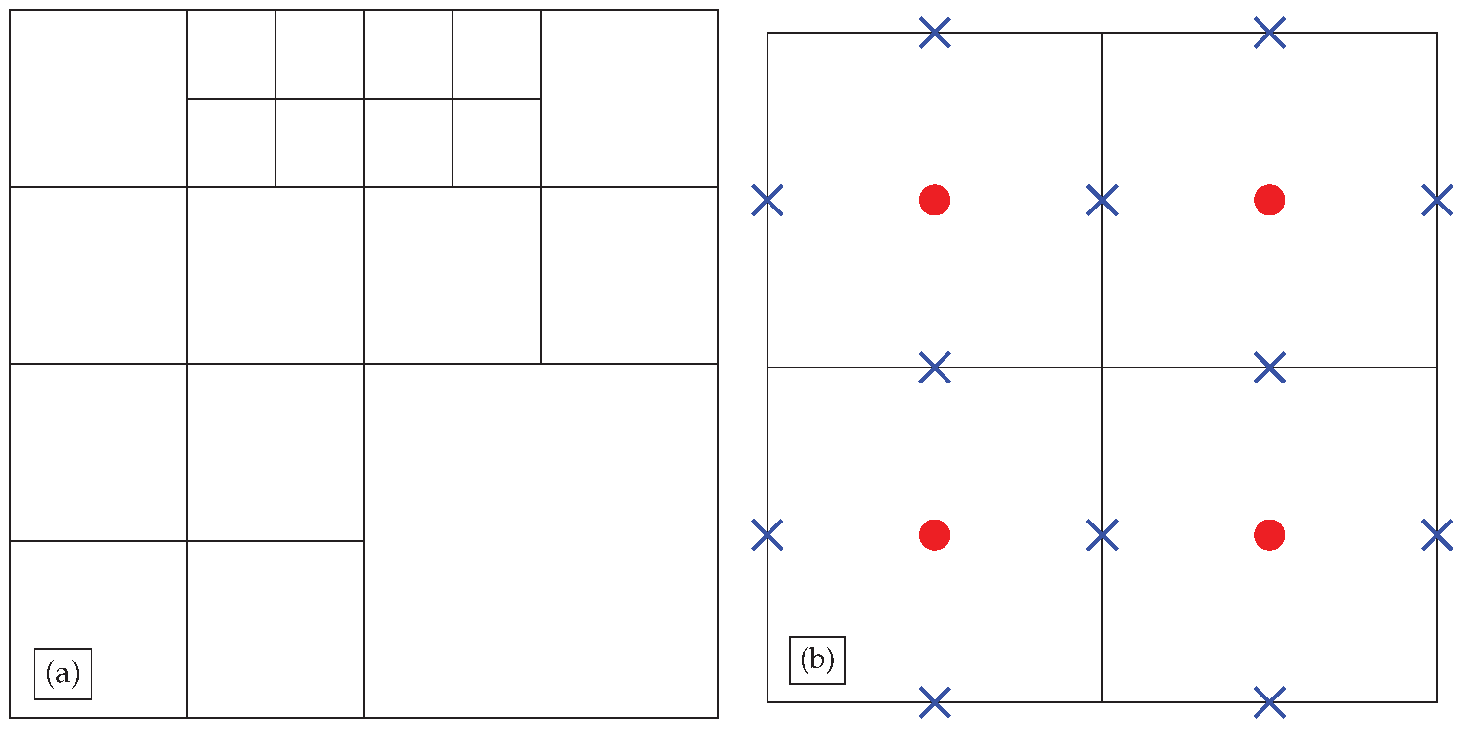
The computational domain
is spatially discretized using square (cubic in 3D) finite volumes forming a hierarchical structure; the so-called quadtree (octree in 3D) [
74] is schematically shown in
Figure 2a. Variables are defined either at the cell centers or on their faces, as shown in
Figure 2b. The incompressible Navier–Stokes solver in Basilisk uses a standard staggered grid, where the pressure
p is specified only at the cell center, but the velocity is specified both at the cell centers as
and the centers of the cell faces as
. Similarly, the solid volume fractions are specified at the cell centers as
and at the face centers as
. Both
and
are determined using the distance functions at the vertices. The density
and volume fraction
of fluid 1 are also defined at the cell centers, while viscosity
, acceleration
, and specific volume
are defined at the cell faces, where
is computed using Equation (13), and the face-centered value
is linearly interpolated using two adjacent cells.
We develop the numerical algorithm for the solution of the main governing system by splitting various physical processes and treating them separately either explicitly or implicitly. The algorithm consists of six main steps, which are explained in detail below: (1) the volume of fluid step, in which the volume fraction
is updated; (2) the advection step for momentum in Equation (
3), in which the velocity field
is updated using the Bell–Colella–Glaz scheme [
75]; (3) the implicit update of the viscous and Brinkman penalization terms as well as of
; (4) the updates of the surface tension and gravity terms together with the face velocity
; (5) the Chorin projection step is taken [
76], in which the incompressibility condition is imposed and the pressure field
p is found; and (6) the mesh adaptation step, where the mesh is refined in the regions with large gradients or coarsened in smooth regions.
3.1. Step 1: Volume of Fluid (VOF)
The VOF is a sharp interface method that evolves fluid interfaces using the tracer field
satisfying the advection (Equation (
5)). When advecting
from the time level
to
using a conservative, non-diffusive geometric VOF method [
39,
42], we obtain:
where
is the corrected velocity field defined on the cell faces. The face-velocity correction is required in order to adjust the flow so that the fluid does not penetrate into the solid by more than two cells. We use the following correction of
to obtain
:
where
is the solid velocity obtained by averaging the cell-centered velocity
, and
is the face-centered indicator function computed from the face-centered solid volume fraction
. The indicator function
is 1 inside the pure fluid domain (
), and 0 even if the cell contains a small volume of the solid body (
). Such a formulation does not strictly respect the mass conservation. Nevertheless, in the verification tests in
Section 4.3 and
Section 4.4, we demonstrate that the mass loss is negligible (<
for fine mesh and <
for coarse mesh). In the first time step,
is taken as the average value of the cell-centered velocity
. In the multi-dimensional VOF advection scheme, the field
is advected along each dimension in series using a 1-D scheme.
The VOF method allows one to simulate multiphase flows with complex topological changes using sharp interface representation. However, its implementation is not without challenges. It requires an accurate calculation of the interface normal and the curvature, which involves calculating second derivatives in space (see subsequent steps of the algorithm below). One may face numerical artifacts, such as discretization-induced flow, and hence the absence of convergence with grid refinement [
53,
56]. Consequently, most approaches do not estimate the curvature directly from the VOF function but instead use a smoothed VOF function via convolution, discrete quadrature [
77], and others.
One approach to addressing these problems is based on the construction of a height function
H for the calculation of interface normals and curvatures [
53]. For each interface cell, fluid “heights” are calculated by summing the fluid volume in the direction of the largest normal component
,
, or
. This summation is performed on a
stencil around all interface cells with the size
h. Note that in 2D,
H is a vector, and in 3D,
H is a tensor. For example, if for some interface cell the largest normal is directed along
z, then the height
H for a cell
can be found from
The curvature
and the gradient
in Equation (
6) are then calculated as:
where
, and the nabla operators with
indices indicate the divergence or gradient only along the indicated directions.
When the HF stencil crosses a highly curved interface more than once, the standard height-function method stops working. Then the HF method is locally switched to the parabola-fitted curvature method [
52]. The idea behind this method is to fit the interface points with a parabola in 2D and a paraboloid in 3D and differentiating the resulting analytical function to estimate the curvature.
3.2. Step 2: Advection
At this stage, the Bell–Colella–Glaz (BCG) scheme [
75] is applied, which is second-order in time and space. The viscous and Brinkman penalization terms from Equation (
8) are omitted. For simplicity, the method is described here for the two-dimensional case.
Let and . The BCG method estimates the face velocity at the half time step and then advects the cell-centered velocity field as a passive tracer. The face velocity in the intermediate timestep is extrapolated along characteristics using the cell velocity and the term . The velocity and auxiliary fields at the faces are estimated by averaging the left and right neighbors for their x components and, correspondingly, bottom and top neighbors for their y components. Such averages are denoted by an overbar: .
Thus, the face velocity
at the intermediate temporal layer
for the
x component is given by
where
h is the cell size,
is the CFL number,
is responsible for the direction of the flux, and the index
S denotes which neighboring variable is used. Since this extrapolation does not guarantee incompressibility, the Chorin projection step is taken (see
Section 3.5), which subtracts the non-solenoidal component from the velocity field
and gives the velocity at the half step
. The
x component of the velocity
is updated as:
where the index
a indicates advection,
,
are fluxes along direction
d, with
indicating right or top face values and
left or bottom face values. For example,
can be obtained by a procedure similar to Equation (
18):
where
is the CFL number,
is a direction, and
is averaged from face values as
.
The sum of the pressure gradient, surface tension, and body acceleration, i.e.,
, is used in the calculation of cell-centered variable
as follows:
Note, that in Equation (
20),
is used for more accurate computation of fluxes at cell faces.
The explicit integration gives a restriction on the time step: , .
3.3. Step 3: Viscous Force and Brinkman Penalization
At this step, we solve the momentum equation with only the viscous and Brinkman penalization terms. Since the stiff viscous term imposes a strong time-step limitation (
), and the Brinkman penalization term is also stiff, these two terms are integrated with an implicit scheme as follows:
where
is the cell-centered velocity, the penalization coefficient
is computed by Equation (
11), and
is the cell-centered volume fraction of solids. The density
and viscosities
are computed using Equations (
12) and (13), in which instead of the volume fraction
, the smoothed volume fraction
is used. The smoothing is done by linearly interpolating values from the nearest cell-centered neighbors. The viscous term has the standard second order central-difference discretization in space. A similar equation without contribution of
is solved by the multigrid method with Jacobi iterations in [
78,
79].
3.4. Step 4: Surface Tension and Gravity
The cell-centered velocity is based on an old value of , which is computed from the sum of body acceleration , surface tension acceleration , and the pressure gradient on the old time layer n. The following steps update the field in order to then subtract the old : and then add the new . Therefore, we first update all accelerations and calculate the face velocity interpolating between neighboring cells and adding the new acceleration: . The resultant velocity field is not solenoidal, and therefore, the Chorin projection is applied (the next step).
3.5. Step 5: Chorin Projection
The velocity and pressure fields are strongly coupled. The direct integration of Equation (
3) does not guarantee the incompressibility of the fluids; that is, the interpolated
derived from
does not satisfy the incompressibility condition. To obtain a divergence-free velocity field
, the Chorin projection step is used [
76]. It is based on the Helmholtz decomposition whereby the velocity vector field is split into a solenoidal (
) and a curl-free (
) components. The projection begins with solving the pressure Poisson equation
Subsequently, the non-solenoidal part of the velocity is subtracted as
This guarantees that up to a given threshold in the Poisson equation. After the computation of a new pressure field , it becomes possible to compute , first on the faces, then in the centers of the cells using interpolation. Finally, is computed as .
The last step of the integration cycle is the grid adaptation [
74,
80] based on, for example, the volume fraction
of fluid 1, volume fraction
of the solid, or velocity
. The grid is refined or coarsened following the standard wavelet-based adaptation criterion [
81].
One final note of this section concerns the choice of the integration time step. There are two limiting factors in the time step
: the convection with the maximum flow velocity
, which comes from the advection in Equation (
5), and the capillary waves with the capillary phase speed
[
45,
82], where
, and
k is the wavenumber. The maximum possible wavenumber in a finite difference scheme is
, which corresponds to the minimum wavelength
. Hence, the time step is chosen from the minimum estimates:
Summarizing the steps above, we have the following final algorithm.
We note here that steps 3 and 12 of Algorithm 1 are new and have previously not been implemented in Basilisk. Step 3 addresses the problem of fluid penetration into the solid, and step 12 accounts for the presence of solids implicitly (in numerical integration) rather than explicitly as in SSM.
| Algorithm 1 The algorithm of multiphase modeling in Basilisk |
Require: Set initial and boundary conditions for , , , and . Notation: . - 1:
while (time integration loop) do - 2:
Set time step based on the CFL condition and surface tension restriction (Equation ( 25)). - 3:
Correct face velocity . - 4:
Find volume fraction using the VOF method in Equation ( 14). - 5:
Calculate fluid properties , and from using Equations (13) and (12). - 6:
advection step: - 7:
Predict using Equation ( 18). - 8:
Correct to obtain divergence free (Chorin’s projection in Equations (23) and (24)). - 9:
Calculate using the Bell–Colella–Glaz scheme (Equation ( 19)). - 10:
viscous step: - 11:
Calculate . - 12:
BPM: find based on using Equation ( 22). - 13:
Calculate . - 14:
Calculate acceleration using Equation ( 6) and velocity . - 15:
Correct to obtain divergence free and pressure (Chorin’s projection in Equations (23) and (24)). - 16:
Calculate on faces and then interpolate to cells . - 17:
Update using the new acceleration and pressure . - 18:
Adapt mesh. - 19:
end while
|
4. Numerical Simulations
In this section, we present the results of several simulations that are used to assess the validity and accuracy of the proposed algorithm. First, we model the two-dimensional Stokes flow of a single-phase fluid past a periodic array of identical cylinders. We investigate the convergence of the drag force to the theoretical solution and also compare the BPM with several other numerical methods. Second, we study the decaying vortex problem for which an analytical solution exists. Third is a multiphase case, in which we investigate the multiphase flow of a bulk viscous fluid with embedded droplets of a different fluid past a periodic array of cylinders. This problem has no analytical solution and is used for the purpose of verifying mass conservation. Fourth is the case involving a moving solid. We demonstrate the robustness of the proposed method with a situation in which a cylindrical solid covered with a layer of one viscous fluid starts moving inside another viscous fluid, which, at some point, ruptures the layer covering the solid. We have also verified that the algorithm satisfies the Galilean invariance by simulating the motion of a cylinder or a sphere along the interface between two fluids.
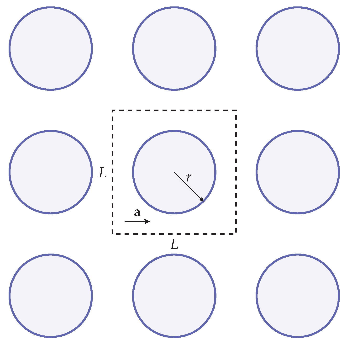
4.1. Viscous Flow Past a Periodic Array of Cylinders
Here, we solve numerically a problem that was studied theoretically in [
83]. Consider an infinite square array of cylinders of radius
r immersed in an incompressible viscous fluid with density
and viscosity
. The cylinders are assumed stationary. The spacing between them is measured by the distance
L between the centers of the nearest neighbor cylinders. Since the system is periodic, we consider a square box with size
L, as shown in
Figure 3. Then the distance between the surfaces of the adjacent cylinders is
, and the solid volume fraction is equal to
. The fluid motion is assumed to begin from rest under a uniform body force
directed from left to right. The fluid flow reaches a steady state when the drag force becomes equal to the body force. The mean flow velocity in the
x direction is denoted by
. We assume that the Reynolds number
is small so that the Stokes flow approximation holds.
The steady-state problem was solved in [
83], and we compare our simulation results to that work. In [
83], the authors solved the creeping flow equations with the no-slip condition at the surface of the solids and periodic boundary conditions. They obtained an approximate solution and used it to calculate the dimensionless drag force
f on a cylinder as
where
F is the drag force per unit length,
p is the pressure,
is the vorticity, and the integration is taken over the cylinder boundary with polar angle
. This force
f strongly depends on the solid volume fraction
, increasing with the radius of the cylinders, and it was shown to be given by
where
and
are certain coefficients from the series expansion of the solution, which are obtained numerically and which depend on
. Asymptotic solutions for two extreme cases can be explicitly derived for: (i) dilute arrays
and (ii) concentrated arrays
:
where
is the volume fraction of the particles when the cylinders touch each other.
Values of
f for different solid fractions are listed in
Table 1. In the same table, we compare the relative error
in drag force obtained by the Brinkman penalization method with two other methods: the simple splitting method (SSM) and the embedded boundary method (EBM), both available in Basilisk software. Here,
is the force computed from the numerical simulations. In the simple splitting method (SSM) [
84,
85], the
cell-centered velocity update is given by
, where
is the velocity field calculated without accounting for the presence of solids. In the embedded boundary method (EBM) [
86,
87], the auxiliary forcing term is not explicitly computed as in the IB methods, but instead, the values of the state vector inside the solid body are set so that the fluxes through the solid surface vanish.
The simulation results are compared with the predictions of [
83] in
Table 1. The grid with
is used, and the penalization coefficient is
. Since the dimensionless drag force
f has a singularity when
tends to
, the numerical error
E grows with the increasing
. The SSM shows poor convergence, especially for the narrow-gap cases, and the discrepancy between the analytical and numerical solutions diverges rapidly. The EBM is in good agreement over a wide range of porosity. The BPM is seen to have better accuracy at
. Overall, the EBM and BPM are comparable in their accuracy in this case. However, the BPM is easier to extend to multiphase flow problems than EBM.
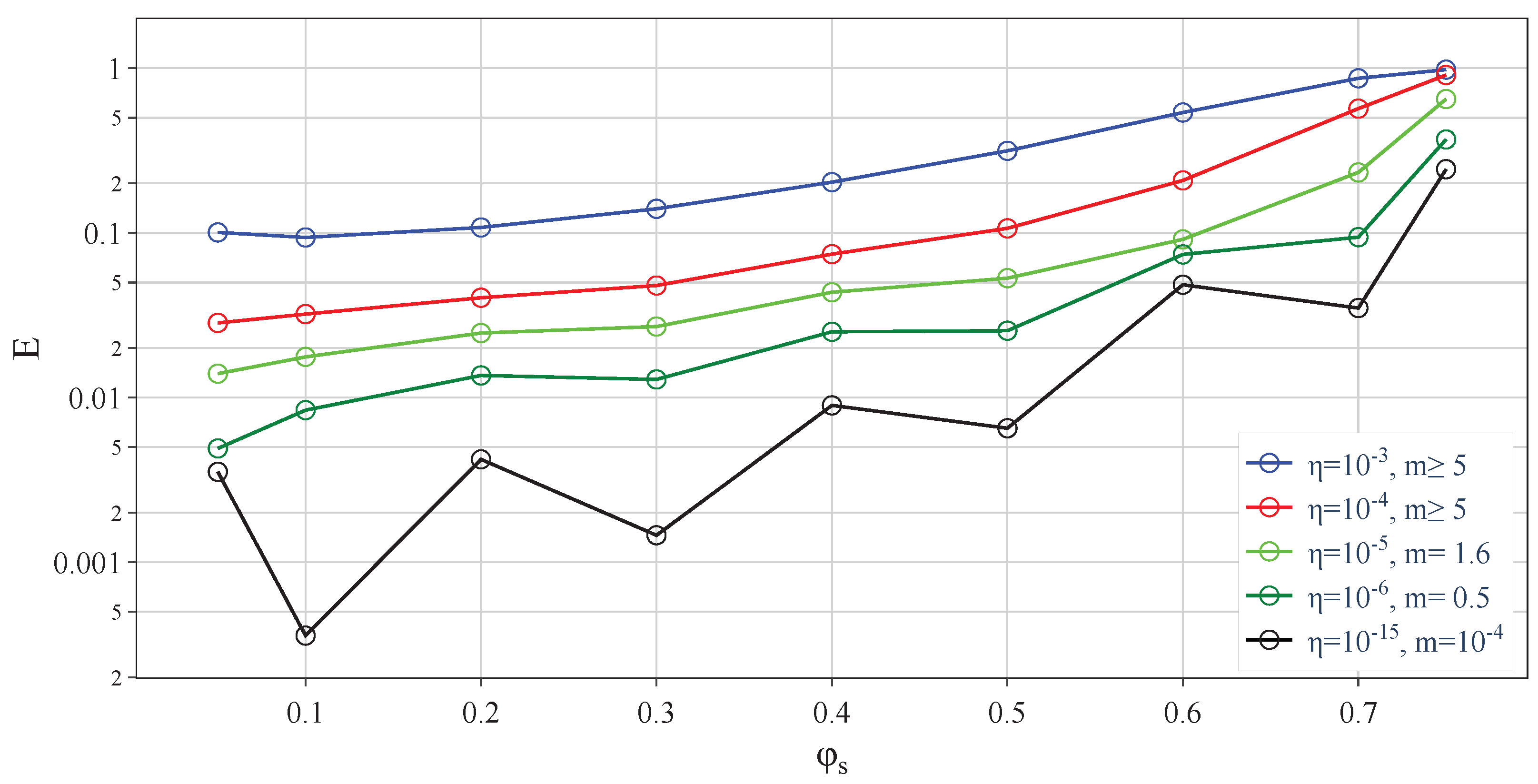
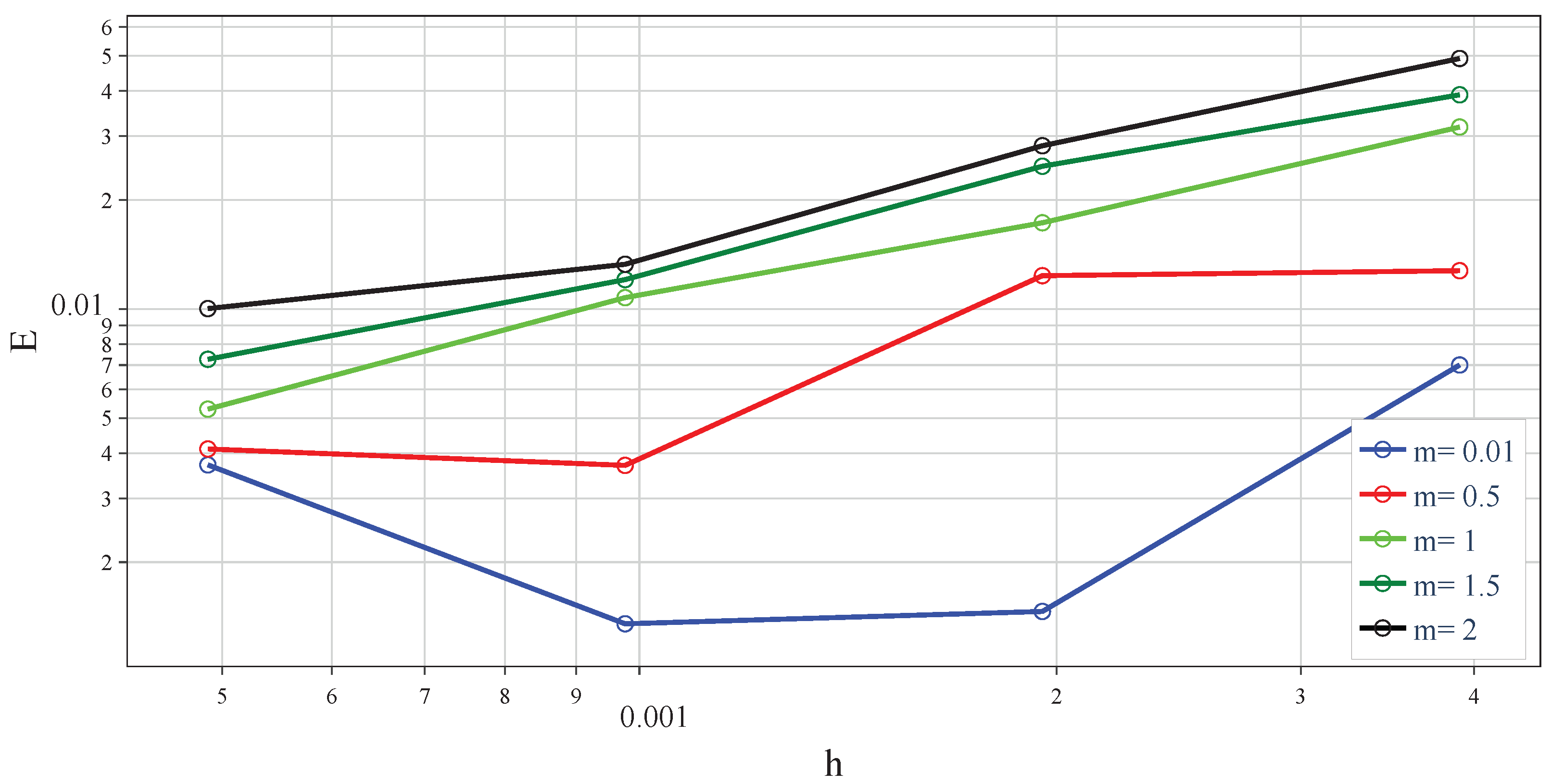
To demonstrate the convergence of
as
decreases, we fixed the maximum level of refinement at
and varied
, as shown in
Figure 4. The convergence depends on the number of cells
per Brinkman layer
(see Equation (
11)). It can be seen that the increase of
m leads to the deterioration of accuracy. As mentioned before, the Brinkman term in the momentum equation models a solid as a porous medium with small permeability, the latter corresponding to small values of
. Thus,
should be taken as small as possible. The decrease of
m, and consequently of
, leads to the decrease of the error. However, at
, when the Brinkman layer is under-resolved, the error oscillates with
, indicating a lack of convergence. The values
or
appear to be optimal in the sense that they are small enough, and yet, the error decreases monotonically. In
Figure 5, we display the grid convergence of the error
E as
for different levels of resolution of the Brinkman layer. The rate of convergence is seen to be about
when
, while at a smaller
m, the monotonicity or even convergence is lost.
To summarize, convergence of the method can be guaranteed provided that: (1) fine features are properly resolved by using sufficiently large levels of refinement ; (2) the number of cells in the Brinkman layer is but not too large; and (3) the penalization coefficient satisfies the estimate .
4.2. Decaying Vortex Problem
The previous test validated the steady-state predictions. To investigate dynamical consistency, we consider the problem of a two-dimensional decaying vortex for which an analytical solution is known. Specifically, the two-dimensional Navier–Stokes equations are solved exactly by the following velocity components:
, and pressure
p [
88] representing a periodic array of vortices decaying exponentially in time:
Here, the fluid density is taken as 1, while the characteristic velocity and length are both taken as 1. The Reynolds number Re is then the reciprocal of the kinematic viscosity .
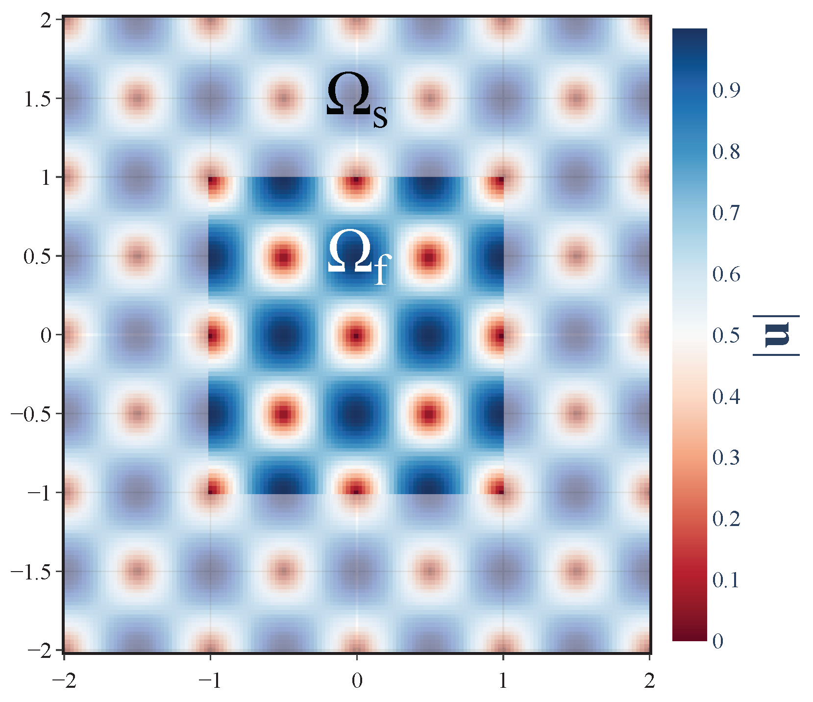
We take as the computational domain a square of size
:
, as shown in
Figure 6. We split the domain into two parts: an inner square
of size 2 and a frame
around the inner square, which is used as a penalization region [
89,
90]. Therefore, the mask value
inside
is 0, while in
, it is 1. The velocity inside the frame
is fixed and given by Equation (
28), while the velocity in
is predicted numerically, starting with the analytical solution in Equation (
28) at
, and its consistency with the exact solution in Equation (
28) at time
is verified. Some other parameters used in the simulation are: the CFL number
, and the tolerance for the Poisson solver is
.
We point out here an aspect of the present computation that is important in general. One must pay careful attention to the selection of fields according to which the grid is adapted giving a higher priority to the fields that reflect the main physical features of the flow. In the case at hand, adaptation on both the velocity and the frame mask was used during the first time step of the computations. Subsequently, the adaptation was performed only on the velocity field . This decision was based on the following observations: (1) the velocity field captures the main physical characteristics of the flow; (2) adaptation on sharp masks leads to the maximum refinement for any adaptation threshold on interfaces even for smooth physical fields () and, therefore, results in excessive use of computational resources without necessarily improving the accuracy of computations.
Ideally, during simulations, the maximum level of refinement
should not be reached; otherwise, this would indicate the general lack of resolution and the need for more refinement. The current level of refinement in all cells should be less than
. The adaptation algorithm should automatically adjust the mesh in the required regions for a specified threshold
. In practice, however, adaptation is often done on masks or other interfaces (
, etc.), which typically have sharp boundaries that require maximum adaptation, and thus, the maximum level of refinement is always reached [
79]. Then, unless specifically tracked, one may miss flow regions away from the masks in which
is also reached and where there is therefore a lack of resolution. One must be careful to avoid such situations.
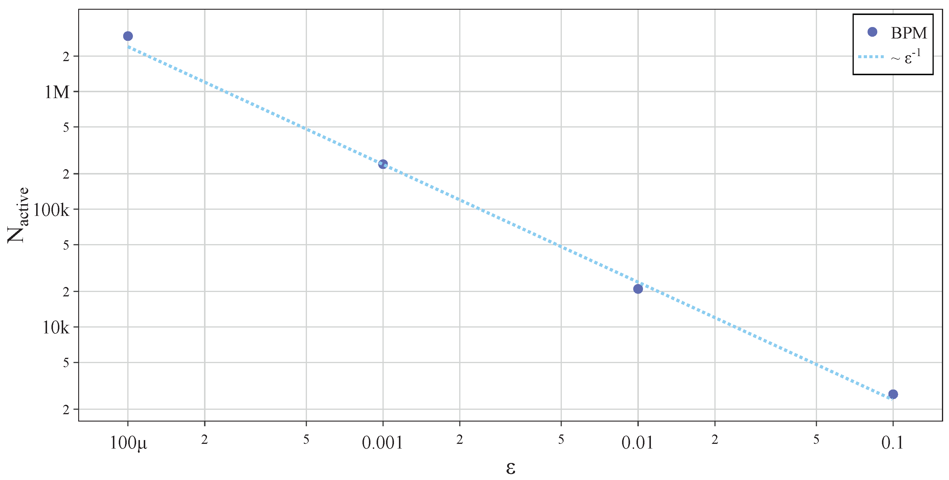
In what follows, we choose the maximum level of refinement as
. We observe that this number is never reached in practice, so
. Recall, our adaptation is done based on
, except for the first time step, when it is done additionally on the mask
. The grid size
h remains in the range from
to
. To monitor the resolution, we plot the dependence of the number of active cells on
in
Figure 7. The number of active cells is seen to be inversely proportional to the adaptation threshold,
. According to ([
91], Equation 3.9), the number of active cells is related to the order of the numerical scheme as
where
s is the discretization order,
n is the dimensionality of the problem (
in the present case), and
is a constant depending on the problem but not on the numerical scheme. From this relation, we derive that the discretization order is
, which is consistent with the order of the numerical scheme.
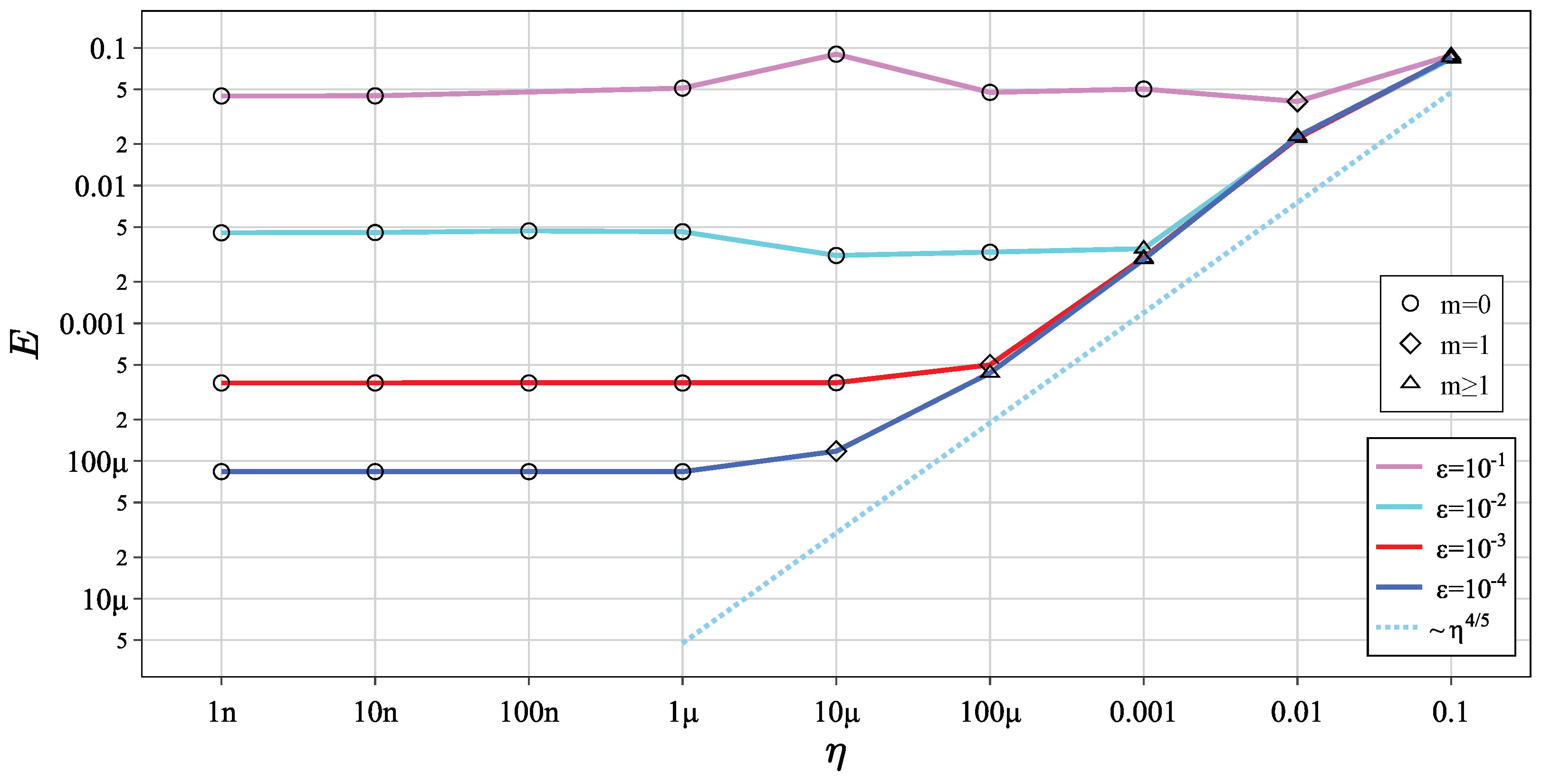
The convergence with respect to the penalization coefficient
and adaptation threshold
is shown in
Figure 8. It is observed that the numerical error decreases with
approximately as
. Note that this order is between
and
seen in Equation (
10). The convergence rate lies between these functions because both normal and tangential components of the speed exist on the interface of the penalty area
. The error is seen to reach a plateau as
becomes very small, and the Brinkman layer is no longer resolved. A similar observation of plateau is found in [
92], where the BPM is used to simulate compressible flows. The reason behind this phenomenon is that the Brinkman layer is not resolved properly and that
along the plateau. Convergence is also seen with the decrease of
.
4.3. Mass Conservation
In BPM, the solid phase is modeled as a porous medium with the porosity controlled by the penalization coefficient
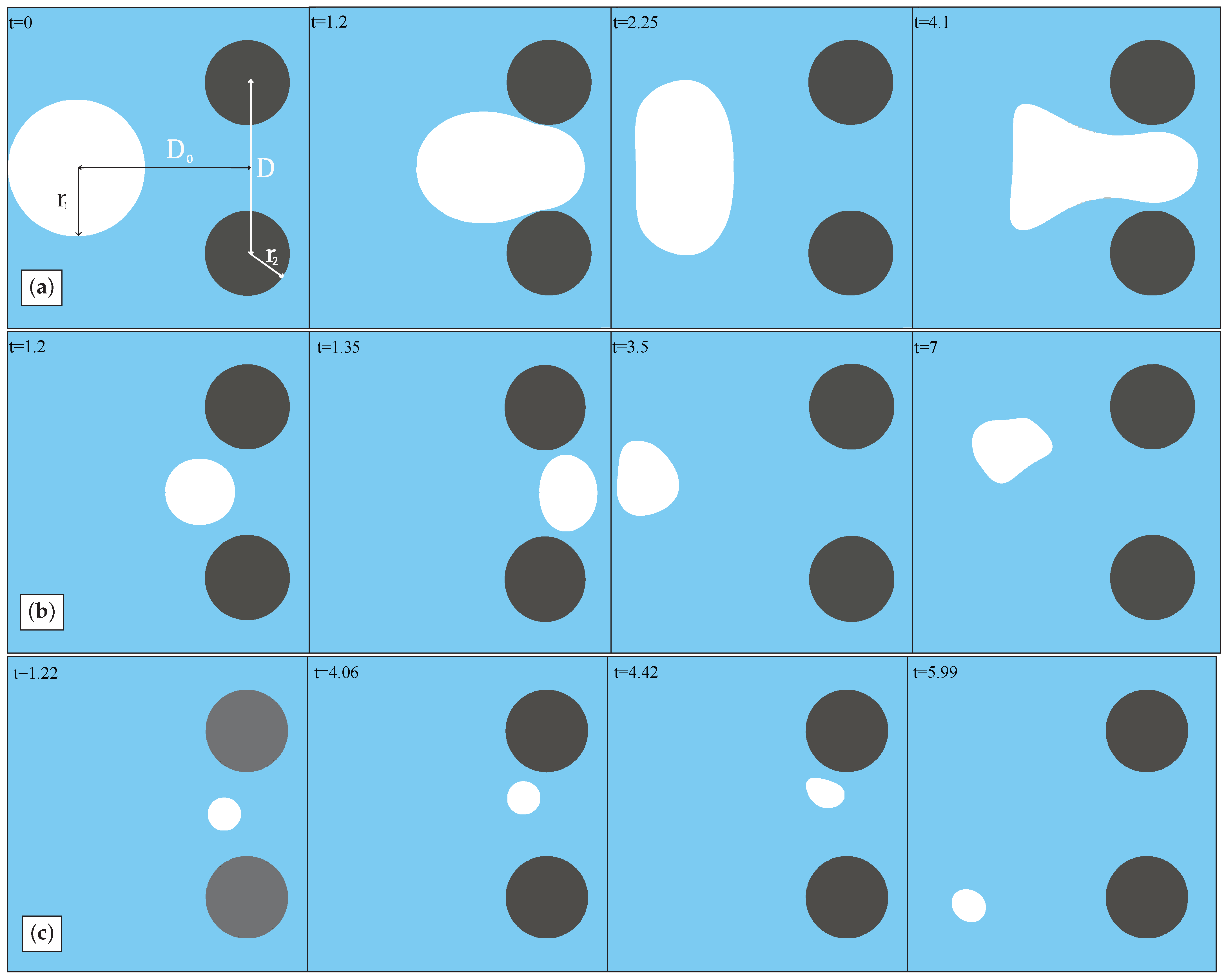
. Therefore, the fluid phase can penetrate the porous solid leading to an apparent mass loss of the fluid. Of course, one should minimize this mass loss as much as possible. In order to evaluate the severity of the problem and to verify the conservation properties of the present method, we consider the following test problem. A bubble of radius
is placed initially next to two identical fixed solid cylinders of radius
, as shown in
Figure 9. The fluids are assumed to be at rest initially. The flow is initiated by gravity
directed from left to right. Because of the left–right periodic boundary conditions, the bubble passes between the obstacles multiple times (more than 15). The bubble undergoes severe deformations in the process, especially in the case of the large bubbles, as shown in
Figure 9. The purpose of this test is to verify conservation of the mass of the bubble after many such cycles.
Important dimensionless parameters that control the dynamics of the bubble in this problem are the capillary number
, the Reynolds number
, and the Froude number
, with
U denoting the mean velocity of the flow,
L the domain size,
the surface tension coefficient, and
,
the density and viscosity of the carrier fluid, respectively. We nondimensionalize the variables as follows:
where the domain size is
mm, and the velocity is
. Then the rescaled domain is a square with a unit side. The mesh adaptation occurs based on the volume fractions
,
, and velocity components
with the corresponding adaptation thresholds
,
, and
. Other parameters are given in
Table 2. The system corresponds to an air bubble in water as a carrier fluid.
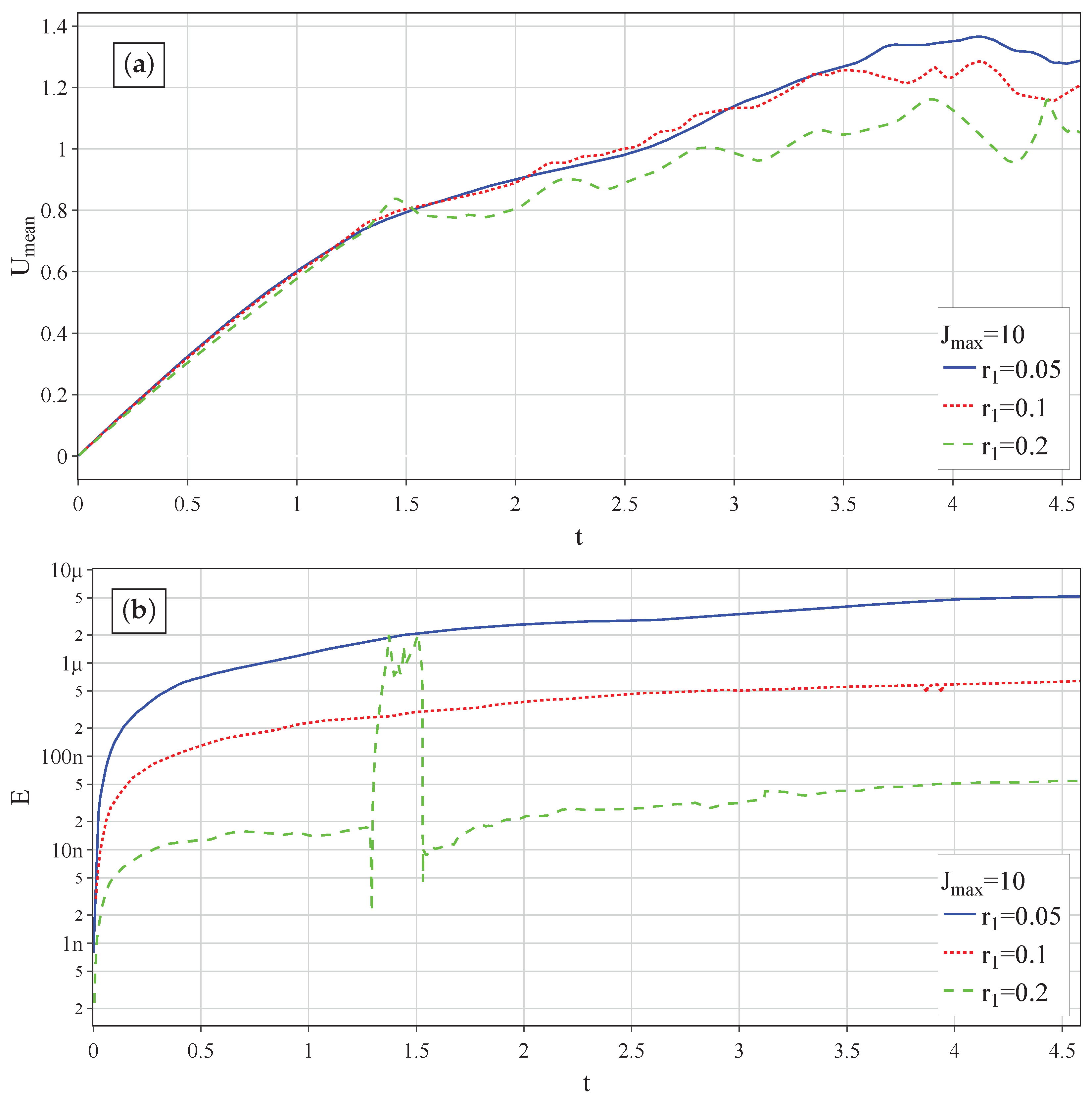
Figure 10a displays the mean velocity of the flow,
, as a function of time for the bubbles of different size. The steady-state mean velocity is seen to be smaller for the larger bubbles as expected due to their stronger interaction with the cylinders.
Figure 10b displays the values of the relative error
of the bubble mass as a function of time. As mentioned above, some error in the mass conservation is expected due to the Brinkman penalization term. In addition, the approximation errors of the overall algorithm, such as of the Poisson solver, will also contribute. However, we note that the error in the mass conservation is consistently at a value of the tolerance of the Poisson solver and does not increase appreciably with time during the simulation. If the bubble radius is smaller than the gap, we observe an initial monotonic increase of the error, which eventually saturates after multiple passages through the gap. In contrast, for the larger bubbles, we notice a sudden jump in the error during the first passage between the cylinders at around time
,
Figure 10b. The large error is evidently due to the stronger interaction between the bubble and the obstacles. Importantly, these larger errors decrease back to the pre-interaction levels once the bubble squeezes between the obstacles. This indicates that even though some fluid mass may be entering the solid during the strong interaction, it is eventually recovered.
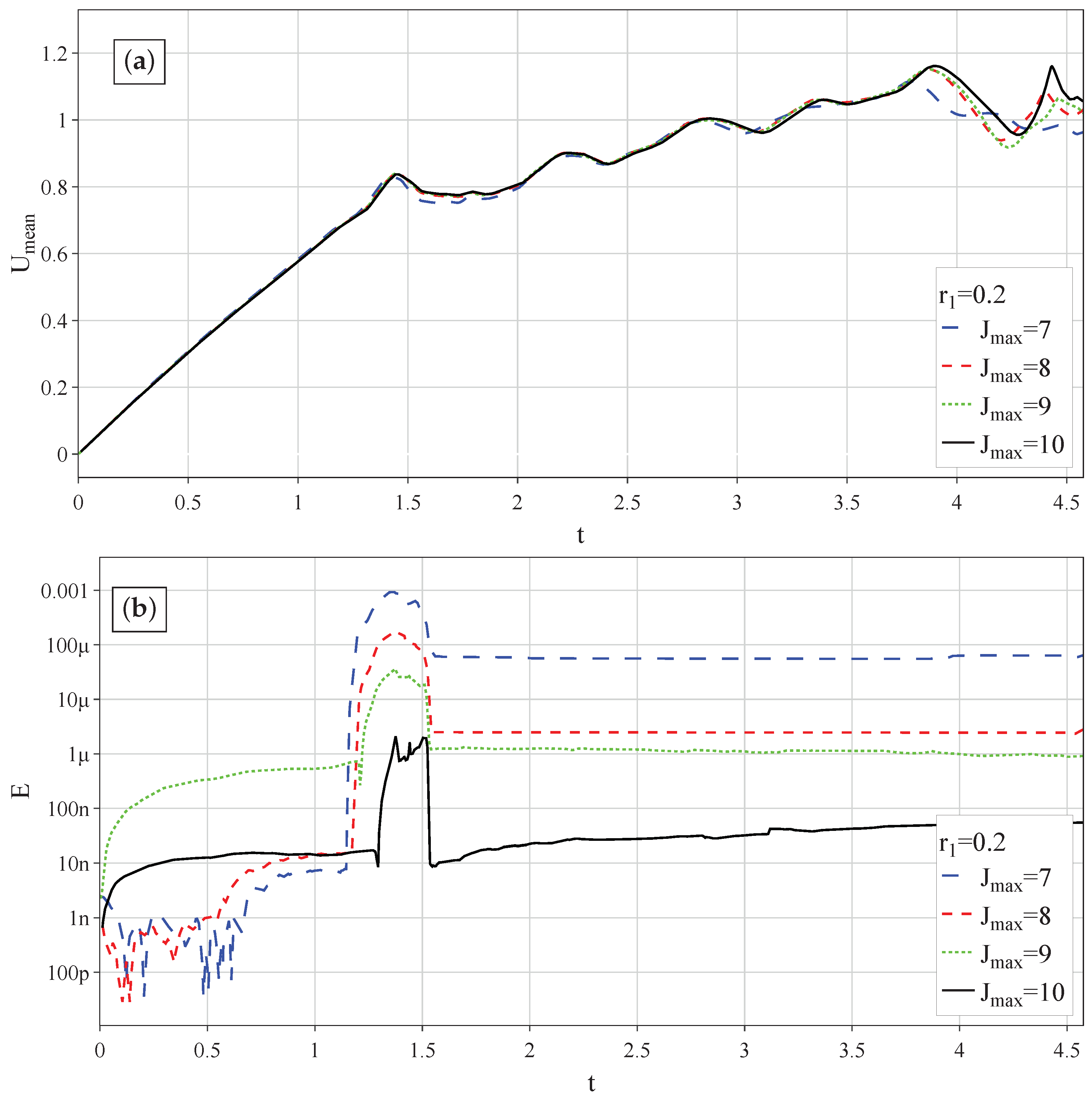
In
Figure 11, we show the mean velocity and the mass conservation error as functions of time for the hardest case of a large bubble with a radius of
when the level of refinement is varied. The important observation is that there is convergence as
increases. The level of error is generally small, and
is at the level of Poisson solver’s tolerance.
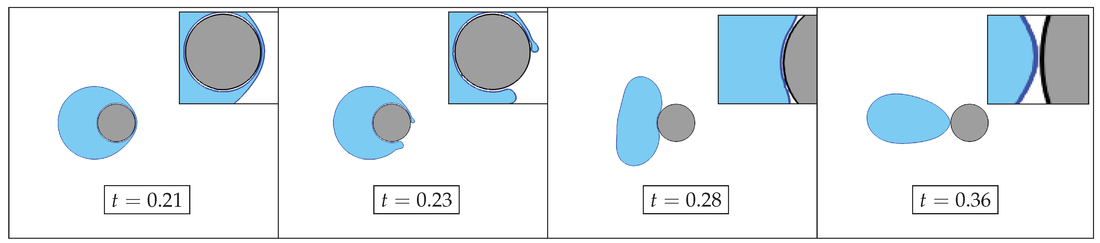
4.4. Multiphase Flows around Moving Solids
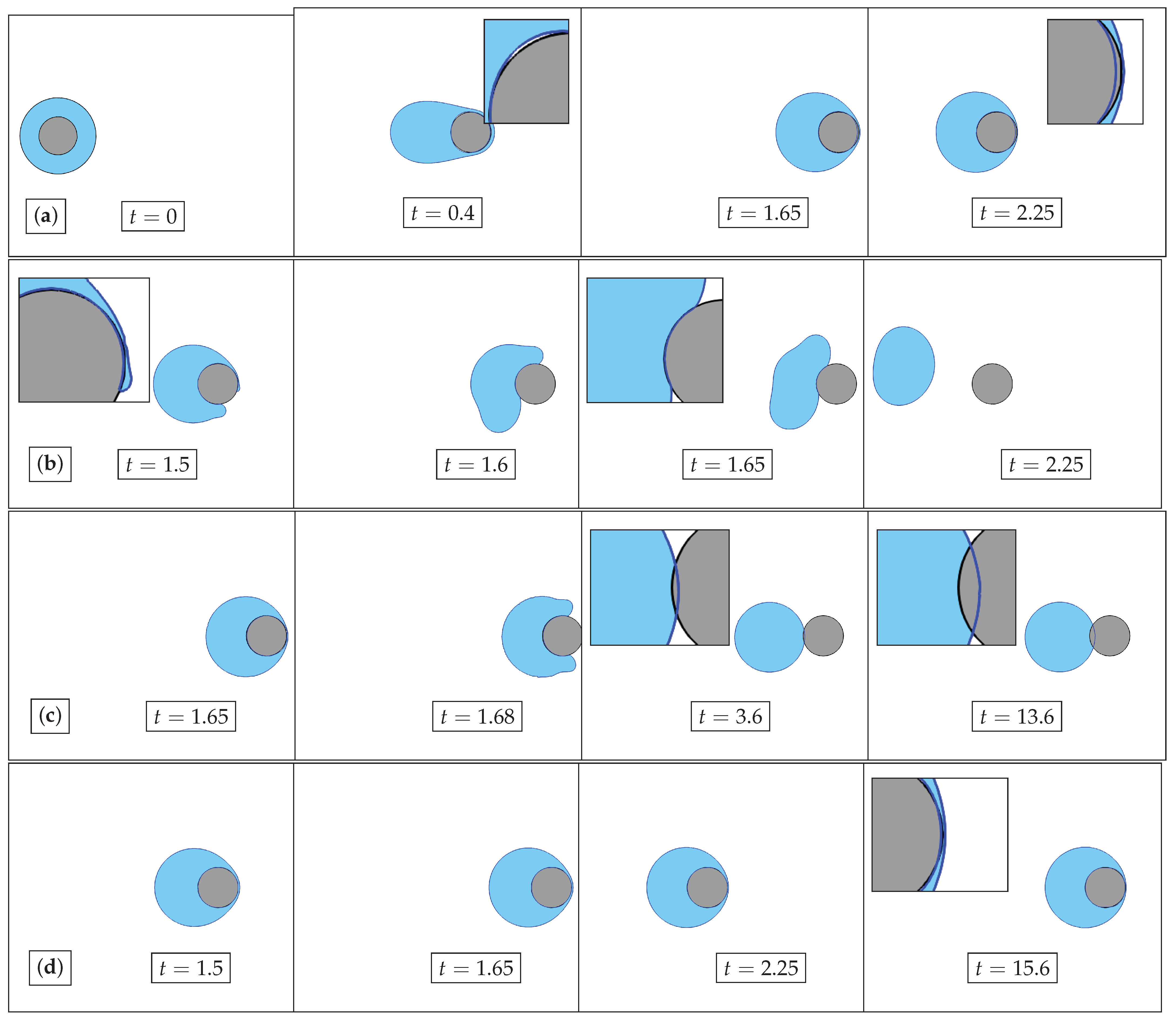
In this section, we consider a two-phase system consisting of a composite droplet moving in a carrier fluid. The computational domain is a square with side
with periodic boundary conditions on the left and right and symmetry boundary conditions on the bottom and top. The composite droplet consists of a solid particle of radius
embedded inside a fluid shell with the outer radius
, as shown in
Figure 12a. The hydrophobic surface of the solid is modeled by
inside the solid, see Equation (
7). Initially, the fluid and the droplet have zero velocity, but the solid particle has a prescribed constant velocity
in the
x direction. The Reynolds and capillary numbers are taken as
and
. The densities and viscosities of both fluids are chosen to be the same and equal to
and
, respectively. The surface tension is equal to
. As the particle moves, it causes the fluids to move as well, and our goal is to simulate the resultant motion.
The numerical simulations are carried out using various treatments of the interaction between the fluids and the solid. We use
as the level of resolution.
Figure 12 displays the results. As the solid moves to the right, the fluid shell moves with it but lags behind due to inertia and the drag with the surrounding fluid. The shell turns into a thin film on the front side of the solid, which can subsequently rupture, and the resultant drop surrounding the solid can detach from it. The simulations using different treatments of the interaction between the solid and the fluid yield different scenarios for the process, and these are explained below.
The method proposed in this work is compared with the simple splitting method (SSM, see
Section 4.1). Recall that in SSM, the cell-centered velocity update is given by
, where
is the velocity field calculated without accounting for the presence of solids.
Figure 12a shows the results based on the application of SSM without this correction. A close look at the solid surface shows that the shell fluid gradually penetrates into the interior of the solid. A similar artifact is seen on the back side of the solid as well, but this time fluid 2 gets out of the solid region at time
(recall that inside the solid,
indicates the presence of the fictitious fluid 2).
The penetration problems can be generally handled by various correctors of the
face velocity
. For example, the usage of the linear corrector
in SSM gives topologically different results, as shown in
Figure 12b, where at some point the particle ruptures the fluid shell. No significant penetration into the solid is seen for the duration of the interaction. It should be noted that the application of SSM for this problem results in poor convergence of the Poisson solver, and subsequently, at large times, the overall error can be substantial (see the
Supplementary Materials Movie S1).
In
Figure 12c, we show the results based on BPM without the correction of
. It is seen that the shell breaks symmetrically (see
) in contrast to
Figure 12b. Additionally, the film ruptures at a later time compared to the SSM with the corrector from Equation(
29). Importantly, now the drop that forms behind the solid does not detach due to the fluid penetration effect. The penetration region continues to increase with time (compare the results at time
and
).
The simulation results based on BPM with the nonlinear (due to the indicator function
) corrector in Equation (
15) are shown in
Figure 12d. No appreciable penetration effect is observed until the simulated time
at least (see also the
Supplementary Materials Movie S2). The mass-conservation error is also generally small. It depends primarily on the accuracy of the Poisson solver and the level of refinement
. To quantify the mass conservation properties, we introduce the relative volume error
, where
are fluid volumes at
and
, respectively. This value for BPM is
for
compared to
for SSM or
for SSM with the face-velocity correction for the simulation time
.
There is also a qualitatively different feature in
Figure 12d that must be mentioned. The BPM with the nonlinear correction preserves the fluid shell intact. There is no rupture of the thin film on the front side, and eventually, there is a steady-state translation of the solid with the deformed fluid layer on it. We point out in this regard that in order to accurately and physically model the rupture of the thin film correctly, the underlying mathematical formulation has to incorporate the physics of the contact angle as well as the effects of disjoining pressure when the film thickness becomes too small. Since they are not part of our model, it is natural that the simulation algorithm does not lead to the film break-up. The problems of the contact line motion and of thin-film break-up have of course received much attention in the past (e.g., [
93,
94]). Their incorporation in the present algorithm is the subject of future work.
The final simulation of this problem of a composite droplet considers a situation in which the solid is covered with a very thin layer of fluid 2 that separates the solid from the thicker shell of fluid 1, forming a kind of a lubrication layer with a thickness of
(see
Figure 13). Note that the lubrication layer here and in other simulations below contains 1 or 2 grid points (i.e.,
, with
) so that they are not required to be fully resolved. This simulation is done with the same method as in
Figure 12d, which is BPM with a nonlinear corrector, and is aimed at eliminating the effects associated with the apparent contact angles. We observe that this case differs from the previous one in that the shell fluid now easily detaches from the lubricated solid similar to the case in
Figure 12b. Unlike the latter, however, the rupture remains more symmetric, even though the symmetry is lost with time (see also the video of the process in the
Supplementary Materials (Movie S3)).
We make one additional remark concerning the BPM with the linear corrector in Equation (
29) for which we do not show any simulation results. Such a method gives the result without rupture; however, the fluid penetration into the solid over more than one computational cell is observed at sufficiently large times
.
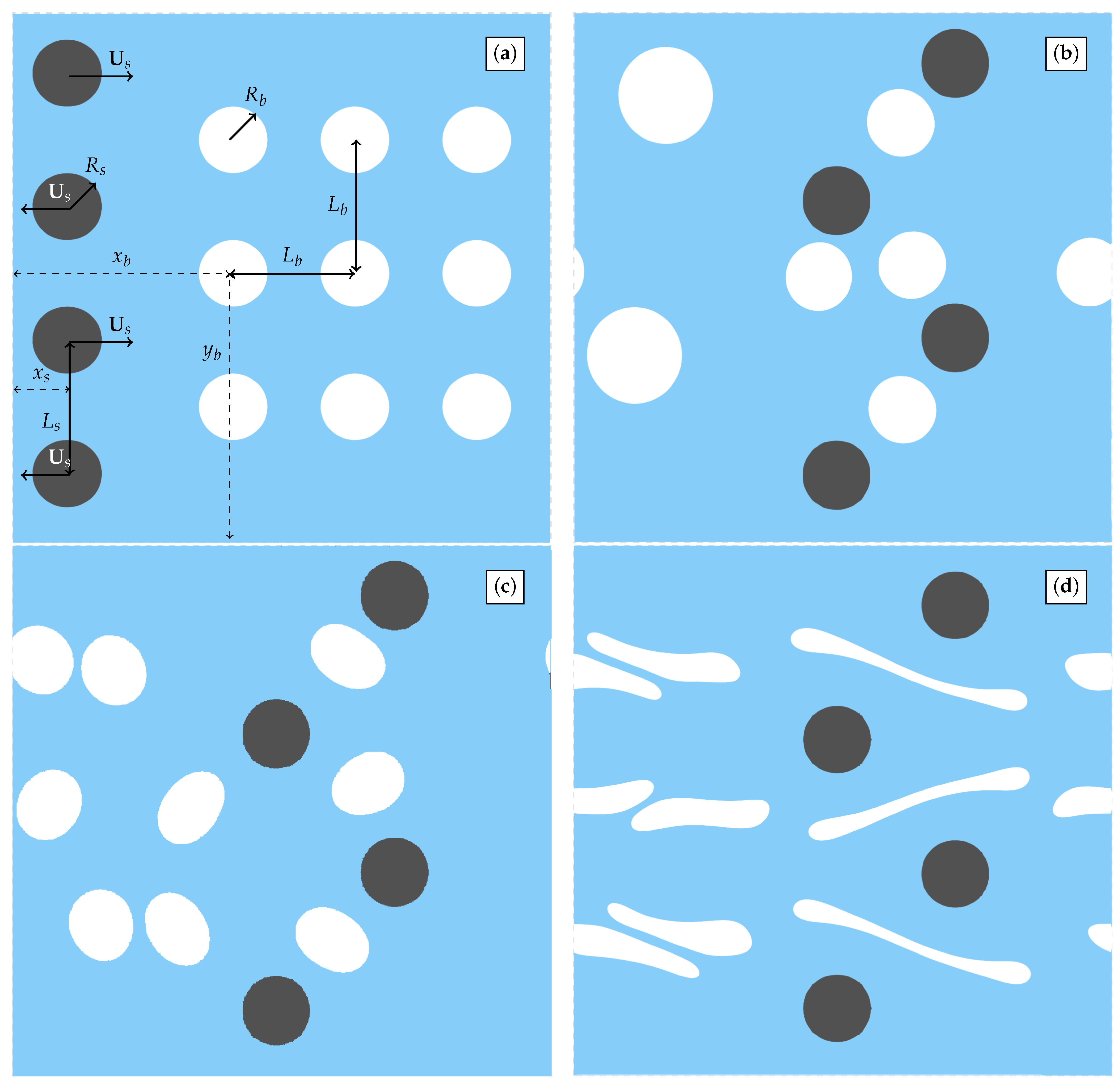
In order to further demonstrate the capabilities of the proposed BPM, we simulate a 2D mixer wherein many solids move in a medium consisting of two fluid phases—the carrier fluid with drops of another fluid moving in it. In
Figure 14a, the schematics of the initial state are shown. The domain size is
, and again, periodic boundary conditions are used. The initial radii of the drops and solid particles are
. Initially, the centers of the four solids are placed uniformly along the
y-axis at
. One of a series of nine drops is arranged at a distance of
and
, as shown in the same figure. The drops are placed in a rectangular order at a distance
in both vertical and horizontal directions. Velocities of the solid particles are directed along the
x-axis in alternating orders with speed
. For simplicity, we assume both fluids have unit density and the same viscosity equal to
. The surface tension is
. Three different capillary numbers
and 1 are used in the simulations to account for the surface tension contribution ranging from dominant to negligible. The solids are assumed to be perfectly wetting.
The results are presented in
Figure 14b–d at time
after two passes of the top solid across the boundary. In
Figure 14b, the simulation is run for
, and some bubbles are found to merge. Increasing Ca, which is the same as decreasing the surface tension, leads to the formation of elongated bubbles with no coalescence (
Figure 14d). A possible qualitative explanation of the latter may be that at large Ca, when the surface tension is small, the bubbles are essentially “enslaved” by the bulk liquid flow and simply follow along that flow. The interaction between bubbles is weak, and hence, coalescence or break-up do not occur easily. In contrast, at large surface tension, the bubbles are more “rigid”, and they transfer the forces from different parts of the surrounding liquid, which leads to their stronger interaction with each other, which, in turn, facilitates coalescence or break-up.
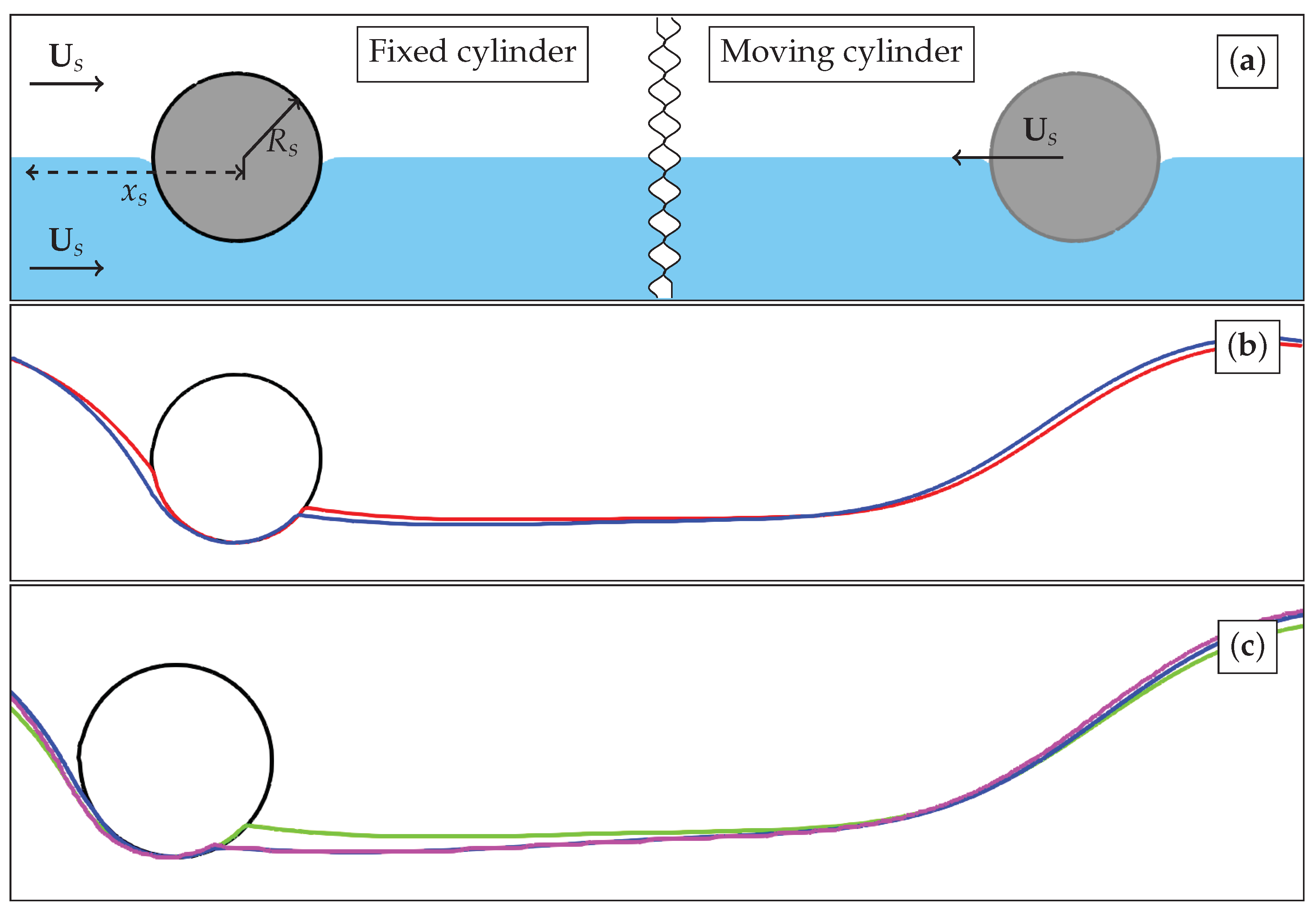
4.5. On Galilean Invariance
In this section, we verify that the proposed algorithm respects the Galilean invariance. For this purpose, we consider the motion of a cylinder or a sphere along an interface between two adjacent fluid layers. We first consider the two-dimensional case in detail and then show an example in three dimensions.
The computational domain is a square , and periodic boundary conditions on the right/left sides and symmetry conditions for top/bottom boundaries are used. We carry out the simulations with two different initial conditions: a fixed cylinder with moving fluids and a moving cylinder with fluids at rest. The radius of the cylinder is . In both cases, the initial difference in speeds is , and the velocity is directed along x. In the case of a moving cylinder, it begins its motion to the left from . In the stationary case, the cylinder is fixed at .
The surface of the solid is assumed to be hydrophobic to the fluid below. Then inside the solid, the fictitious volume fraction field is
. To avoid a sharp corner at the initial position of the contact point where the two fluids and the solid meet, we perform a smoothing operation that deforms the shape of the interface locally near the singular region to make it smoothly touch the solid surface. The smoothing is done using the so-called bounded blending operation, which can generate smooth transitions between two or more surfaces [
95]. The result of smoothing is shown in
Figure 15a.
In
Figure 15b, the numerical results for the moving and fixed cases are compared at time
when the solid positions coincide. This figure shows that the solid surface appears to be partially wet (for example, the apparent contact angle on the back side (i.e., to the right) is about
). At the same time, the front side of the moving solid remains non-wetting. Clearly, this behavior misrepresents the real physics of the fluid–solid contact. Such serious discrepancies in the interface position near the solid contact region (and therefore everywhere else) arise due to the various features of the numerical algorithm, such as the flux corrections and the time splitting. As an additional (and likely related) difficulty, we observe no convergence of the contact-point positions with mesh refinement for the levels of refinement
, or 11 (see
Figure 15c).
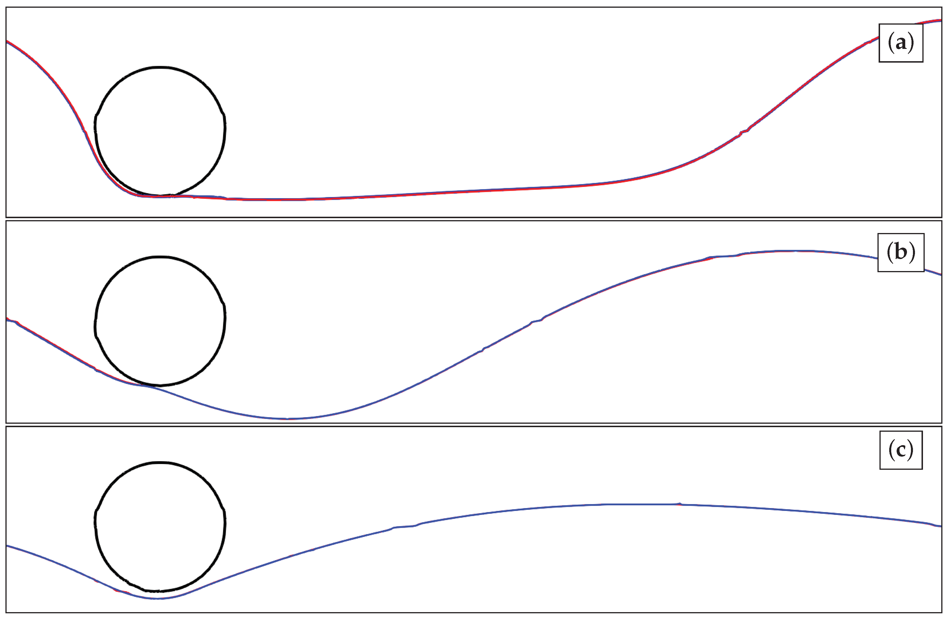
In order to remedy the problem of the apparent contact angles in
Figure 15b, we resort to the same approach as was taken in producing
Figure 13. That is, we model the hydrophobic surfaces with a thin lubrication layer around the solid. The film thickness is taken as
. The results are shown in
Figure 16 at three times corresponding to the first three coincidences of the moving and fixed solids (recall, the motion is left–right periodic with the domain length 1, and the cylinder velocity is also 1). In all three time frames, the new algorithm is seen to respect the Galilean invariance with excellent accuracy. See also the
Supplementary Movie S4.
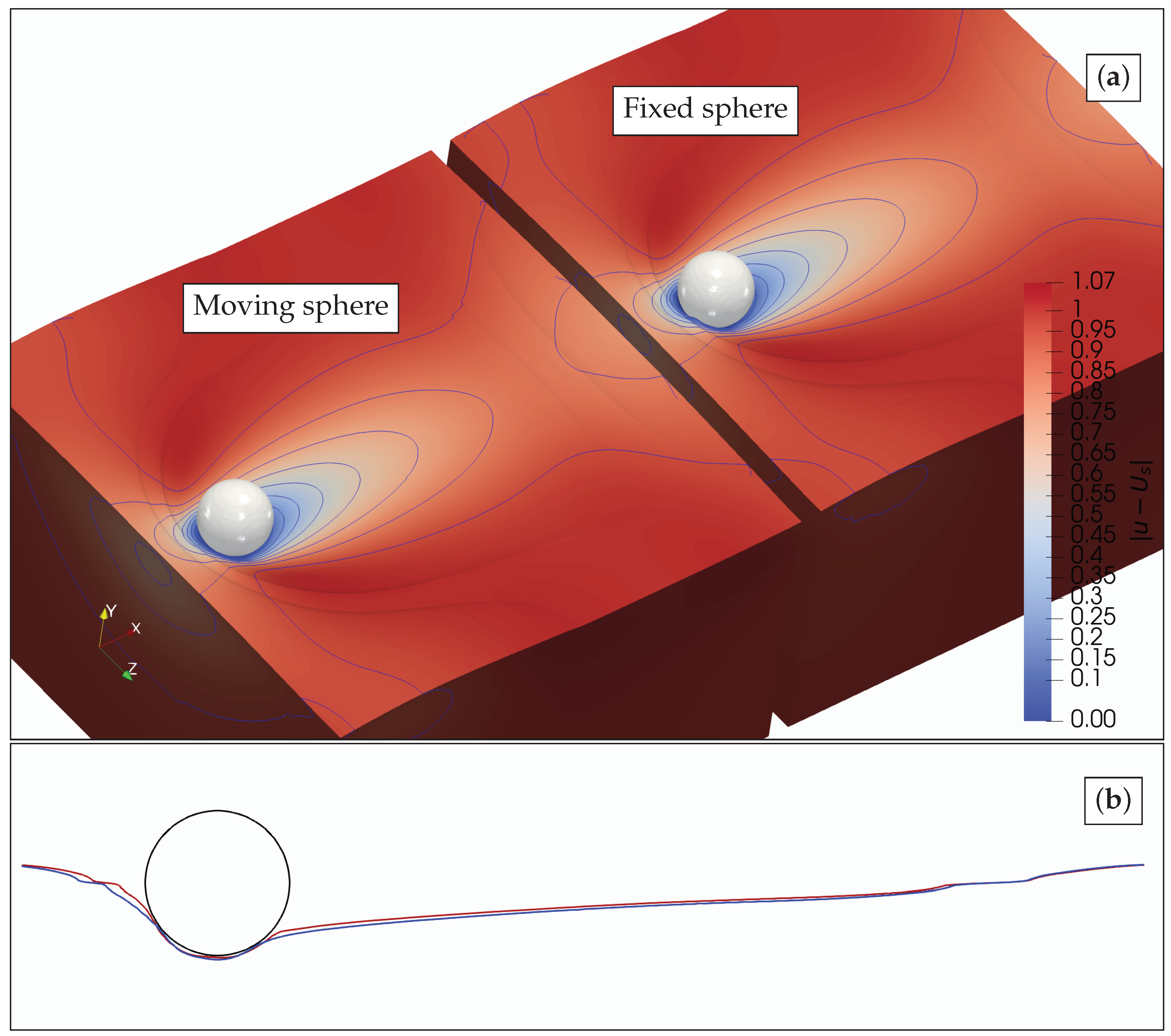
All of the simulations above considered two-dimensional problems for simplicity. The algorithm is, however, developed for general three-dimensional problems. Next, we demonstrate the application of the method to the problem of a sphere moving along the interface between two fluids, which is an extension of the previous result to three dimensions. The simulation was carried out in a domain
, and the results are shown in
Figure 17. The figure displays the solid and fluid interfaces at time
. Additionally, the color levels and isocontours on the interface indicate the norm of the relative velocity
. We can see that the form of the isolines is practically the same for both the moving and stationary sphere, which confirms the Galilean invariance in this case as well. The video of the three-dimensional simulation is in the
Supplementary Movie S5.
5. Conclusions
In this work, we have contributed to the development of an algorithm for the simulation of multiphase flows consisting of several incompressible fluids and solid objects, the latter either stationary or moving with a prescribed velocity. The solids are assumed to be either perfectly superhydrophilic or perfectly superhydrophobic so that no contact-angle effects are considered. The core of the algorithm consists of the Brinkman penalization method to handle the solids, the volume of fluid method to handle the fluid interfaces, and the continuous surface force to model surface tension phenomena.
The algorithm is implemented in the open source solver Basilisk [
1,
52] and is validated with a number of test cases. Simulations in Basilisk use adaptive Cartesian meshes that are highly efficient in capturing multiscale features of complex flows, such as the multiphase flows considered in this work. In particular, the algorithm is tested on the problems of Stokes flow past a periodic array of cylinders and of a decaying vortex flow for which there exist analytical solutions. The convergence of the method is demonstrated not only with an increasing grid resolution but also with a decreasing penalization coefficient
.
In addition, we have calculated the flow of a carrier fluid with bubbles and with several stationary or moving obstacles. The mass conservation property of the algorithm and its ability to handle the motion of a solid in a two-phase fluid is verified with a problem of a bubble squeezing between two solid obstacles and a problem of a solid breaking out of a surrounding fluid shell. Another case that we have simulated involves mixing multicomponent fluids by means of moving solids. This problem demonstrates the ability of the algorithm to handle complex deforming interfaces and interactions between different fluids and solid obstacles. Lastly, we have verified that the algorithm satisfies the Galilean invariance. This test is carried out with a solid cylinder or sphere moving along an interface separating two different fluids.
Thus, we have demonstrated that the algorithm can accurately and efficiently handle a wide range of complex multiphase flow problems. Nevertheless, we point out some of the underlying assumptions that must be relaxed in order to extend the range of problems that can be simulated. One of the main assumptions is that the solid phase motion is assumed prescribed. Obviously, in practice, this is often not the case, and the fluid and solid motions are fully coupled. Another assumption is that of the incompressibility of all the fluid phases involved. Even though this is not such a strong limitation in many applications, the treatment of, say, bubbly liquids may require relaxing the incompressibility assumption about the gas.
Important additional physics that can be incorporated into the modeling and in the algorithm is that of the finite contact angle. As presented, the algorithm assumes that the solids are either perfectly superhydrophobic or perfectly superhydrophylic. The numerical treatment of these cases is also not without difficulties, especially when a solid moves in a two-phase medium. Our simulations with a composite droplet (a solid particle within a fluid shell) moving in an external fluid have shown that many numerical artifacts arising with different approaches to the treatment of the interaction between the solid and the fluids can be eliminated with an approach that allows for a thin (1–2 mesh cells) lubrication layer on the solid surface. Implementing this idea allows for the treatment of both stationary and moving solids with a physically correct and accurate representation of the interaction between the solid and fluids. The solution involving the lubrication layer avoids overlapping different sharp transition layers coming from the fluid–fluid and fluid–solid interfaces contributing to the robustness of the method.


