
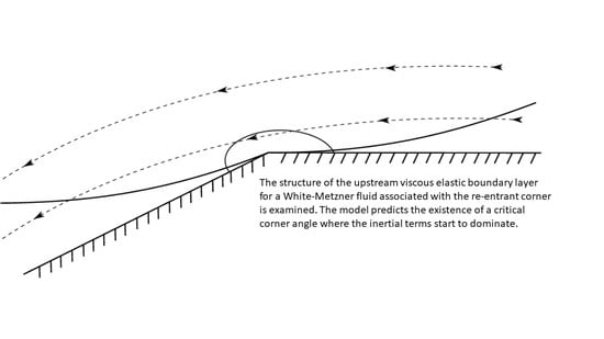
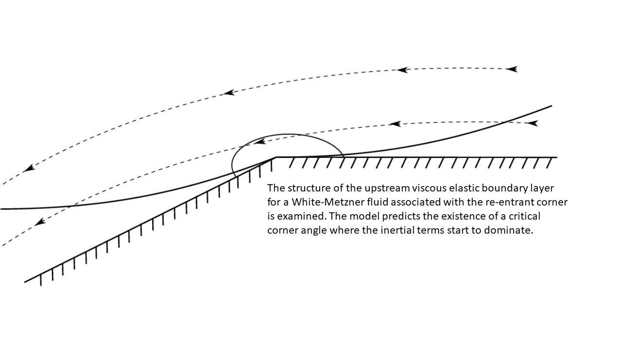
Re-Entrant Corner for a White-Metzner Fluid


Abstract
:
1. Introduction
2. Materials and Methods
Governing Equations
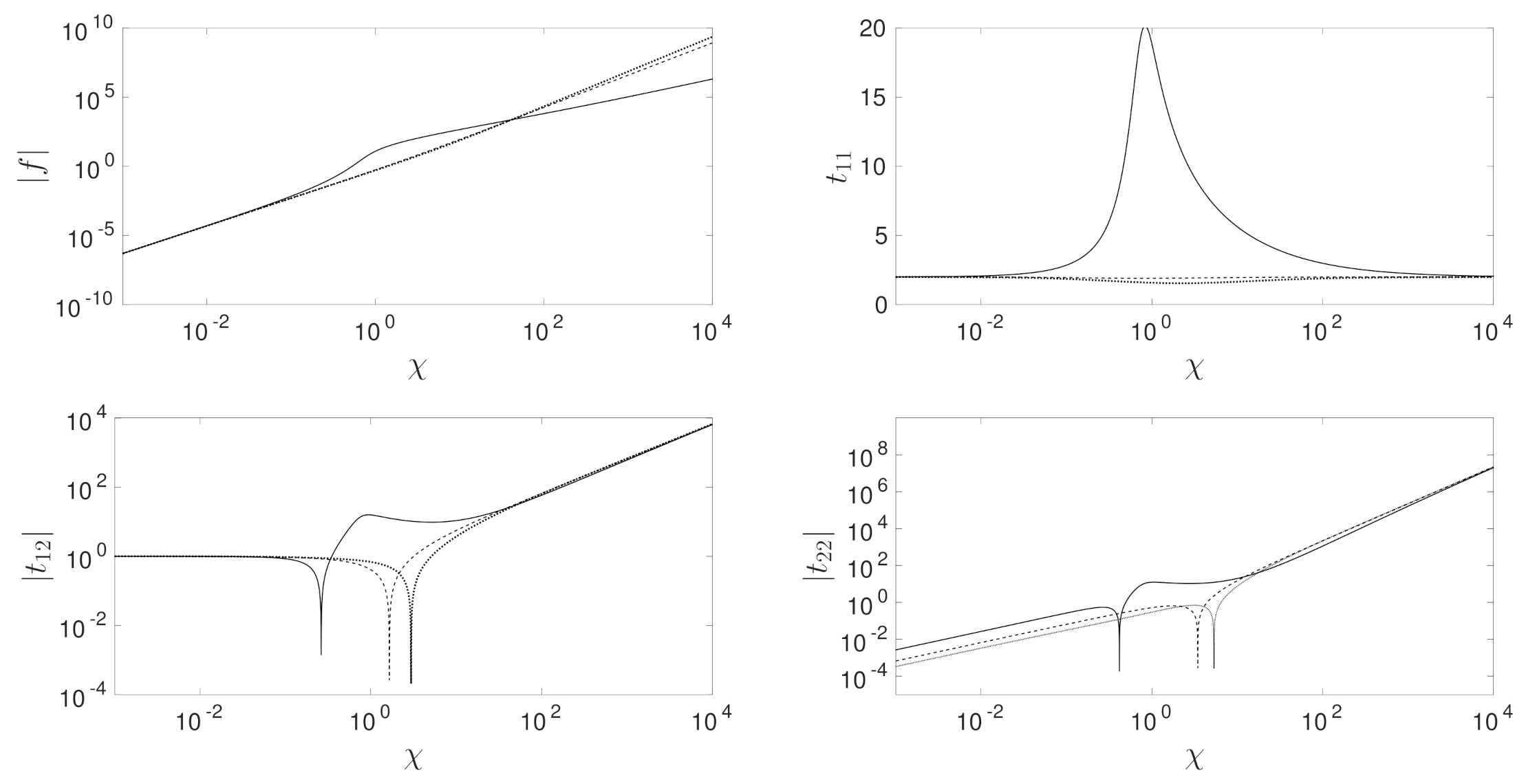
3. Results
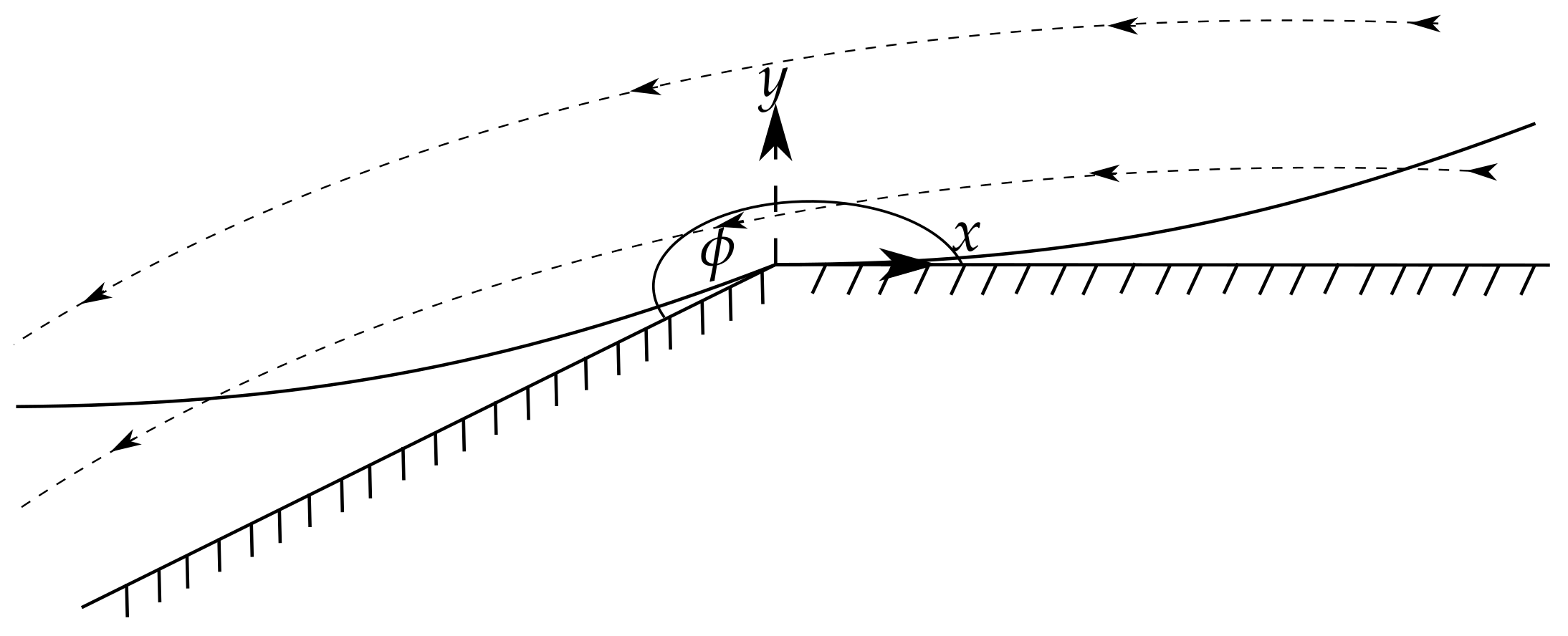
3.1. Boundary Layer Analysis
Outer Solution
- (I)
- ,
- (II)
- ,
- (III)
- ,
- (IV)
- .
3.2. Upstream Boundary Layer
3.3. Similarity Solution
Near Wall Analysis
3.4. Upstream Boundary Layer
4. Discussion
Author Contributions
Funding
Conflicts of Interest
Abbreviations
| PTT | Phan-Thien-Tanner |
| UCM | upper-convective Maxwell |
| WM | White-Metzner |
Appendix A. Series Expansion Terms
Appendix B. Parameters
Appendix C. Constraint
References
- Prandtl, L. Motion of fluids with very little viscosity. In Technical Memorandum, 452; National Advisory Committee for Aeronautics: Washington, DC, USA, 1928; pp. 1–8. [Google Scholar]
- Chaffin, S.T.; Rees, J.M. Carreau fluid in a wall driven corner flow. J. Non-Newton. Fluid Mech. 2018, 253, 16–26. [Google Scholar] [CrossRef]
- Schowalter, W.R. The application of boundary-layer theory to power-law pseudoplastic fluids: Similar solutions. AIChE J. 1960, 6, 24–28. [Google Scholar] [CrossRef]
- Evans, J.D.; Hagen, T. Viscoelastic sink flow in a wedge for the UCM and Oldroyd-B models. J. Non-Newton. Fluid Mech. 2008, 154, 39–46. [Google Scholar] [CrossRef]
- Boger, D.V.; Crochet, M.J.; Keiller, R.A. On viscoelastic flows through abrupt contractions. J. Non-Newton. Fluid Mech. 1992, 44, 267–279. [Google Scholar] [CrossRef]
- Hassell, D.G.; Auhl, D.; McLeish, T.C.B.; Mackley, M.R. The effect of viscoelasticity on stress fields within polyethylene melt flow for a cross-slot and contraction-expansion slit geometry. Rheol. Acta 2008, 47, 821–834. [Google Scholar] [CrossRef]
- Singh, P.; Leal, L.G. Finite element simulation of flow around a corner using the FENE dumbbell model. J. Non-Newton. Fluid Mech. 1995, 58, 279–313. [Google Scholar] [CrossRef]
- Cruz, F.A.; Poole, R.J.; Afonso, A.M.; Pinho, F.T.; Oliviera, P.J.; Alves, M.A. A new viscoelastic benchmark flow: Stationary bifurcation in a cross-slot. J. Non-Newton. Fluid Mech. 2014, 214, 57–68. [Google Scholar] [CrossRef]
- Rocha, G.N.; Poole, R.J.; Alves, M.A.; Oliviera, P.J. On extensibility effects in the cross-slot flow bifurcation. J. Non-Newton. Fluid Mech. 2009, 156, 58–69. [Google Scholar] [CrossRef] [Green Version]
- Lipscomb, G.G.; Keunings, R.; Denn, M.M. Implications of boundary singularities in complex geometries. J. Non-Newton. Fluid Mech. 1987, 24, 85–96. [Google Scholar] [CrossRef]
- Hinch, E.J. The flow of an Oldroyd fluid around a sharp corner. J. Non-Newton. Fluid Mech. 1993, 50, 161–171. [Google Scholar] [CrossRef] [Green Version]
- Renardy, M. The stresses of an upper convected Maxwell fluid in a Newtonian velocity field near a re-entrant corner. J. Non-Newton. Fluid Mech. 1993, 50, 127–134. [Google Scholar] [CrossRef]
- Renardy, M. A matched solution for corner flow of the upper convected Maxwell fluid. J. Non-Newton. Fluid Mech. 1995, 58, 83–89. [Google Scholar] [CrossRef]
- Evans, J.D. Re-entrant corner flows of UCM fluids: The Cartesian stress basis. J. Non-Newton. Fluid Mech. 2008, 150, 116–138. [Google Scholar] [CrossRef]
- Rallinson, J.M.; Hinch, E.J. The flow of an Oldroyd fluid past a reentrant corner: The downstream boundary layer. J. Non-Newton. Fluid Mech. 2004, 116, 141–162. [Google Scholar] [CrossRef]
- Renardy, M. The high Weissenberg number limit of the UCM model and the Euler equations. J. Non-Newton. Fluid Mech. 1997, 69, 293–301. [Google Scholar] [CrossRef]
- Evans, J.D. Re-entrant corner flows of Oldroyd-B fluids. Proc. R. Soc. A 2005, 461, 2573–2603. [Google Scholar] [CrossRef]
- Evans, J.D. High Weissenberg number boundary layer structures for UCM fluids. Appl. Math. Comput. 2020, 387, 124952. [Google Scholar] [CrossRef]
- James, D.F. Boger fluids. Annu. Rev. Fluid Mech. 2009, 41, 129–142. [Google Scholar] [CrossRef]
- Evans, J.D. Re-entrant corner flows of PTT fluids in the Cartesian stress basis. J. Non-Newton. Fluid Mech. 2008, 153, 12–24. [Google Scholar] [CrossRef]
- Evans, J.D. Re-entrant corner flow for PTT fluids in the natural stress basis. J. Non-Newton. Fluid Mech. 2009, 157, 79–91. [Google Scholar] [CrossRef]
- Sibley, D.N. Viscoelastic Flows of PTT Fluid. Ph.D. Thesis, University of Bath, Bath, UK, 2010. [Google Scholar]
- White, J.L.; Metzner, A.B. Development of constitutive equations for polymeric melts and solutions. J. Appl. Polym. Sci. 1963, 7, 1867–1889. [Google Scholar] [CrossRef]
- Metzner, A.B.; Whitlock, M. Flow behavior of concentrated (dilatant) suspensions. Trans. Soc. Rheol. 1958, 2, 239–254. [Google Scholar] [CrossRef]
- Boersma, W.H.; Laven, J.; Stein, H.N. Viscoelastic properties of concentrated shear-thickening dispersions. J. Colloid Interface Sci. 1992, 149, 10–22. [Google Scholar] [CrossRef] [Green Version]
- Strivens, T.A. The shear thickening effect in concentrated dispersion systems. J. Colloid Interface Sci. 1976, 57, 476–487. [Google Scholar] [CrossRef]
- Dhanasekharan, M.; Huang, H.; Kokini, J.L. Comparison of observed rheological properties of hard wheat flour dough with predictions of the Giesekus-Leonov, White-Metzner and Phan-Thien Tanner Models. J. Texture Stud. 1999, 30, 603–623. [Google Scholar] [CrossRef]
- Maders, H.; Vergnes, B.; Demay, Y.; Agassant, J.F. Steady flow of a White-Metzner fluid in a 2-D abrupt contraction-computation and experiments. J. Non-Newton. Fluid Mech. 1992, 45, 63–80. [Google Scholar] [CrossRef]
- Raghay, S.; Hakim, A. Numerical simulation of White–Metzner fluid in a 4:1 contraction. Int. J. Numer. Methods Fluids 2001, 35, 559–573. [Google Scholar] [CrossRef]
- Sousa, P.C.; Pinho, F.T.; Oliviera, M.S.N.; Alves, M.A. Purely elastic flow instabilities in microscale cross-slot devices. Soft Matter 2015, 11, 8856–8862. [Google Scholar] [CrossRef] [Green Version]
- Bird, R.B.; Curtiss, C.F.; Armstrong, R.C.; Hassager, O. Dynamics of Polymeric Liquids, Fluid Mechanics; Wiley: New York, NY, USA, 1987; Volume 1. [Google Scholar]
- Liao, T.Y.; Hu, H.H.; Joseph, D.D. White-Metzner models for rod climbing in A1. J. Non-Newton. Fluid Mech. 1994, 51, 111–124. [Google Scholar] [CrossRef]
- Barnes, H.A.; Roberts, G.P. A simple empirical model describing the steady-state shear and extensional viscosities of polymer melts. J. Non-Newton. Fluid Mech. 1992, 44, 113–126. [Google Scholar] [CrossRef]
- Valette, R.; Laure, P.; Demay, Y.; Agassant, J. Investigation of the interfacial instabilities in the coextrusion flow of PE and PS. Int. Polym. Proc. 2003, 18, 171–178. [Google Scholar] [CrossRef]
- Cherizol, R.; Sain, M.; Tjong, J. Review of non-Newtonian mathematical models for rheological characteristics of viscoelastic composites. Green Sustain. Chem. 2015, 5, 6–14. [Google Scholar] [CrossRef] [Green Version]
- Evans, J.D. Re-entrant corner flows of the upper convected Maxwell fluid. Proc. R. Soc. A 2005, 461, 117–141. [Google Scholar] [CrossRef]


| Fluid | n | q |
|---|---|---|
| A | 0.33 | 0.56 |
| B | 0.4 | 0.0 |
| C | 0.29 | 0.11 |
| D | 0.17 | 0.064 |
Publisher’s Note: MDPI stays neutral with regard to jurisdictional claims in published maps and institutional affiliations. |
© 2021 by the authors. Licensee MDPI, Basel, Switzerland. This article is an open access article distributed under the terms and conditions of the Creative Commons Attribution (CC BY) license (https://creativecommons.org/licenses/by/4.0/).
Share and Cite
Chaffin, S.; Monk, N.; Rees, J.; Zimmerman, W. Re-Entrant Corner for a White-Metzner Fluid. Fluids 2021, 6, 241. https://doi.org/10.3390/fluids6070241
Chaffin S, Monk N, Rees J, Zimmerman W. Re-Entrant Corner for a White-Metzner Fluid. Fluids. 2021; 6(7):241. https://doi.org/10.3390/fluids6070241
Chicago/Turabian StyleChaffin, Stephen, Nicholas Monk, Julia Rees, and William Zimmerman. 2021. "Re-Entrant Corner for a White-Metzner Fluid" Fluids 6, no. 7: 241. https://doi.org/10.3390/fluids6070241