1. Introduction
The near-wall grid resolution required to accurately resolve the boundary layer in wall-bounded flows remains a pacing item in large-eddy simulations (LES) for high-Reynolds-number engineering applications. Studies by Chapman [
1], and more recently by Choi and Moin [
2] and Yang and Griffin [
3], estimated that the number of grid points necessary for wall-resolved LES scales is
, where
is the characteristic Reynolds number of the problem. The computational cost is still excessive for many practical problems, especially for external aerodynamics, despite the favorable comparison with the
scaling required for direct numerical simulation (DNS), where all the relevant scales of motion are resolved. Even in LES, the large-scale structures relevant to wall-bounded turbulence, as observed since the early days of flow visualization [
4,
5,
6,
7], need to be adequately resolved in order to obtain accurate predictions using simulations. The alternative to resolving the large-scale structures of the near-wall region is wall modeling. By modeling the near-wall flow such that only the large-scale motions in the outer region of the boundary layer are resolved, the grid-point requirement for wall-modeled LES scales at most linearly with increasing Reynolds number. Therefore, wall-modeling stands as the most feasible approach for wall-resolved LES or DNS.
Examples of the most popular and well-known wall models are the traditional wall-stress models (or approximate boundary conditions) and the detached eddy simulation (DES) and its variants. DES [
8] combines RANS equations close to the wall and LES in the outer layer with the interface between Reynolds-averaged Navier–Stokes and LES domains enforced implicitly through the change in the turbulence model. The traditional wall-stress models impose an approximate boundary condition at the wall rather than a no-slip boundary condition, imposing a wall stress (computed by the model) or the law of the wall through the boundary condition. Deardorff [
9] used a boundary condition based on the law of the wall, imposing a condition on the second derivative of the streamwise velocity in the wall-normal direction. Schumann [
10] used a finite volume approach and a staggered grid and supplied the correct tangential shear stress at the wall as the boundary flux term. Throughout the years, many researchers followed the method of Schumann [
10] for finite difference methods by utilizing a Neumann boundary condition in the wall-parallel velocity components to specify the shear stress at the wall due to the straightforward connection between the wall shear stress and the wall-normal component of the streamwise velocity gradient at the wall [
11,
12,
13,
14]. More recently, Robin boundary conditions in the three velocity components have been employed in wall-modeled large-eddy simulations (WMLES) [
15,
16]. The reader is referred to Cabot and Moin [
12], Piomelli and Balaras [
17], Larsson et al. [
18] and Bose and Park [
19] for a more comprehensive review of wall-stress models.
In most of the instances mentioned above, the eddy viscosity at the wall is assumed to be zero or computed from the subgrid-scale (SGS) model, and is not part of the wall model. Using the eddy viscosity at the wall as a wall-modeling term provides various options in imposing the correct wall shear stress through the stress-balance equation. One such option is to impose a boundary condition on the eddy viscosity at the wall rather than the wall-normal derivative of the streamwise velocity [
20]. In the current study, we compare three different boundary conditions that arise from the mean LES stress-balance equation at the wall wherein a no-penetration (zero wall-normal velocity at the wall) condition is assumed in a finite-difference framework. We will show that augmenting the eddy-viscosity at the wall, rather than imposing a Neumann boundary condition for the wall-parallel velocities, provides a better prediction of the mean velocity profile and turbulence statistics in the first few grid points off the wall.
Better prediction of the mean velocity profile in the first few grid points off the wall has real-world implications for wall modeling. Log-layer mismatch refers to a well-known problem in WMLES where the modeled wall-shear stress deviates from the actual value, either by underpredicting [
14,
21] or overpredicting [
22,
23] the stress. Previous works attempting to solve the issue of log-layer mismatch include works on modifying the SGS stress models [
24], using LES information farther away from the wall [
14], and filtering the LES information in space or time [
25]. We will show that applying the boundary condition to the eddy-viscosity provides a simple method to correct for the log-layer mismatch without the need for spatial or temporal filtering or LES information farther away from the wall, which may be more difficult to obtain in complex geometries.
The paper is organized as follows. In
Section 2, we present the three different boundary conditions under consideration and describe the numerical experiments in our analysis. In
Section 3, we study the effects of the boundary conditions on the mean velocity profile, the turbulence intensities, and the Reynolds stress tensor for various Reynolds numbers and grid resolutions.
Section 4 demonstrates that log-layer mismatch can be resolved using eddy-viscosity augmentation. Finally, in
Section 5, we discuss the efficacy of the three boundary conditions and offer conclusions.
2. Numerical Simulations
In the following, we consider a turbulent flow between two parallel walls. The streamwise, wall-normal, and spanwise directions are denoted by x, y, and z (or , , and ), respectively. The flow velocities in the corresponding directions are given by u, v, and w (or , , and ), respectively. The flow is characterized by the friction Reynolds number where is the half channel height, is the friction velocity, and is the kinematic viscosity.
We solve the filtered Navier–Stokes equations
where
denotes filtered quantities,
is the density,
p is the pressure, and
is the deviatoric part of the SGS stress tensor. These equations are solved by means of a staggered second-order finite difference [
26] and a fractional-step method [
27] with a third-order Runge–Kutta time-advancing scheme [
28]. Periodic boundary conditions are imposed in the streamwise and spanwise directions. The SGS stress tensor is approximated using the anisotropic minimum dissipation (AMD) model [
29], and in particular, it can be written as
, where
is the eddy viscosity given by the model and
The code has been validated in previous studies in turbulent channel flows [
16,
30,
31,
32].
In WMLES, the size of the dynamically important energy-containing eddies close to the wall is too small to be resolved by the grid resolution at an affordable cost. Thus, a wall model acts as a surrogate for the missing scales close to the wall by providing the correct wall shear stress
to be applied at the wall boundaries through a boundary condition. In an LES of channel flow with a no-penetration boundary condition for the wall-normal velocity and an eddy viscosity SGS model, the wall stress is given by
where
is the eddy viscosity. The subscript
w indicates quantities evaluated at the wall and
indicates averaging in homogeneous directions and time. Fluctuating quantities with respect to the mean will be indicated with
. Note that some authors utilize a non-zero eddy viscosity at the wall by computing its value from the SGS model at hand, whereas others have argued that
should be set to zero at the wall as the wall model is solely responsible for generating the wall stress.
There are two main methods to apply the wall stress locally in space and time. The first method is to utilize a Neumann boundary condition [
10,
12,
13,
14,
33] where
This boundary condition may be subdivided according to whether the eddy viscosity
is set to zero at the wall or assumed to have a natural extension at the wall. An alternate method is to augment the eddy viscosity at the wall [
20] such that
while applying a Dirichlet boundary condition for the velocity components. Equations (
4) and (
5) are straightforward to apply in a finite difference code once all the necessary components on the right-hand-side are evaluated at the wall. Additional boundary conditions which assume a nonzero wall-normal velocity at the wall [
15,
16,
30], which adds additional terms to Equation (
3), can be imposed; however, these boundary conditions are outside the scope of the current paper. The wall boundary conditions under consideration are
Neumann boundary condition with zero eddy viscosity at the wall (N-ZEV):
A Neumann boundary condition with nonzero eddy viscosity computed from the SGS model at the wall (N-EV):
A Dirichlet boundary condition with eddy viscosity augmentation (D-EV):
In the cases of D-EV, the eddy viscosity at the cell-center of the first off-wall grid point is set to the desired value at the wall. In both N-EV and D-EV, the value of at the first off-wall grid point is then extrapolated to the wall.
In the following section, we perform an idealized WMLES of a channel flow at
,
and
for each of these boundary conditions. To isolate the effect of the boundary condition, we supply the exact wall shear stress,
in the streamwise direction and zero wall stress in the spanwise direction, and the channel flow is driven by imposing a constant mass flow in the resolved logarithmic region, which allows us to simulate Reynolds numbers for which we do not have a DNS mean velocity profile. The numerical domain is
in the streamwise, wall-normal, and spanwise directions, respectively. It has been shown that this domain size is sufficient to accurately predict one-point statistics for
up to 4200 [
34]. The domain is discretized using three different grid resolutions,
,
, and
grid points in each direction. This corresponds to uniform grid spacings in the three directions of
, and
, which are typical resolutions utilized in WMLES, where
corresponds to the grid resolutions in the
x,
y, and
z directions, respectively. The simulations were run for 100 eddy turnover times (defined as
) after transients.
3. Comparison of the Boundary Conditions
As the base case, we compare the results of the three boundary conditions (N-ZEV, N-EV, D-EV) for
at grid resolution
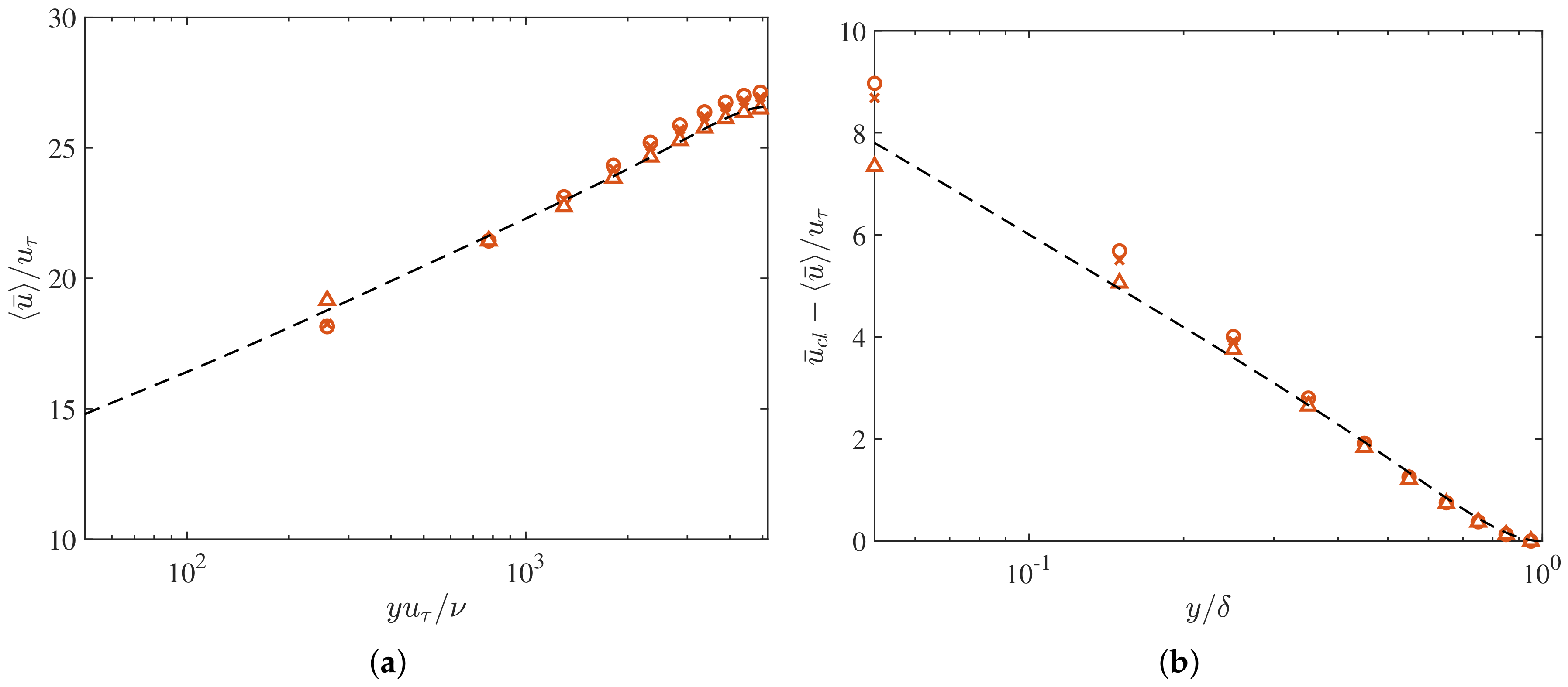
. The mean velocity profiles are shown in
Figure 1. The main difference is observed in the centerline velocity, where D-EV provides a better prediction compared to N-ZEV and N-EV (
Figure 1a). The three cases have little difference in the shape of the mean velocity profile in the outer region, as seen from the defect form of the mean velocity profile (
Figure 1b). This is consistent with previous observations that the boundary condition does not affect the outer region [
16,
31,
32]. The mean eddy viscosity for the three boundary conditions collapses in the outer region (
Figure 2), which is further evidence that the outer region is not affected by the wall boundary condition.
The discrepancy in the centerline velocity is due to the way the channel is driven. As the mean mass flow in the logarithmic region is constant, if the mean velocity profile in the logarithmic region (first 1 or 2 grid points off the wall) is underestimated, the mean profile is shifted up as is the case for the boundary conditions N-ZEV and N-EV. The Neumann boundary condition compensates for the missing wall stress by providing a very high streamwise velocity gradient at the wall (
Table 1), and the mean profile requires 1 or 2 grid points to counteract the steep gradient. In addition, the eddy viscosity close to the wall is estimated to be larger in the Neumann boundary condition cases (
Figure 2 and
Table 1), which increases the total SGS shear stress close to the wall, increasing dissipation in this region. While different methods of driving the flow may alleviate the mismatch in the centerline velocity (such as imposing the centerline velocity), this will shift the mean profiles of the N-ZEV and N-EV cases down in a way that will mean the velocity in the first two grid points will be underpredicted. This indicates that D-EV performs better compared to the other two boundary conditions closer to the wall, particularly in the first few grid-points off the wall and at the wall (
Table 1).
The resolved turbulence intensities in the form of root-mean-square velocity fluctuations are shown in
Figure 3a–c. Similar to the mean velocity profile, the turbulence intensities collapse for the three cases in the outer region, as expected from the collapse of the eddy viscosity in this region (
Figure 2). The main difference is observed in the near-wall region, where the D-EV case provides a better estimation of the turbulence intensities in the first two off-wall grid points. There is a marginal difference between the N-ZEV and N-EV cases, with N-EV providing slightly better estimation. Similar trends can be observed for the resolved tangential Reynolds stress,
(
Figure 3d). This difference can be attributed to the high streamwise velocity gradient at the wall for the Neumann boundary condition cases, which in turn elevates the eddy viscosity close to the wall (as seen in
Figure 2) and provides excessive dissipation close to the wall.
The effect of the eddy viscosity can be incorporated to study the turbulence intensities by accounting for the additional stress generated from
. If we take the Reynolds stress tensor for LES to be approximated as
we can compare the deviatoric part of
,
for the LES and DNS, where
is the Kronecker delta. The total tangential Reynolds shear stress
(
Figure 4d) shows that by including the effect of the SGS model, the missing stresses can be supplemented. The three diagonal components of
are shown in
Figure 4, which shows that for
and
, D-EV outperforms N-ZEV and N-EV, while results for
are mixed. Nevertheless, in most applications of WMLES, the statistics from the resolved quantities are taken as is without any additional consideration of the contribution from the SGS scales, and the results for
are meant for qualitative comparison.
3.1. Effect of Reynolds Number
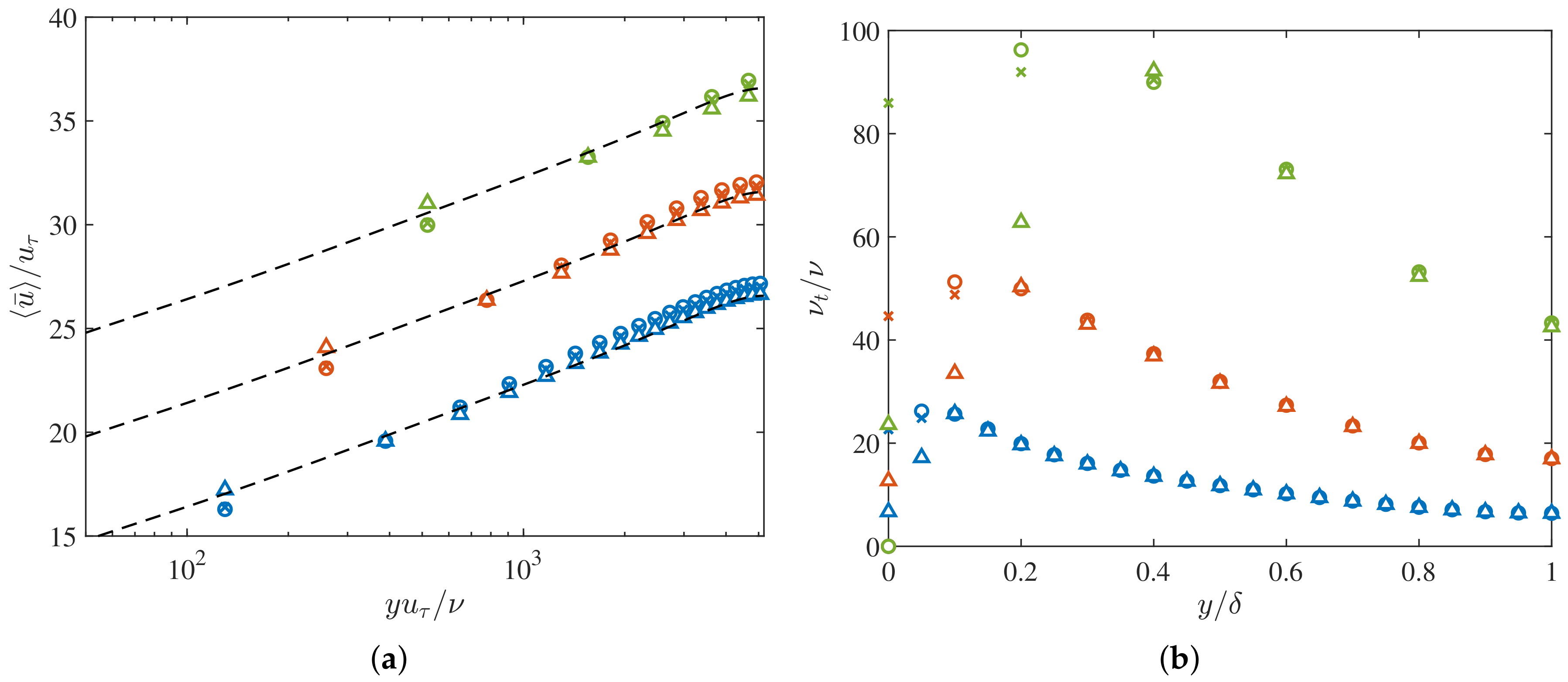
We compare the results of the WMLES with the three different boundary conditions at
,
and
at grid resolution
. The mean streamwise velocity profile is shown in
Figure 5a. Trends observed for the
case apply to higher Reynolds numbers, with D-EV providing the best results for the mean velocity profile. The overestimation of the mean velocity profile for the N-ZEV and N-EV cases, like the
case, seems to be due to the higher dissipation closer to the wall from the higher values of
in the first few off-wall grid points stemming from the higher values of
at the wall. The results for the turbulence intensities show similar trends as the
case for all Reynolds numbers (not shown), with D-EV showing better prediction of turbulence intensities in all three velocity components closer to the wall.
3.2. Effect of Grid Resolution
We compare the results of the WMLES with the three different boundary conditions at
at grid resolutions
,
, and
. The results obtained for the three grid resolutions are comparable for all the boundary conditions, with mean velocity profiles exhibiting similar trends for the baseline case (
Figure 6a). The eddy viscosity increases for coarser grids, as the SGS contribution increases (
Figure 6b). Regardless, the same observation that the eddy viscosity close to the wall is overestimated due to the large wall-normal gradient of the streamwise velocity at the wall holds for all grid resolutions. The results for the turbulence intensities show similar trends as the baseline case for all grid resolutions (not shown).
5. Conclusions
We introduced three different boundary conditions for applying wall shear stress derived from the mean stress-balance equations for a turbulent channel flow with a no-penetration boundary condition (). Depending on whether the eddy viscosity contribution at the wall is set to zero, the traditional boundary condition used for WMLES is either the Neumann boundary condition with zero eddy viscosity at the wall (N-ZEV) or the Neumann boundary condition with nonzero eddy viscosity computed from the SGS model (N-EV). However, the mean stress-balance equation can be also satisfied by changing the eddy-viscosity be nonzero at the wall while applying a Dirichlet boundary condition for the velocities, which we call the Dirichlet boundary condition with eddy viscosity augmentation (D-EV).
The D-EV boundary condition provides improved predictions of the mean velocity profile and turbulence intensities in the first few off-wall grid points compared to N-ZEV or N-EV. This improvement can be attributed to the limited wall-normal gradient of the streamwise velocity and a smaller eddy viscosity at the wall, leading to less dissipation in this region. As most SGS models are overly dissipative in the near-wall region [
36], the reduction in dissipation allows the D-EV to provide better statistics close to the wall. The three boundary conditions showed minor differences in terms of mean velocity and turbulence intensity prediction in the outer region, as expected.
The improved predictions in the first off-wall grid point for D-EV allow traditional wall models to be used with LES information from the first off-wall grid point without additional spatial or temporal filtering. This is contrary to N-EV, which is known to produce a log-layer mismatch when the first off-wall grid point is utilized as the matching location in WMLES. This was demonstrated using the equilibrium wall model [
14], which showed that D-EV enables the prediction of wall shear stress within 0.1% accuracy, unlike the case with N-EV, where the wall shear stress was underpredicted by 3%. The ease of implementation of D-EV together with its more accurate predictions in WMLES using the first off-wall grid point suggest that this boundary condition might be beneficial for flow over complex geometry where information farther away from the wall may not be readily available.


