1. Introduction
Non-Newtonian flows are present in many applications, such as mining, chemical engineering, environmental and civil engineering, etc. The non-Newtonian behavior can be generated by the internal structure of pseudohomogenous mixtures [
1,
2], such as in the case of foams, emulsions, suspensions, pastes, and polymer solutions, or by the particle interaction in heterogeneous mixtures, such as in mine tailings, mineral suspensions, wastewater sludges, and drilling muds.
The non-Newtonian rheological behavior is generally well described by the Herschel-Bulkley equation [
3]:
where
(Pa) is the shear stress,
(s
−1) is the shear rate,
(Pa) is the yield stress,
(-) is the flow behavior index, and
(Pa s
n) is the flow consistency index. It is worth pointing out that the flow consistency index has a noncoherent unit of measurement depending on
. With regard to the yield stress (
), it is the stress value at which the deformation begins: such a minimum stress is required to break the internal ‘structure’ of the mixture before any relative movement can occur. The HB rheological model describes both shear thinning (
< 1) and dilatant (
> 1) behavior [
2], and it is equivalent to the Bingham plastic model [
4] for
, the power-law model for
, and the Newtonian model [
5] for
and
. The HB model has been generally employed for its simplicity and ability to quantify the presence of yield stress and has been applied to several fluids, including sediment mixtures and sewage sludge [
6,
7].
Hallbom and Klein [
8,
9] found that the parameters of the HB model are variable functions of the shear rate [
10]. Thus, the measured parameters (
,
,
) are usually applicable over a limited shear rate range [
11]. Moreover, with reference to shear thinning fluids, according to the HB model, the apparent viscosity (
) tends to zero with an increasing shear rate. As slurries reach an asymptotic value of viscosity [
12], the HB model may imply inconsistencies for high shear rate flows, unless
(Bingham behavior) [
13,
14] is imposed.
Hallbom and Klein [
8] suggested that both HB and Bingham models are special cases of a more general rheological model (HK), expressed as:
where β is a dimensionless scaling factor and
is the infinite shear rate viscosity. The model, called “yield plastic”, is equivalent to the Casson model [
15,
16] for
, and it was shown to be able to describe the behavior of mineral suspensions over a wide range of shear rates without varying the physical parameters. Unlike the Herschel-Bulkley model [
3], the yield plastic parameters have rational units (i.e., Pa and Pa·s) [
17]. Moreover, the yield plastic model implies a finite value of the apparent viscosity at high shear rates and thus properly models the existing “post-Newtonian” region of non-Newtonian fluids [
18].
The standard procedure for the estimation of the rheological parameters is based on the use of a rheometer to carry out experimental tests [
19]. By applying and measuring wide ranges of stress, strain, and strain rate, it is possible to obtain the rheological curve and, by fitting, rheological parameters with most appropriate constitutive equation [
20]. This procedure is based on two important choices: the rheometer and the constitutive equation. In some cases, the choice of the rheometer can be problematic, since this instrument generally allows one to perform analysis only on a limited shear rate range [
8]. Moreover, in the case of a two-phase (liquid-solid) mixture with a solid density higher than liquid density, the sedimentation tendency (caused by gravitational force) may affect the results of the rheometer tests. For this reason, an experimental measurement on a pipe flow of the mixture can be preferred. Indeed, compared to the traditional viscometer experiments, a pressure pipe test ensures larger flow velocities and, consequently, a lower tendency for solid particle sedimentation [
21,
22]. As a result, the mixture can be treated for most purposes as a single-phase fluid. An additional advantage of the pressure pipe test lies in the possibility of exploring a full range of fluid dynamic conditions, including laminar, transitional, or turbulent regimes.
In the pressure pipe tests, once the appropriate constitutive equations are selected, the rheological parameters can result from the evaluation of head loss and discharge measurements [
23,
24,
25,
26]. Rabinowitsch (1929) and Mooney (1931) [
27,
28] described a method, widely used in the literature [
29,
30,
31,
32], based on the integration of the analytical laminar velocity distribution in the cross-section. Wilson and Thomas (1985) [
33] and Thomas and Wilson (1987) [
34] investigated the turbulent flow conditions of non-Newtonian fluids discussing the effects of the eddy size. According to the authors, the velocity profile of a non-Newtonian fluid can be split into three parts: (i) a viscous sublayer presenting an increased thickness compared to a Newtonian fluid, for the same wall shear stress, (ii) a turbulent zone, and (iii) a plug zone. By integrating the velocity profile in the cross-section, they found, for a Herschel-Bulkley fluid, a single relation between the rheological parameters of the fluid, the flow rate, the pipe friction losses, and the pipe diameter. Carravetta et al. (2016) [
35] recently developed a methodology for the estimation of the rheological parameters of HB fluids based on the equations proposed by Chilton et al. (1996) [
18] in laminar flow conditions and by Chilton and Stainsby (1998) [
21] in turbulent flow conditions.
In this study, the constitutive equations HB and HK are integrated over the cross-section to obtain a resistance formula in laminar flow, while the Wilson and Thomas method used to obtain a friction-flow relation in turbulent flow condition. As suggested by Thomas and Wilson (1987) [
34], the theory should be applied using as constitutive equation the rheological model by Herschel-Bulkley. In this study, such a theory in the literature is also extended to the Hallbom and Klein (2004) constitutive model. Based on these results, a new technique for estimating the parameters of HB and HK fluids in turbulent flow conditions is proposed. The new technique was applied to a complete set of experiments on a bentonite mixture, with the aim of determining the rheological parameters of both HB and HK models in laminar and turbulent flow conditions. By comparing the parameters obtained for both the rheological models, a better agreement between the model and the data was found with reference to the HK model, especially in the turbulent conditions.
Finally, a numerical model of dam-break propagation within a non-Newtonian fluid was applied by using the rheological parameters resulting from both HB and HK models. The differences in the process evolution arising from the application of either the HB model or HK model are discussed.
3. Friction Flow Model in Turbulent Flow Conditions
The friction flow model in turbulent conditions has been deeply investigated by Wilson and Thomas (1985) [
33] and Thomas and Wilson (1987) [
34]. According to the authors, the thickness of the viscous sublayer (δ
v) is proportional to the area ratio
, defined as the ratio between the area below the non-Newtonian rheogram (i.e., dashed area in the left plot of
Figure 2) and the area below the Newtonian rheogram, for a given wall shear rate and the corresponding wall shear stress (i.e., dashed area in the right plot of
Figure 2).
The expression of
is given by Equation (11):
With reference to
Figure 2, the slope of the Newtonian rheogram is the apparent viscosity, and as previously mentioned, it is evaluated by the following expression:
The velocity within the viscous sublayer (
) is a linear function of the distance from the wall (
) according to the following expression:
where
is the density,
is the distance from the wall, and
is the shear velocity (
).
The intercept with the logarithmic profile of the turbulent layer is given by:
The thickness of the viscous sublayer (δ
v) depends on
according to the following expression:
Outside of the viscous sub-layer, the velocity of the turbulent flow (
) varies logarithmically with
, as follows:
In the case of
, the previous relations are valid for a Newtonian fluid. With reference to Equation (16), the plug velocity (
) in turbulent condition can be therefore expressed as:
With regard to the mean velocity
, it should be obtained by a numerical integration of the velocity profiles resulting from Equations (14), (16), and (17), as follows:
By solving Equation (18), hence:
where
is the mean velocity for equivalent Newtonian flow (i.e., the Newtonian flow presenting the same wall shear stress
) with the secant viscosity
, whereas the term
takes into account the blunting of the velocity profile due to the yield stress and is expressed as follows [
33]:
With regard to
, its expression varies according to the viscosity model. In case of fluids modeled according to Herschel-Bulkley [
3] (HB), the following expression proposed by Thomas and Wilson (1987) [
34] can be used:
Thus, Equation (19) is the resistance formula, relating and , in turbulent flow conditions.
Regarding fluids modeled by Hallbom and Klein [
8] (2009), the value of
should result from Equation (22), which cannot be analytically solved though.
Hence, the value of in HK fluids necessarily results from the numerical solution of the integral in Equation (22). Thus, even in turbulent flow, an explicit resistance formula does not exist for HK fluids, but the relation between and must be numerically obtained.
4. Experiments
Extensive pressure pipe tests were performed on a recirculating pipe using two different mixtures: a natural Bingham-plastic mixture and a bentonite mixture.
Steady state experiments were performed on three different pipes: (1)
= 2.91 mm,
= 1.47 m; (2)
= 18.05 mm,
= 5.42 m; (3)
= 25.82 mm,
= 5.88 m) with different volume concentrations of the mixtures. The pipe lengths were verified to be by far greater than the hydrodynamic entry region, which is approximately equal to
in turbulent flow condition [
36] and around
in laminar flow condition [
37]. In
Table 1, the total number of samples (
) is presented for each combination of diameter (
) and concentration value (
). Head losses
and discharge
were measured, respectively, by differential manometers and volumetric method. The details of the experimental facility can be found in Carravetta et al. (2010) [
38].
By increasing the flow rate, laminar, transitional, and turbulent flow conditions were observed. Since in the case of Bingham-plastic natural mixture few data were obtained in laminar flow conditions due to the sedimentation tendency of the suspended material, in this study, only the data resulting from bentonite mixture were used. This mixture was composed by salt water (3%), as well as bentonite at different values of volume concentration c (i.e., 0.0144; 0.03; 0.054; 0.075; 0.089; 0.12; 0.15; 0.18; 0.21; 0.25).
The experimental values of wall shear stress and mean velocity were calculated by means of Equations (23) and (24).
The experimental errors involved in the estimation of
and
approximately amount to 1.5% and 1%, respectively.
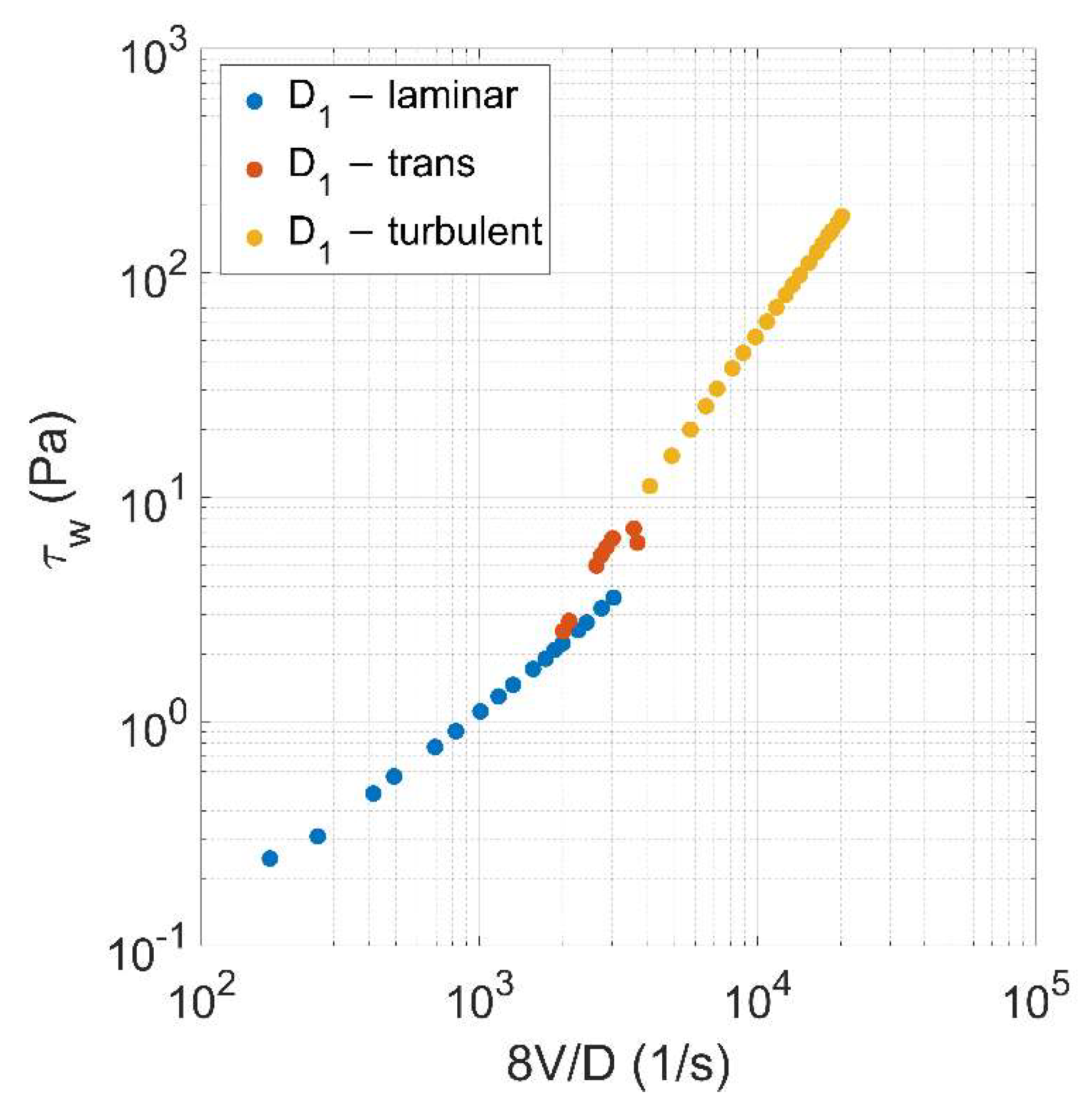
Figure 3 shows the log-log plot of experimental wall shear stress against
, obtained for a diameter equal to 2.91 mm and a concentration as 0.0144. According to
Figure 3, the points lie in three different regions depending on the flow regime (i.e., laminar, transitional, and turbulent), as first pointed out by Bowen (1961) [
39].
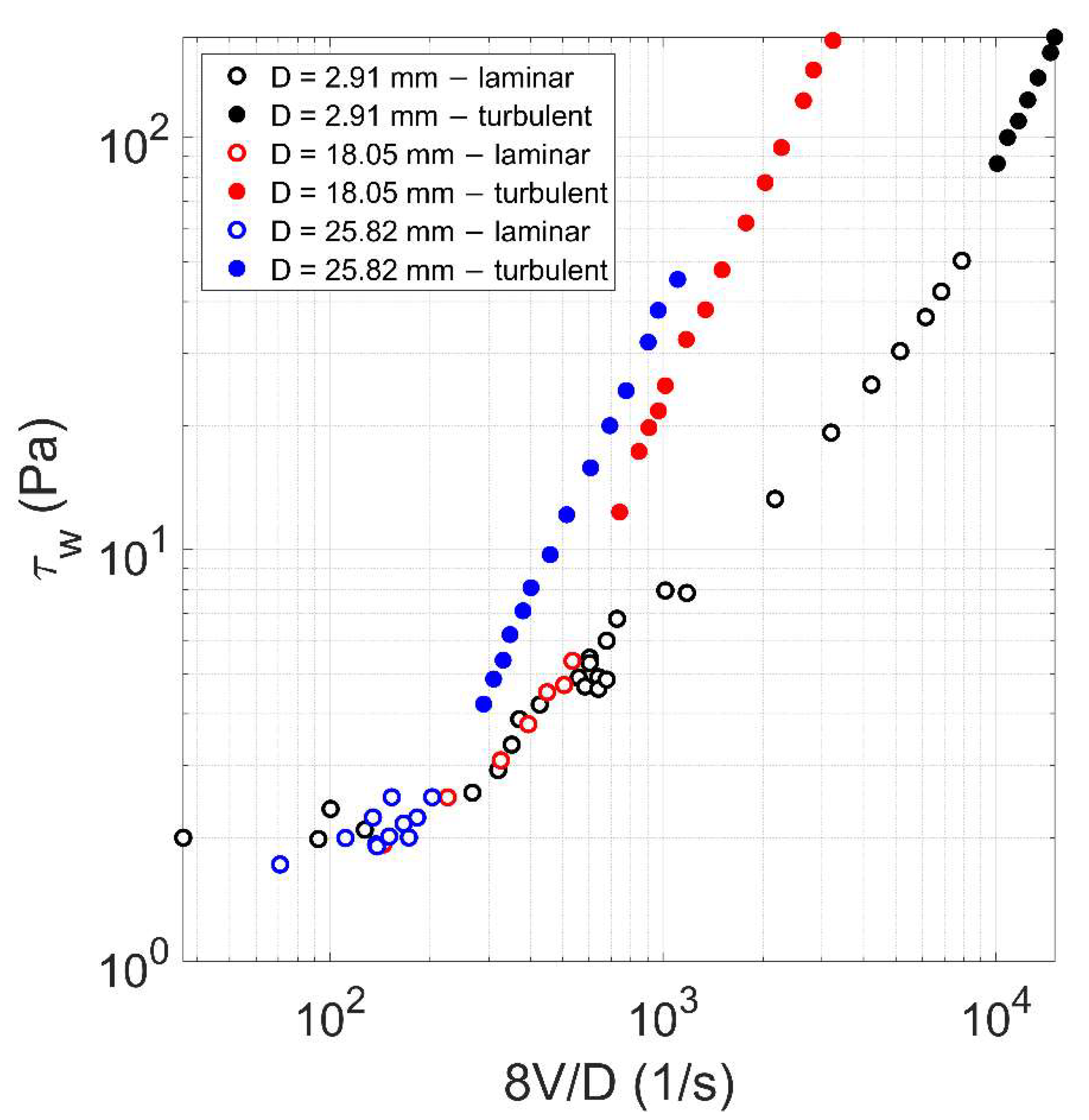
Figure 4 shows the log-log plot of the experimental wall shear stress against
for different diameters and fixed concentration (0.0144). With regard to the transitional flow regime, it was eliminated and is not considered any longer in this study owing to the hysteretic behavior (as shown in
Figure 3). With reference to
Figure 4, three turbulent branches can be observed, corresponding to three different pipe diameters, the larger one corresponding to the left line. The slopes
of the three turbulent branches are equal to: (i)
= 1.71 for
= 2.91 mm; (ii)
= 1.74 for
= 18.05 mm; and (iii)
= 1.76 for
= 25.82 mm. The difference in slope between the three branches is significantly small and could be due to experimental uncertainties: in this case, in the dependence of
on
, the exponent of
may be not dependent on
, in turbulent flow condition. With regard to the laminar regime, due to the dependence of the resistance term on
according to Equation (6), which is valid for HB fluids, the laminar flow data result to lie on the same curve, regardless of the pipe diameter. As demonstrated by Rabinowitsch (1929) [
27] and Mooney (1931) [
28], this behavior happens for any time-independent fluid, regardless the chosen rheological model.
5. Optimization Process
In order to obtain the best triad of rheological parameters (
for Herschel-Bulkley model [
3];
for Hallbom and Klein model [
8]) for each concentration value, an optimization procedure was performed by means of the MATLAB (R2019b, MathWorks, Inc., Natick, MA, USA) optimization toolbox [
40]. The objective function of the model consists of the minimization of the average error
) in the prediction of the mean velocity, as shown in Equation (25).
where the predicted mean velocity
was evaluated according to both Herschel-Bulkley [
3] and Hallbom and Klein (2009) models [
8] previously presented.
The values of rheological parameters (
for Herschel-Bulkley model [
3];
for Hallbom and Klein model [
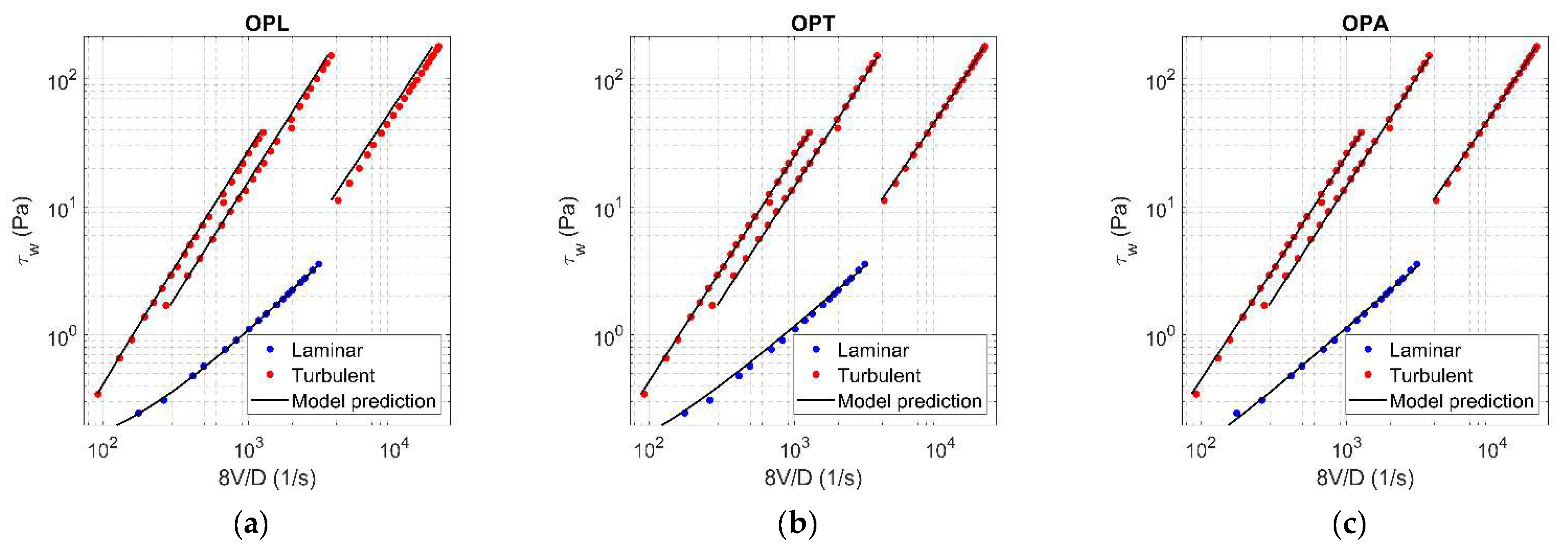
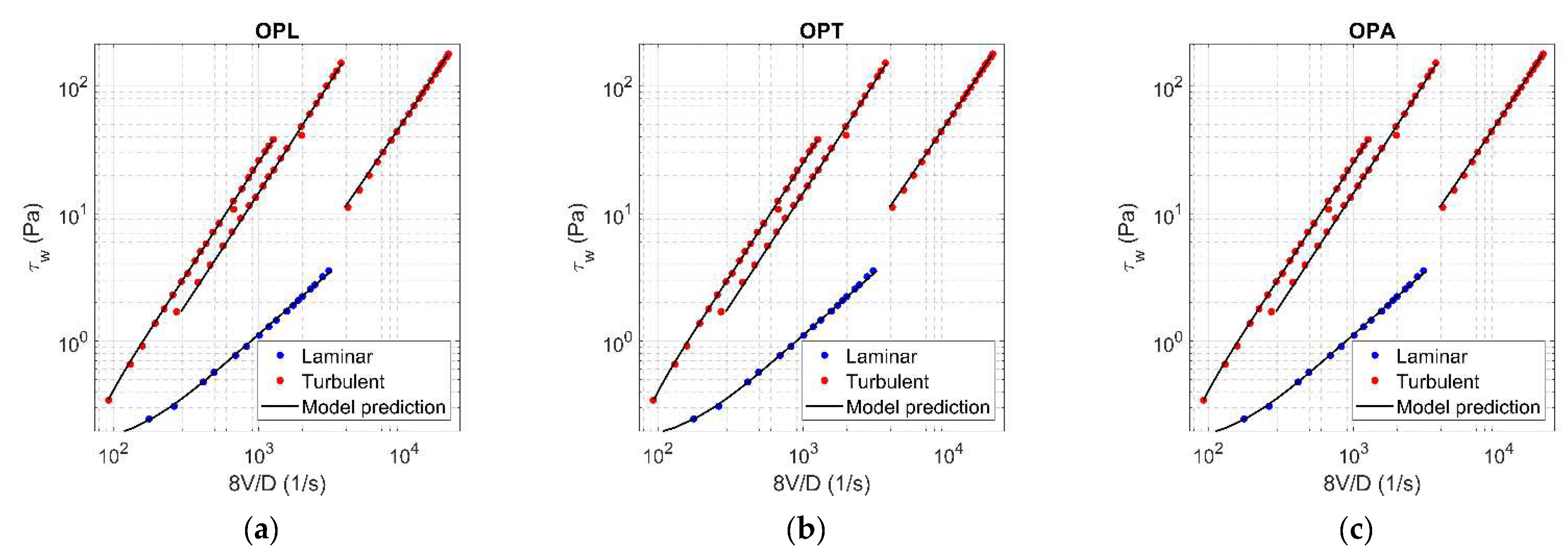
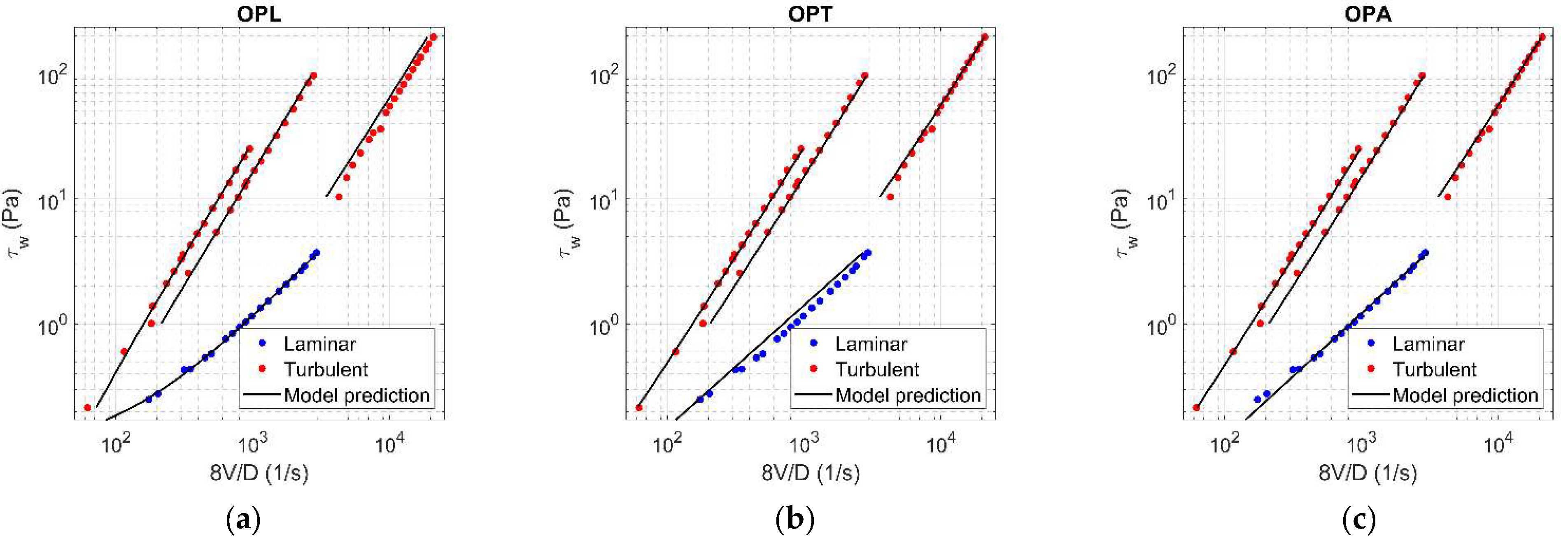
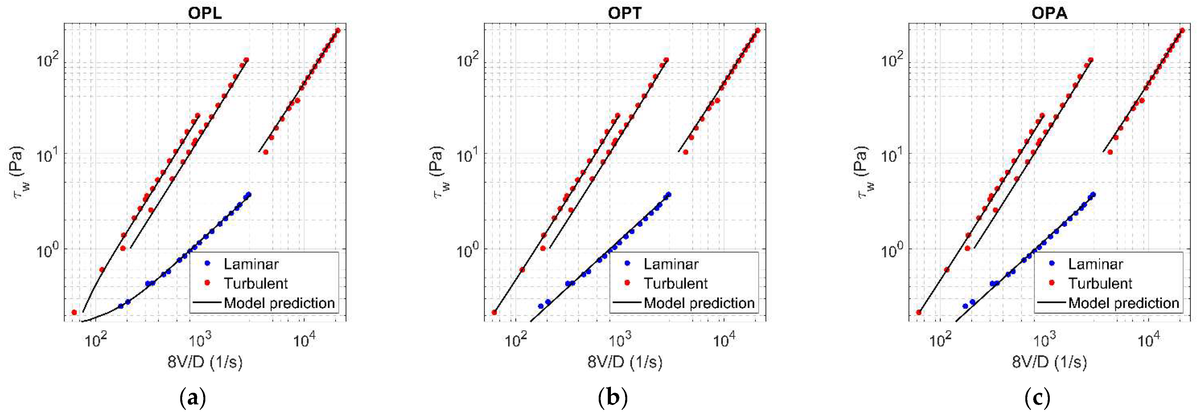
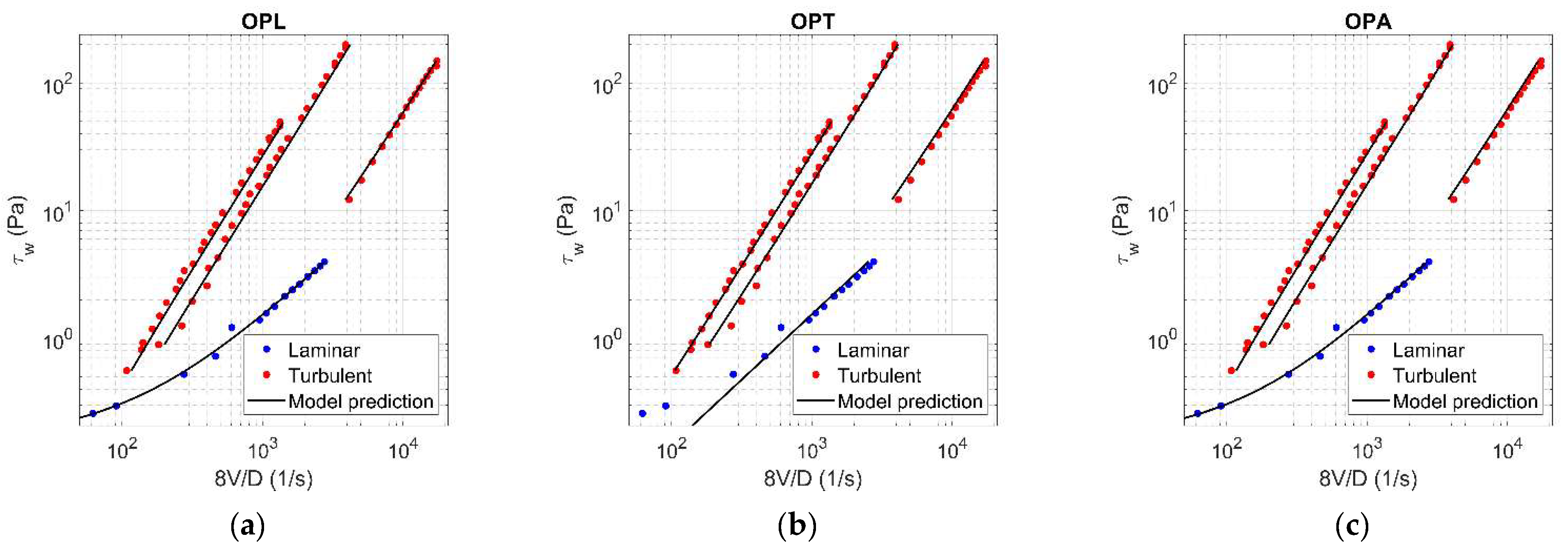
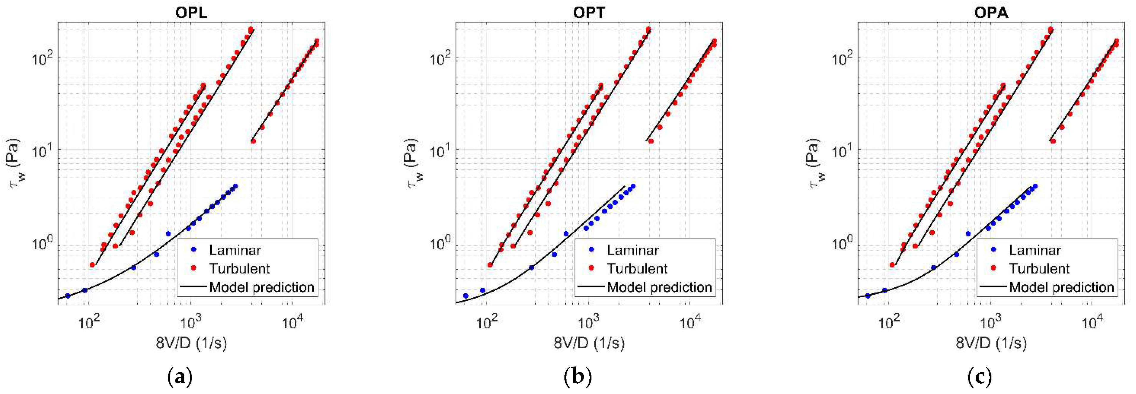
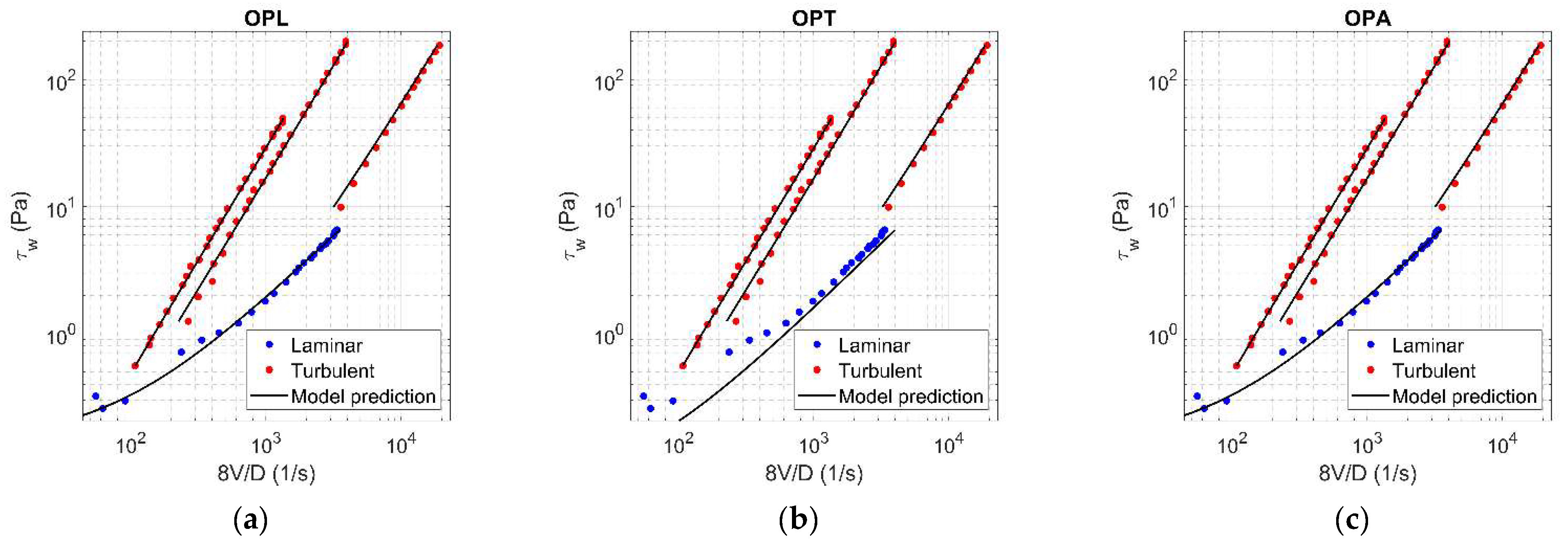
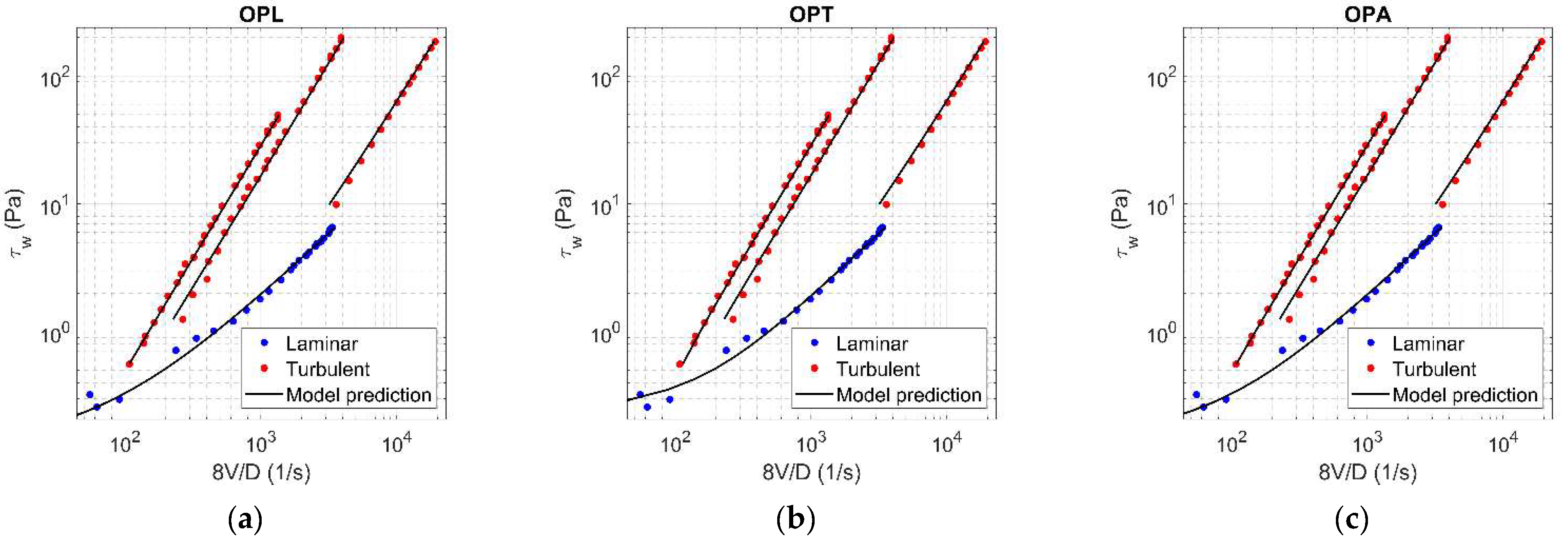
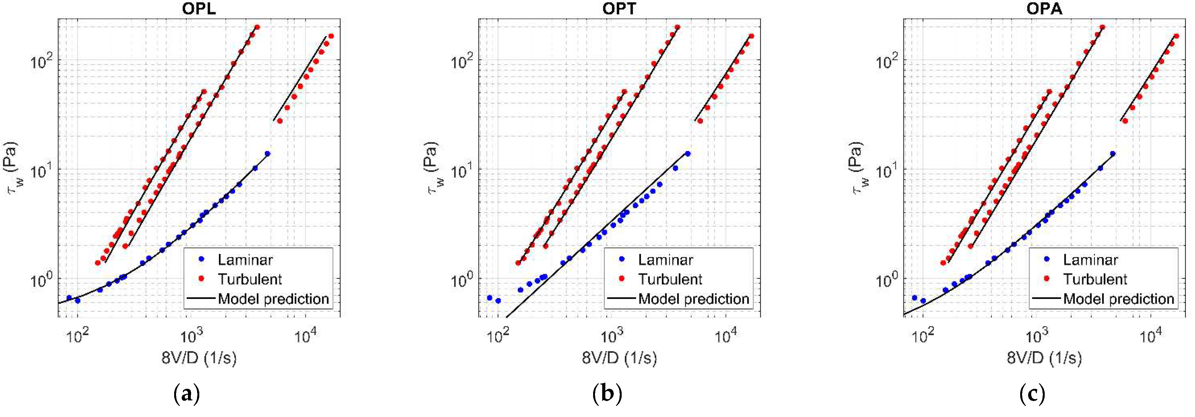
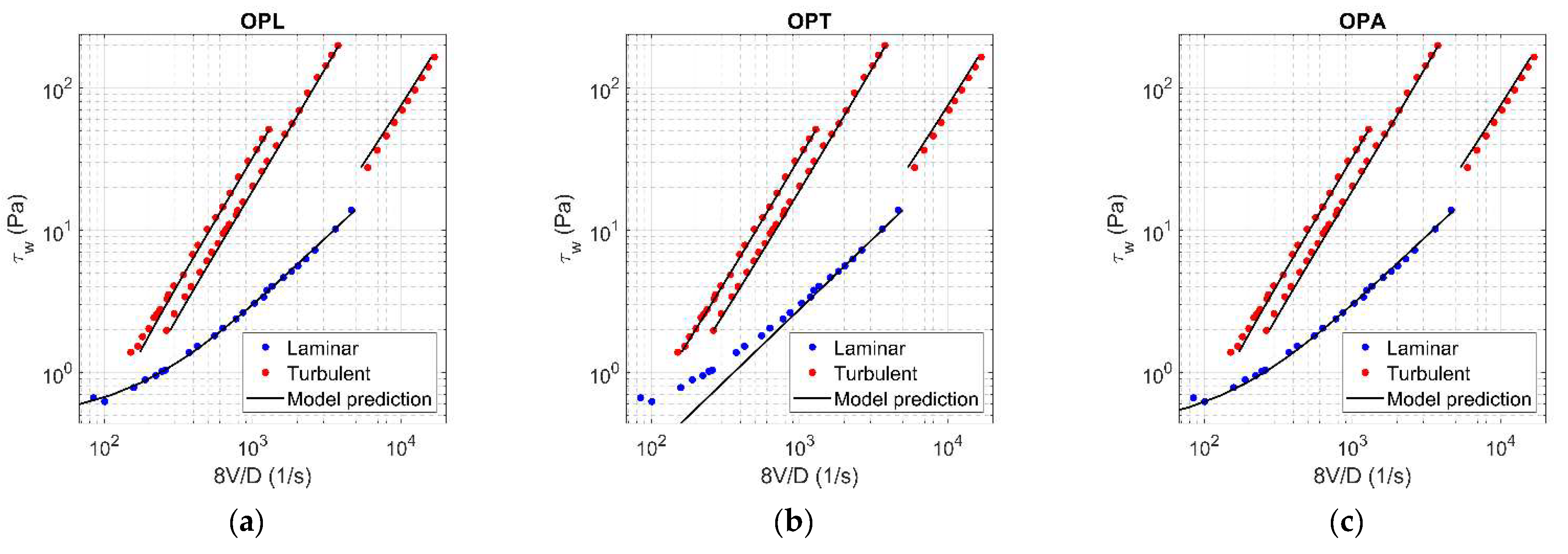
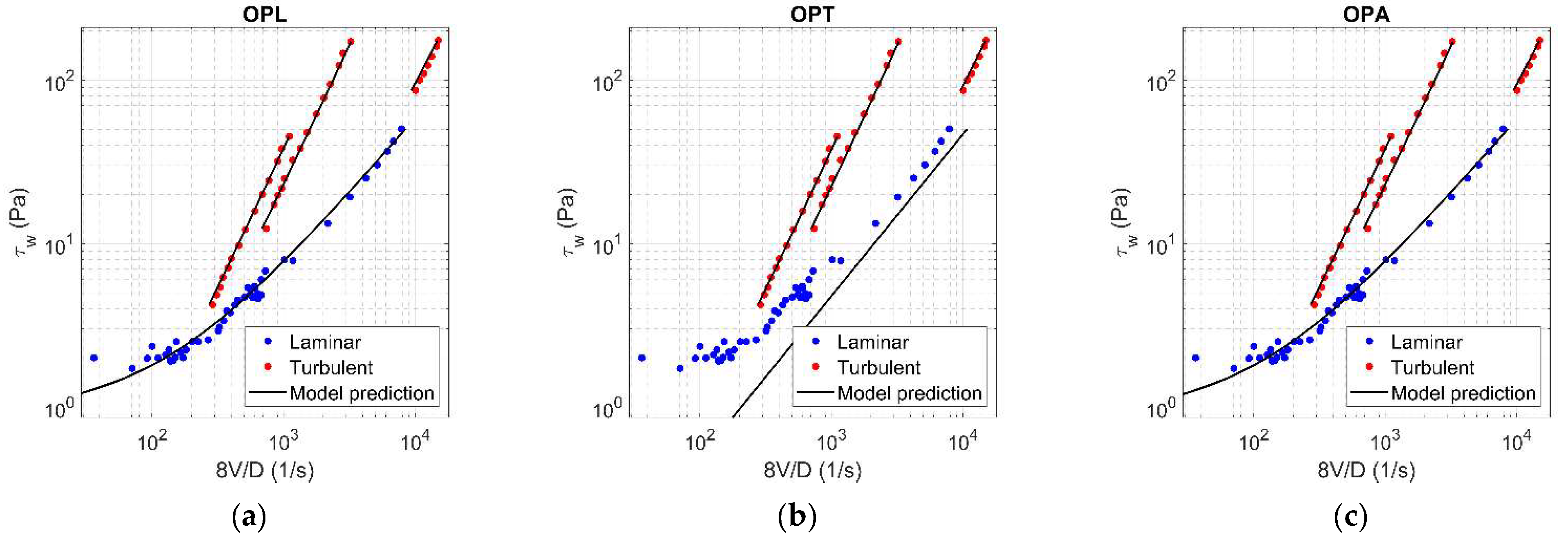
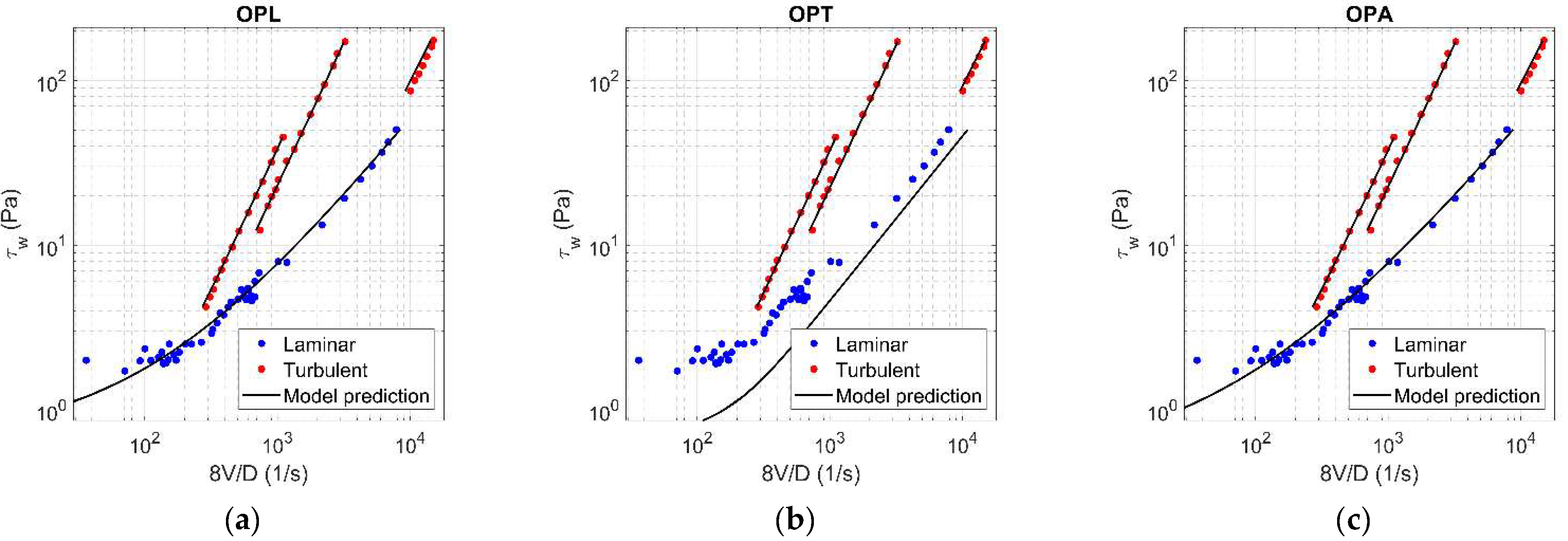
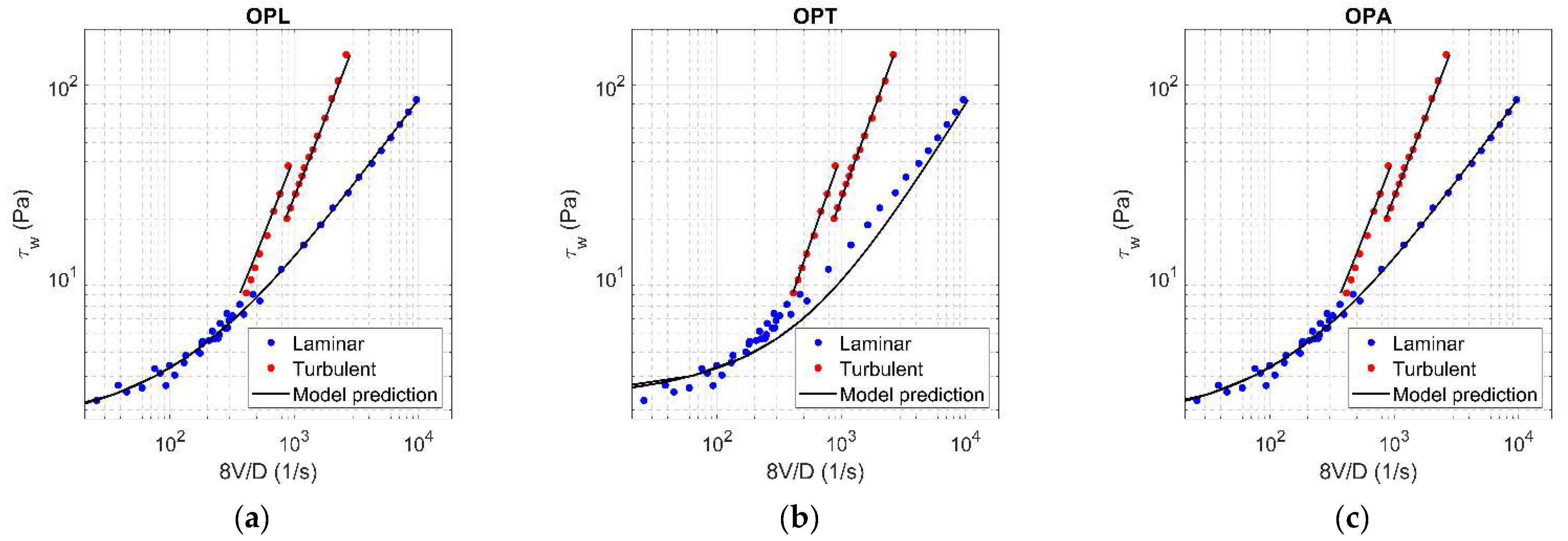
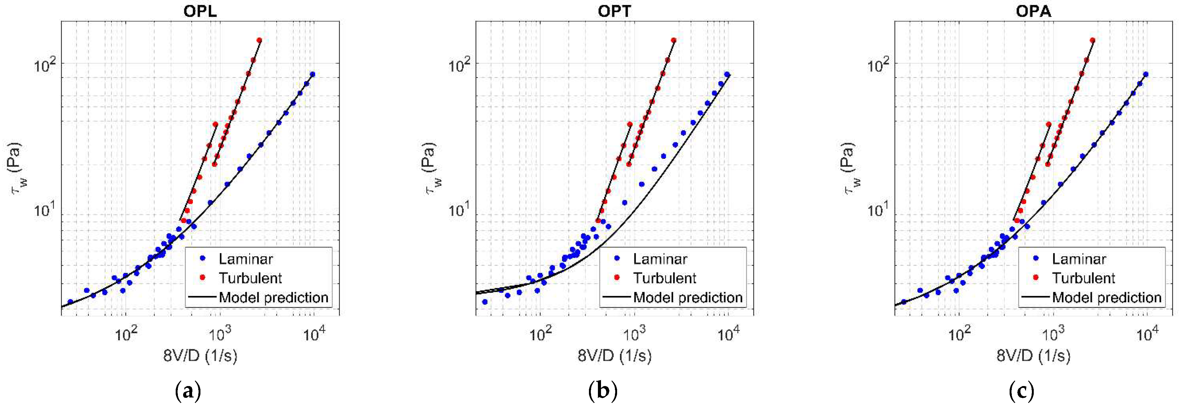
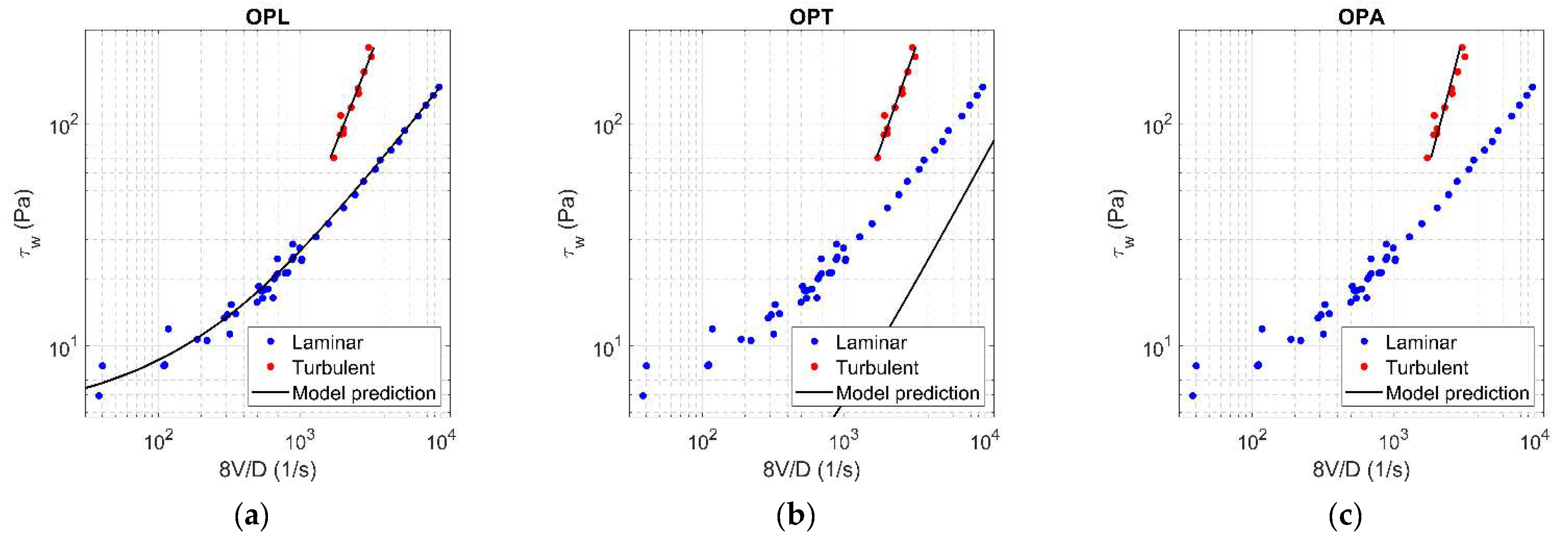
8]) were assessed for each concentration by applying the optimization procedure, using alternately laminar data (OPL), turbulent data (OPT), and finally all data (OPA). With reference to
= 0.0144,
Figure 5 and
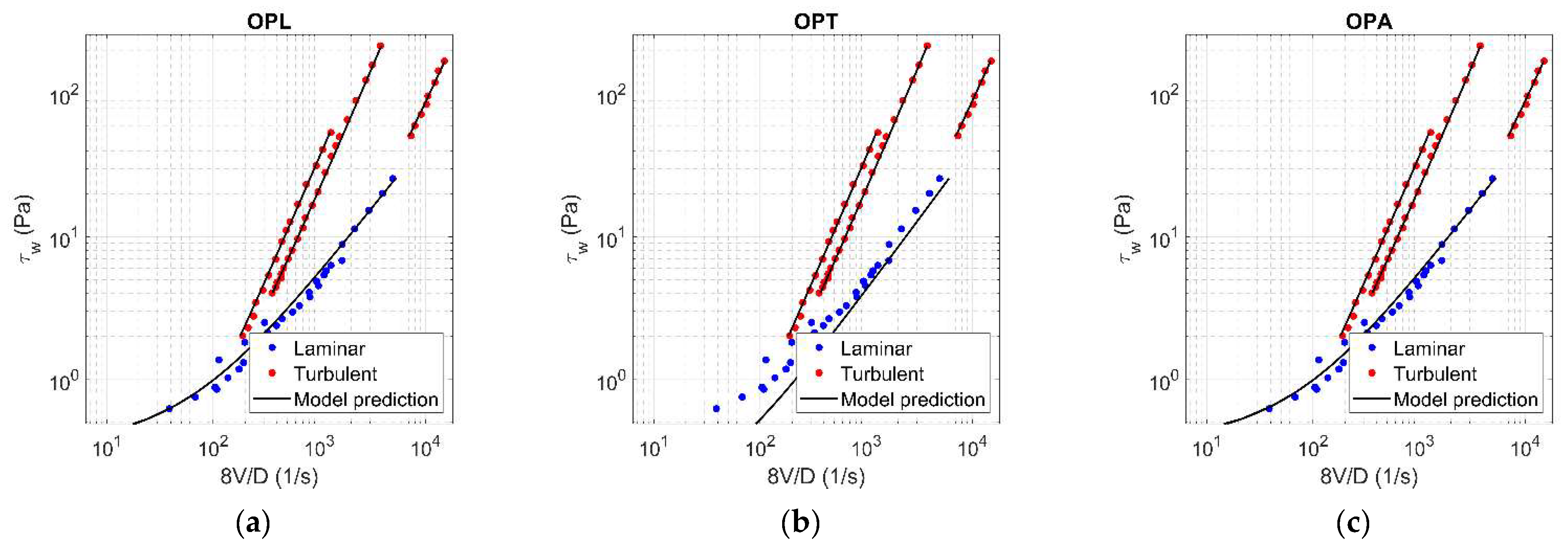
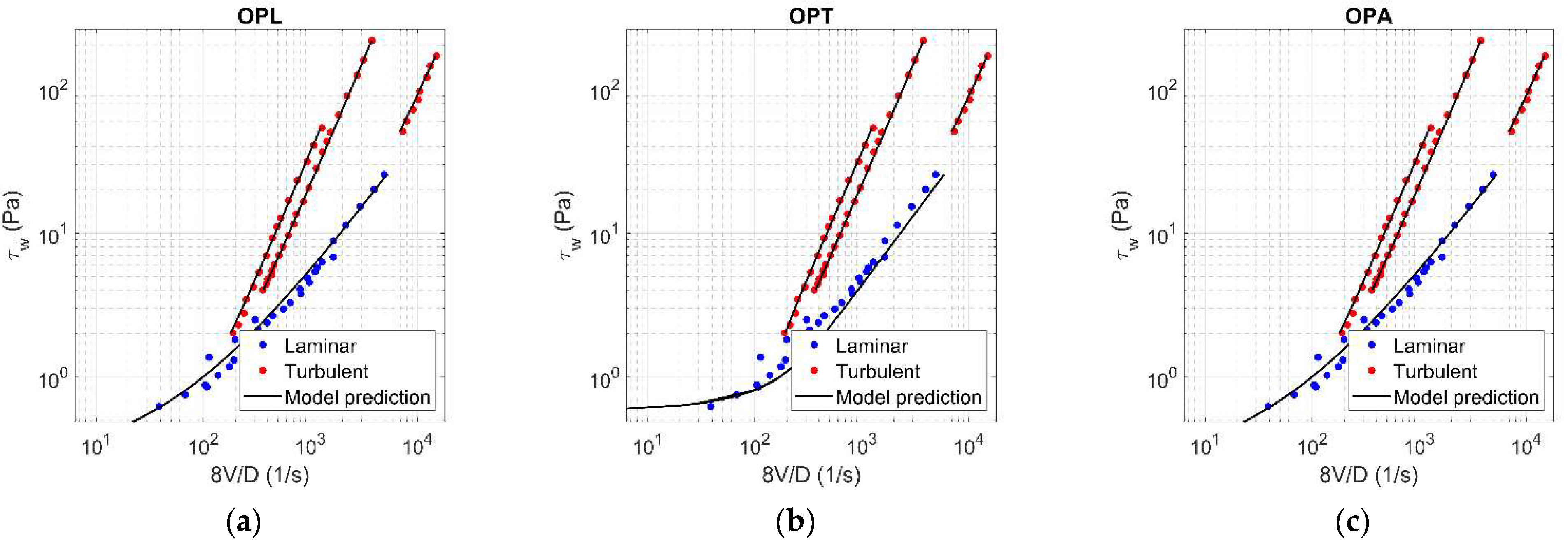
Figure 6 show the results of OPL (a), OPT (b), and OPA (c) when HB and HK, respectively, are chosen as rheological models. The results related to the other concentration values are reported in
Appendix A.
5.1. Results of Optimization on Laminar (OPL) and Turbulent (OPT) Data
The values of the rheological parameters obtained by fitting laminar data (OPL) are reported in
Table 2 and
Table 3, with reference to an HB and HK fluid, respectively. The objective function of OPL was
in laminar conditions (
). The average error in predicting the flow behavior was also evaluated with reference to the turbulent data (
) and all data (
). According to
Table 2 and
Table 3, the quality of the optimization for HB or HK fluid was the same, being the average errors on laminar data (i.e.,
, which is the objective functions in OPL) significantly close. However, the average errors in predicting the flow behavior with reference to both turbulent and all data result in differing among the constitutive models.
The values of the rheological parameters obtained by performing the optimization on turbulent data (i.e., OPT) are reported in
Table 4 and
Table 5, with reference to an HB and an HK fluid, respectively. The objective function of the optimization was
in turbulent conditions (
). The average error in predicting the flow behavior was also evaluated with reference to the laminar data (
) and all data (
).
According to the results, since the average errors on turbulent data (i.e.,
, which is the objective function in OPT) are very close, the quality of the optimization for an HB or an HK fluid is essentially the same. However, the average errors in predicting the flow behavior with reference to both laminar and all data result in differing among the constitutive models. Finally, due to the dispersion of the experimental points in laminar condition for high values of concentration (see figures in
Appendix A), the error of OPL and/or OPT on laminar data (i.e.,
) can be even greater than the error associated with turbulent points (
).
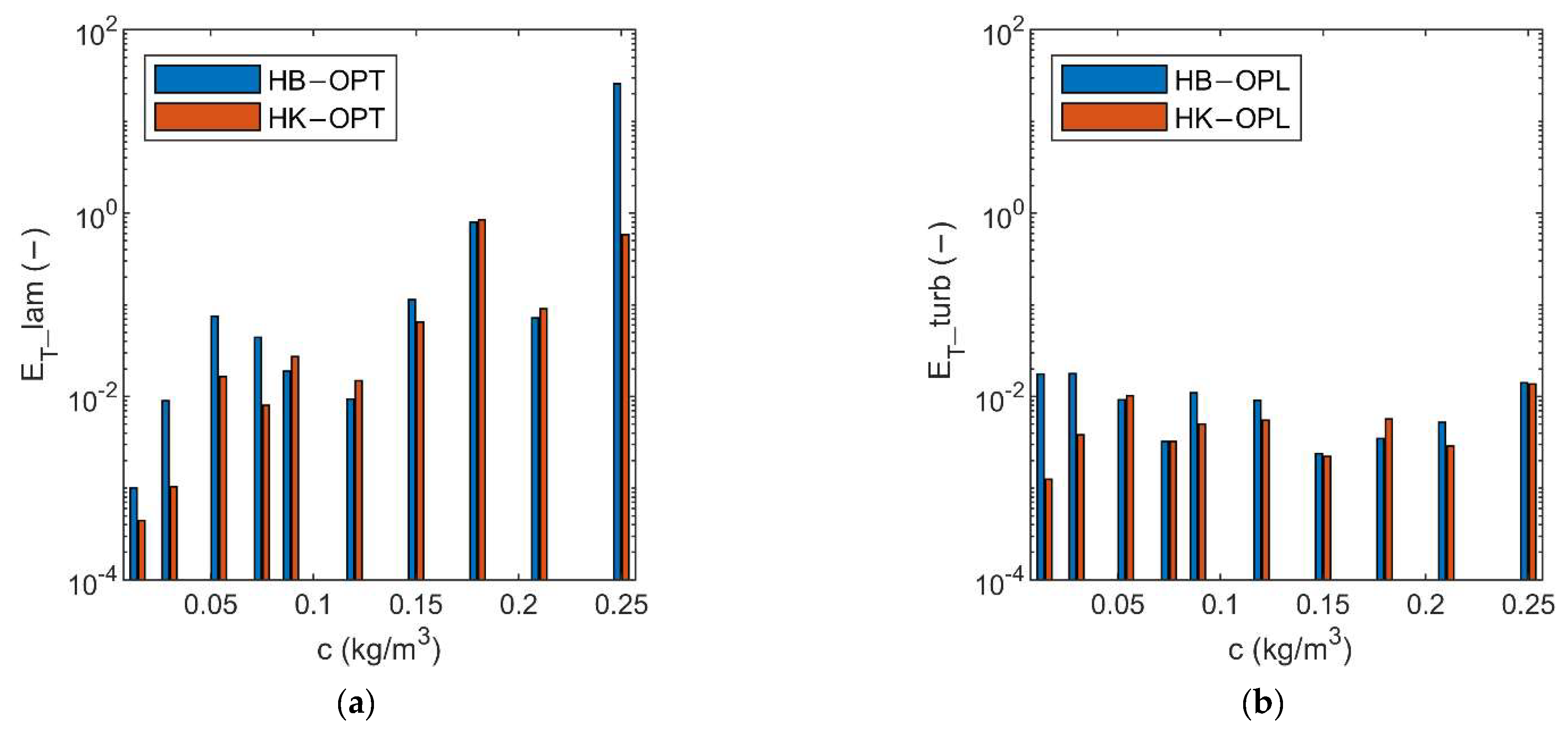
Figure 7 shows, for both HB and HK models, the average errors in predicting laminar velocities in OPT (i.e., when turbulent data are employed within the optimization—see left plot), as well as the average errors in predicting the turbulent velocities in OPL (i.e., when the optimization is performed on laminar measurements—see right plot). According to
Figure 7, the average error associated to OPT is overall larger than the error generated by OPL and such error results increase with increasing the value of the concentration
. As a consequence, the optimization performed on laminar data (OPL) may achieve more meaningful results. On the other hand, the measurements in laminar conditions are not always available due to the sedimentation tendency of the mixture. However, with reference to OPT, since the HK model exhibits a better performance in terms of average errors, it can be preferred over the HB model.
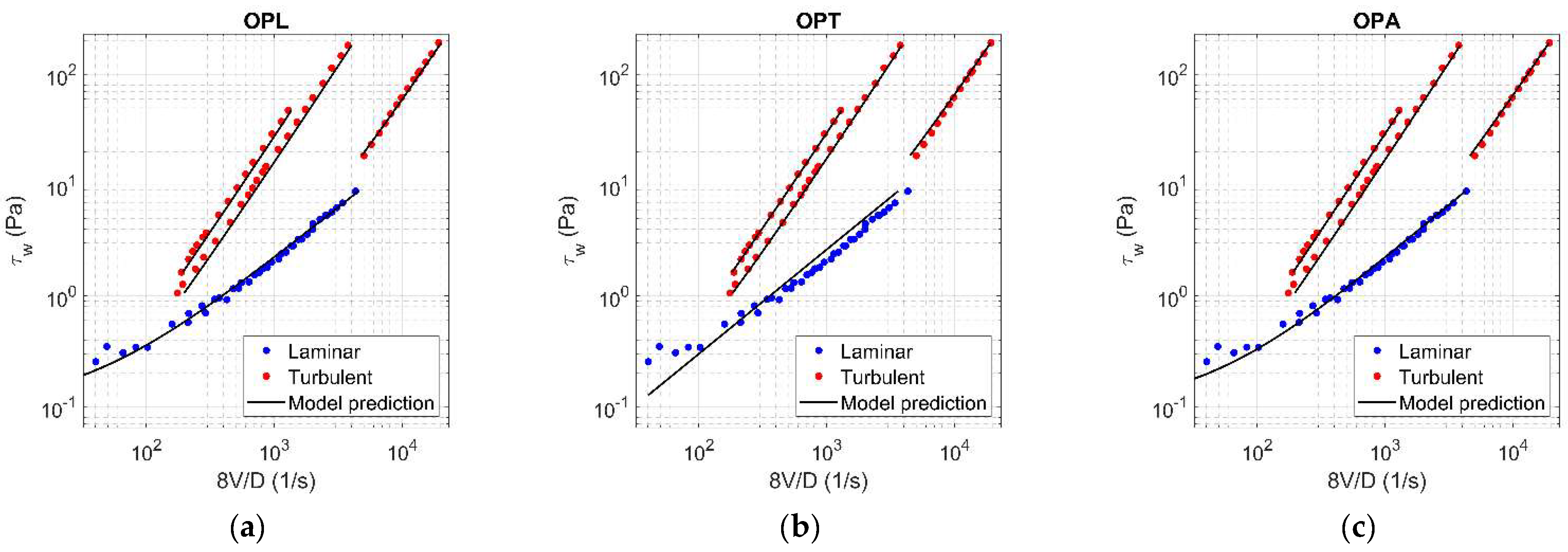
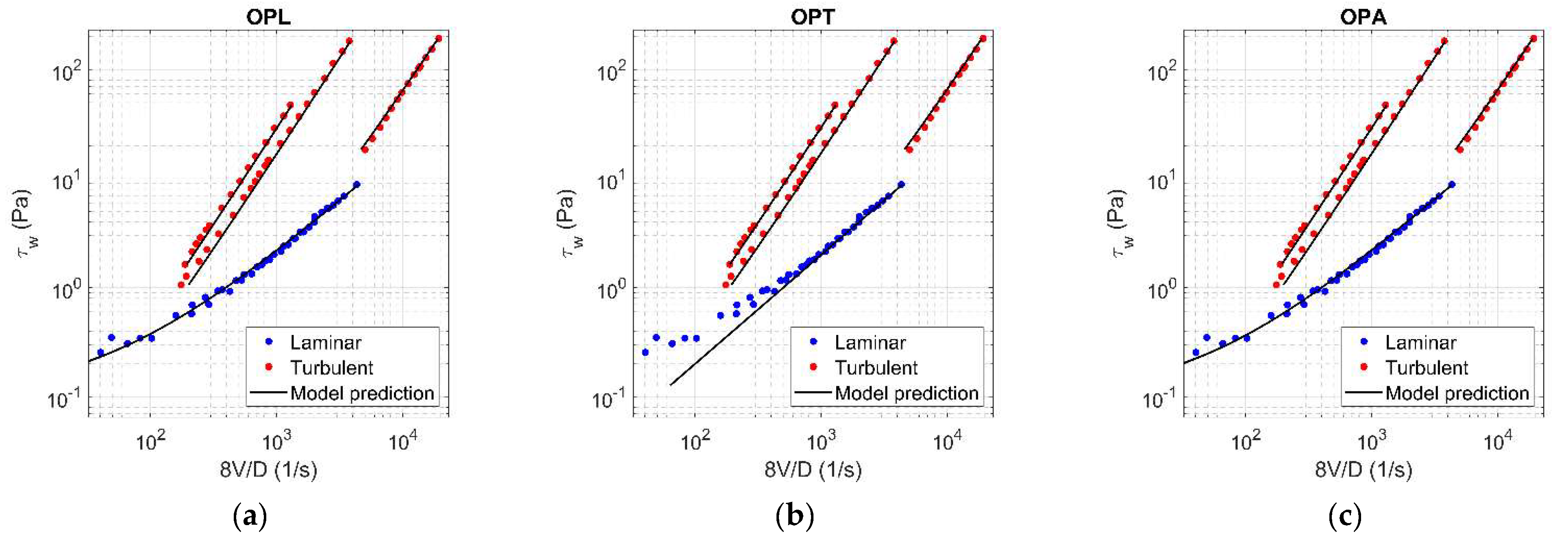
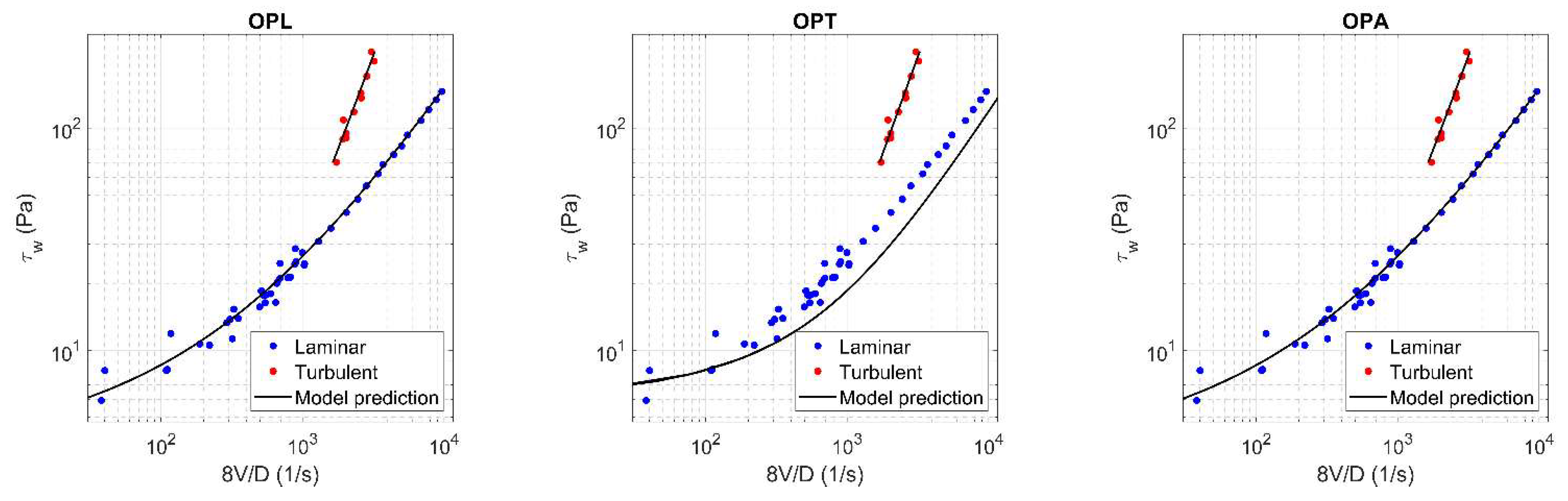
5.2. Results of Optimization on all Data (OPA)
The values of the rheological parameters obtained by an optimization on all data are reported in
Table 6 with reference to an HB fluid and in
Table 7 with reference to an HK fluid. The optimization was performed by using as objective function
. However, the average errors affecting the models are also given with reference to laminar and turbulent data. According to the values in
Table 6 and
Table 7, OPA results in smaller values of average errors, when compared with OPL and OPT.
5.3. Final Considerations on the Optimization
When a comprehensive set of data is available, both Herschel-Bulkley [
3] and Hallbom-Klein [
8] models could be used to assess the rheological parameters of a mixture. In many cases, only laminar data or turbulent data are available: the first situation occurs when the tests are performed by the use of a rheometer, whereas the latter is typically observed when pressure pipe tests are necessary to avoid sedimentation of the suspended particles of the mixture. In both cases, by considering a fluid modeled according to Hallbom-Klein [
8], the prediction of the flow behavior in a different hydrodynamic regime can be made in a much safer way, as proven by this study.
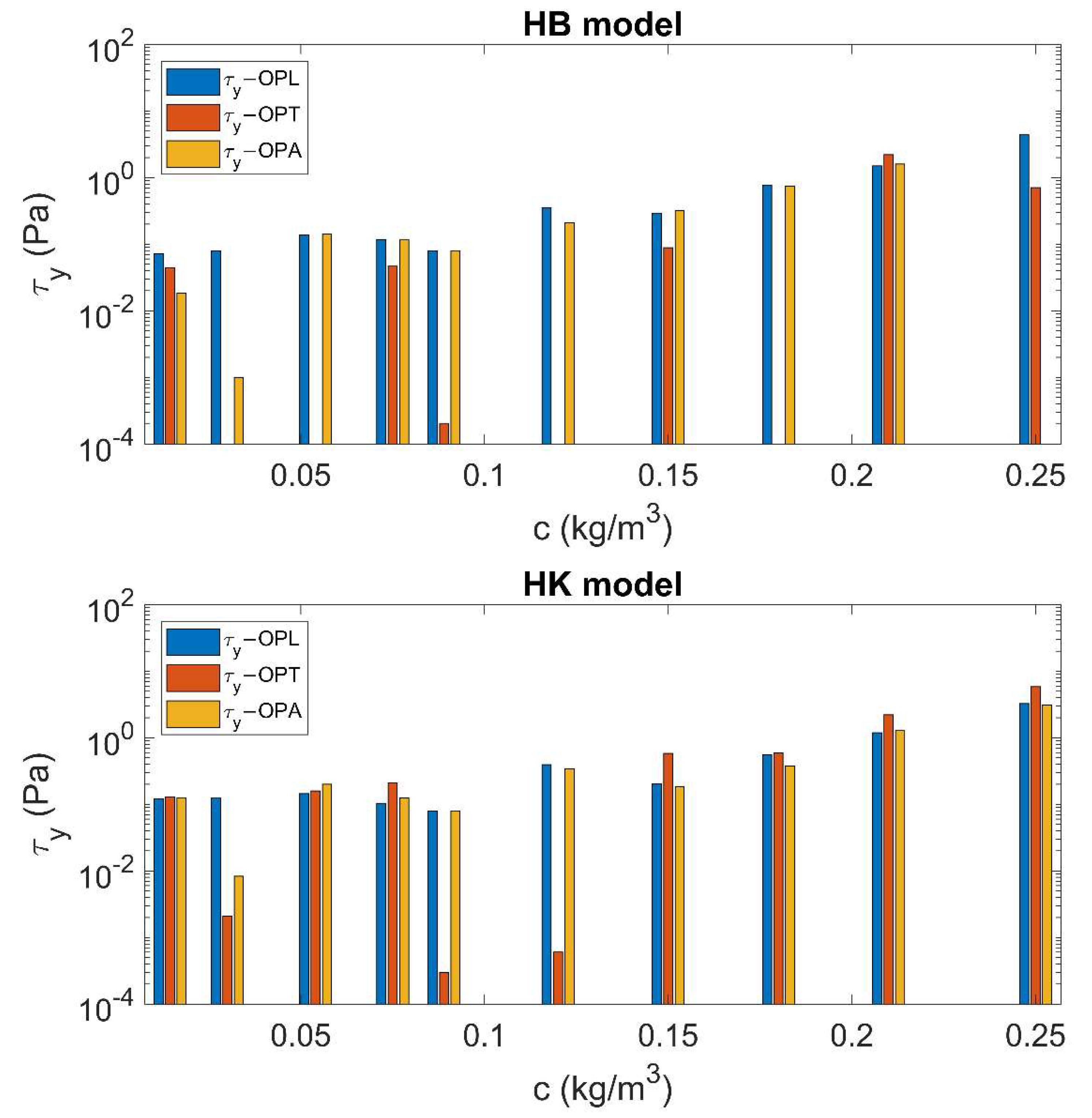
Figure 8 shows the values of
(that is the parameter in common between the two rheological models) obtained by OPL, OPT, and OPA for both HB and HK fluids.
With reference to
Figure 8, except for a few values of
,
resulting from OPL, OPT, and OPA is essentially the same when the fluid is modeled according to HK. Conversely, when HB is used as rheological model, the values of
significantly differ each other. Thus, unlike the HB model, HK is capable of fitting the experimental data in OPL, OPT, and OPA with a slighter variation of the parameters, further proving its internal consistency.
6. Engineering Implication: A Simple Dam-Break Example
The propagation of the flow after a dam-break event [
41] has been considered as a practical example to highlight the implication of the choice of the rheological model in terms of flow modeling [
42,
43,
44].
The case study consists of an instantaneous dam break in a 1-D prismatic and horizontal channel for a semi-infinite reservoir. The initial velocity is zero, while the initial depth is
. The 1-D shallow water equations that describe the motion of the fluids are the following:
where
is the fluid depth,
is the flow mean velocity,
the gravity acceleration,
the channel slope (zero in the case study),
is the resistance force for unit of weight, and (
) are the space and time coordinates. Harten-Lax-van Leer (HLL) finite volume method [
45] was used to solve the problem, where the source term was modeled by an explicit backward-time scheme. The simulations consider either laminar or turbulent flow conditions. For the calculation of the wall shear stress that appears in the source term, in turbulent flow condition, the abovementioned Thomas and Wilson theory [
34] was used, whereas for the laminar flow, a numerical integration of the constitutive equation over the flow depth was performed. The time-step
was chosen in order to keep the Courant number significantly lower than 1, i.e.,
, where
is the space discretization. For further information about the numerical method, please see [
46,
47]. In this simulation, the OPL parameters for a sediment concentration equal to 0.25 were considered.
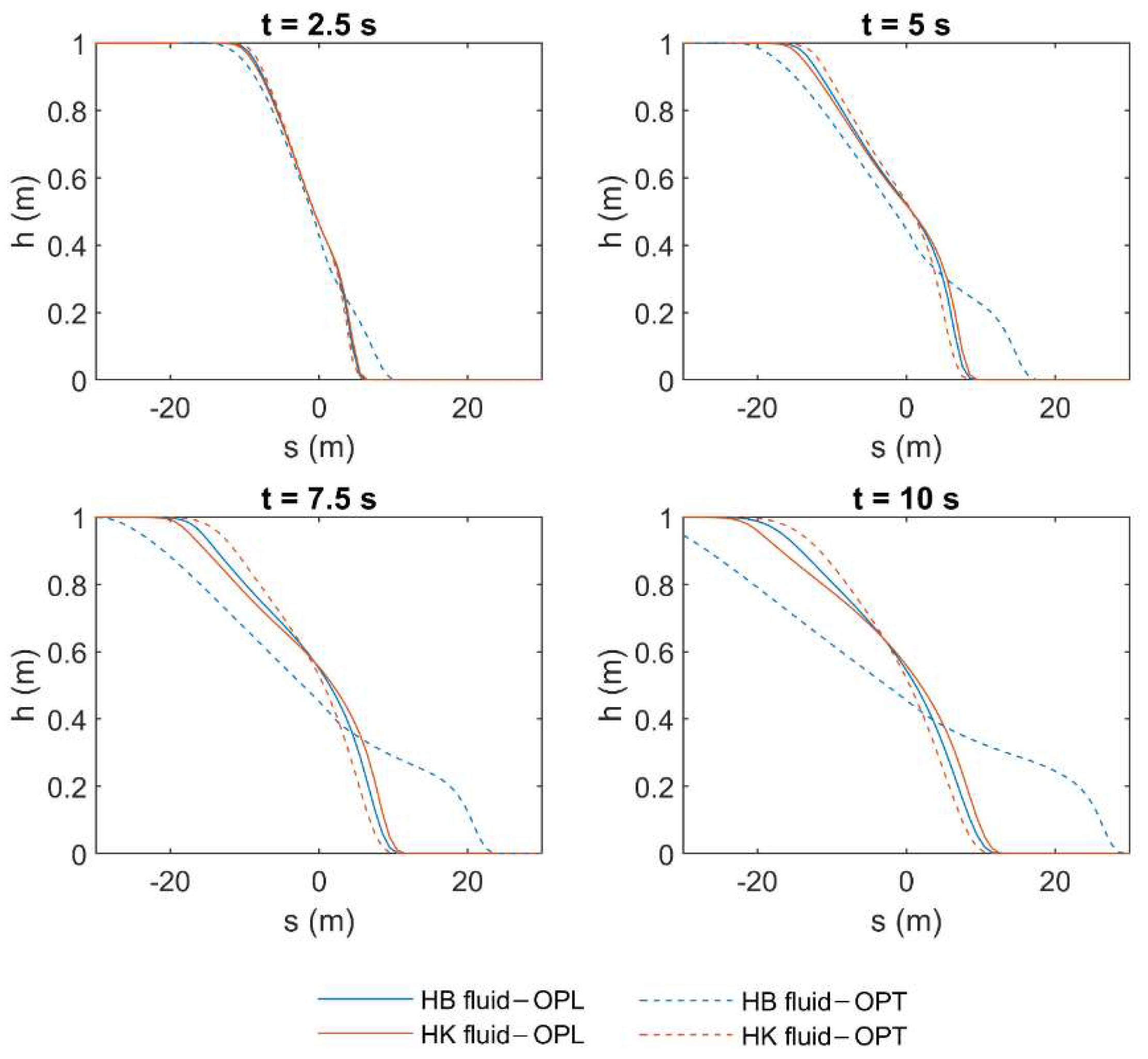
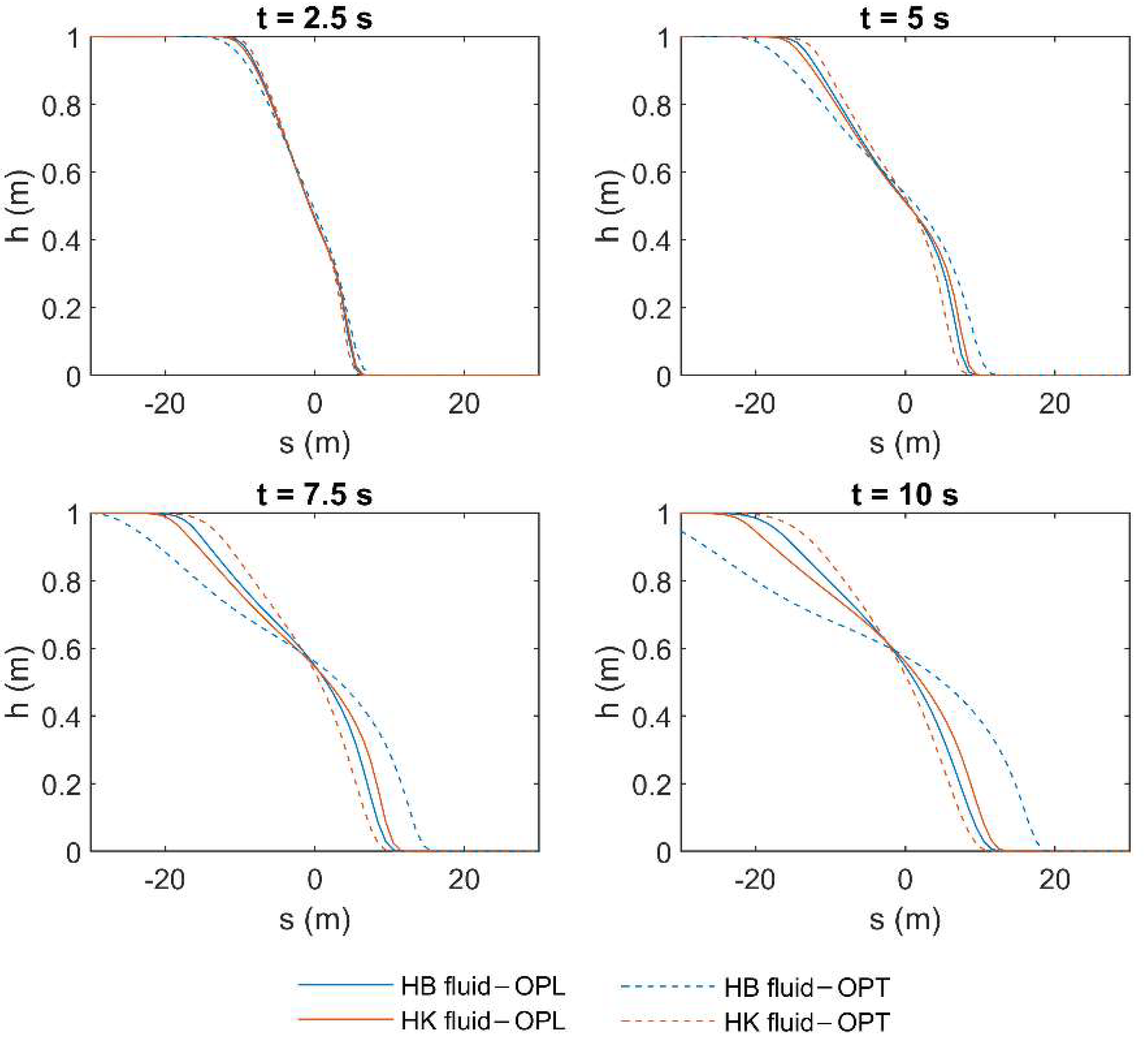
The results of the HLL in terms of fluid depth (
), obtained by using the constitutive parameters in both HB and HK for the highest tested concentration (i.e.,
= 0.25), are shown hereafter.
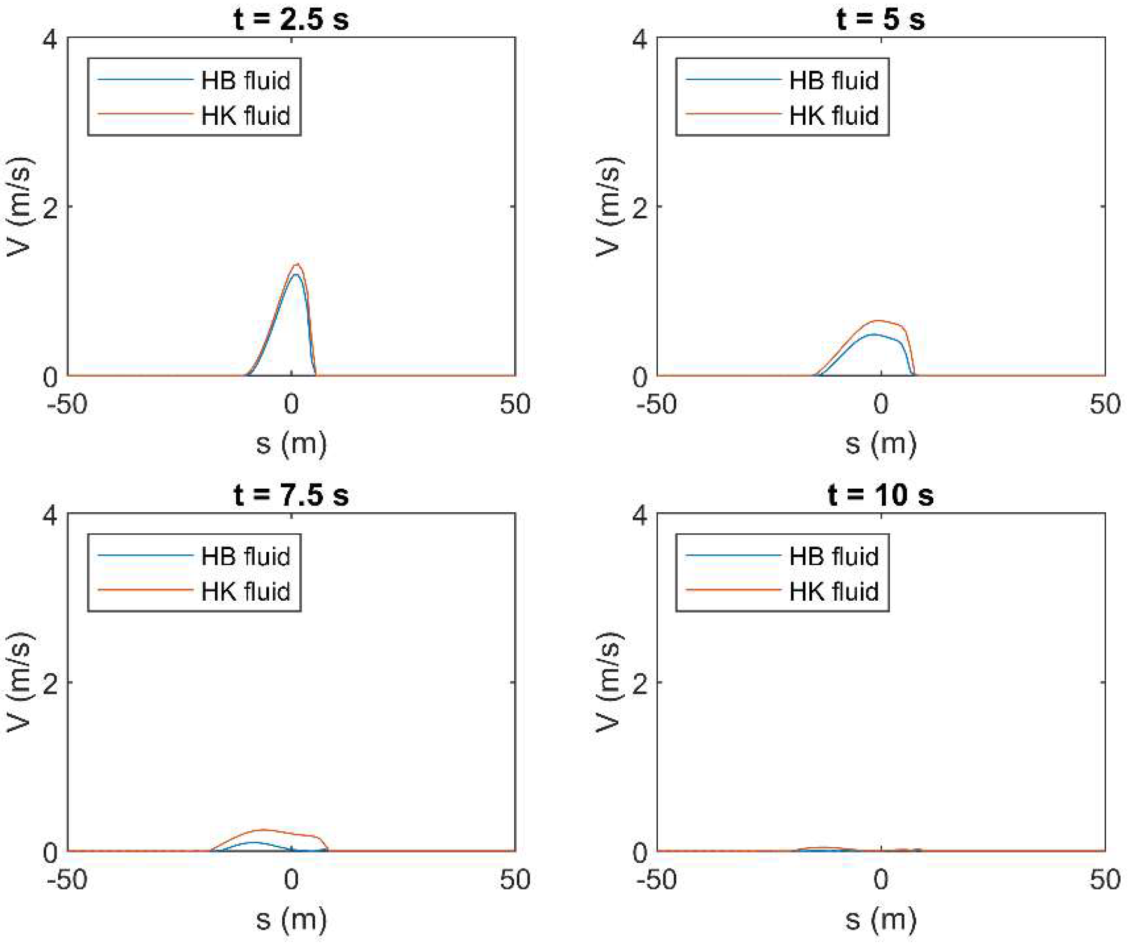
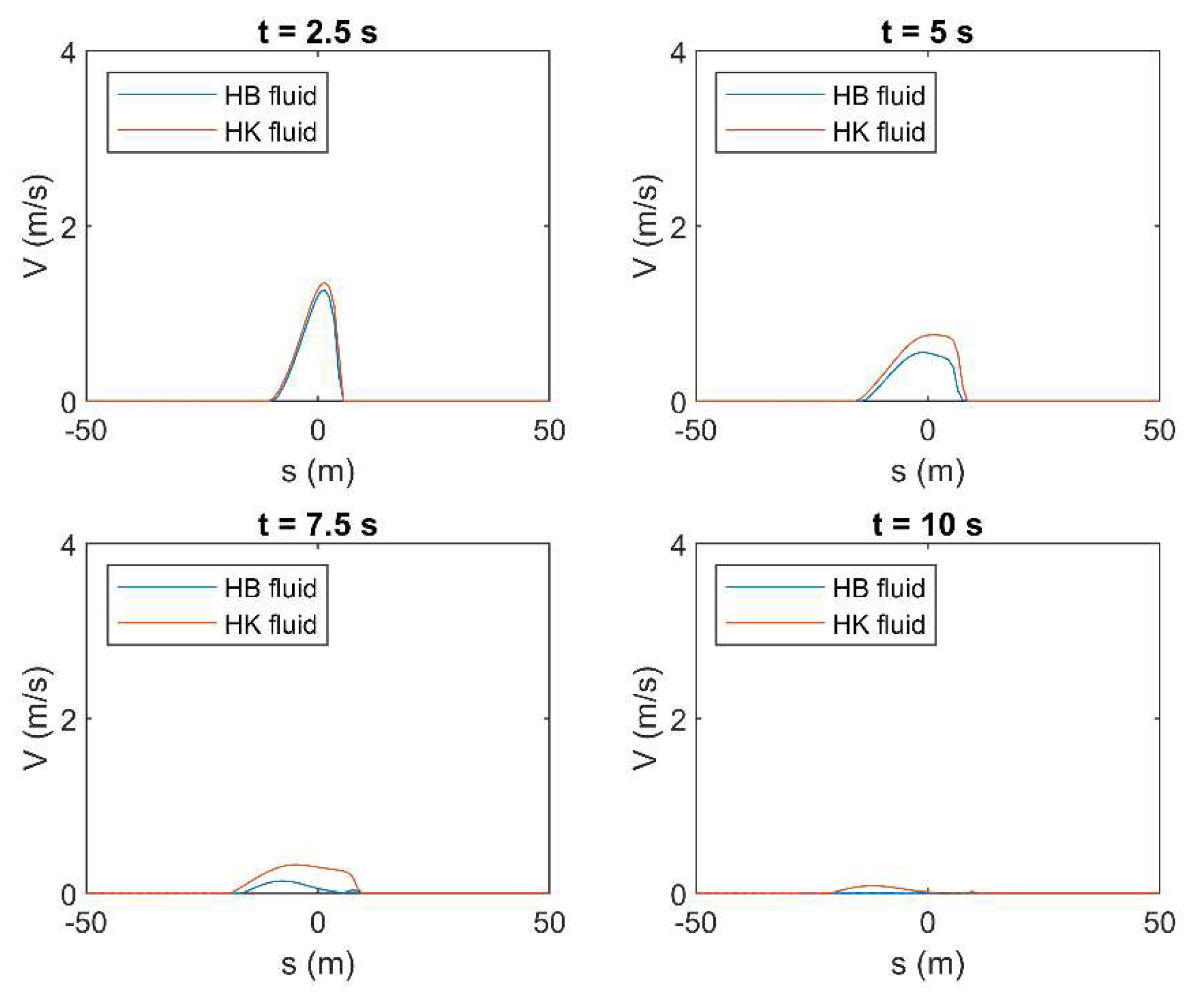
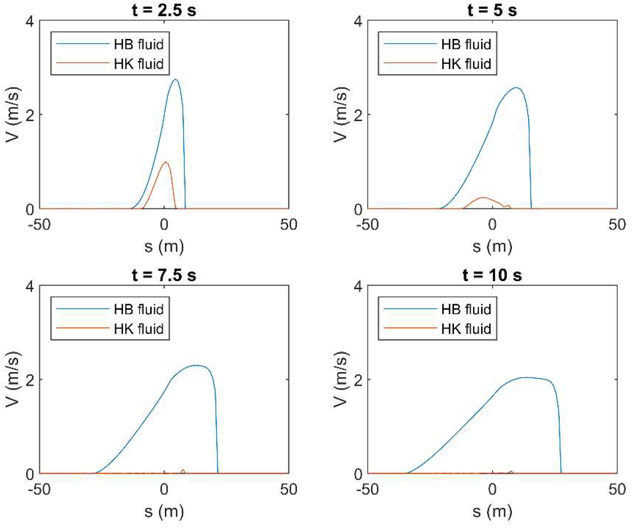
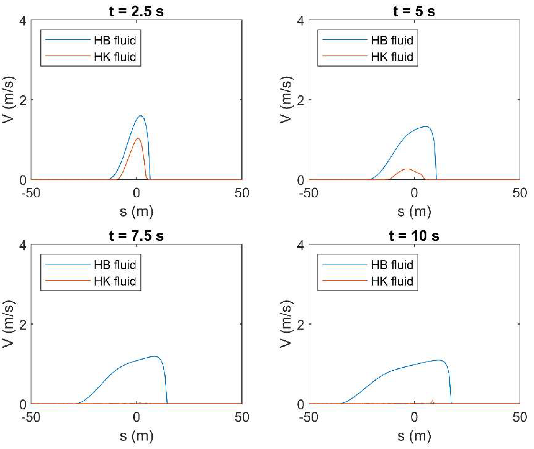
Figure 9 and
Figure 10 show the fluid profile resulting from the use of both OPL and OPT rheological parameters, for laminar and turbulent flow condition, respectively. These profiles are presented for different time instants between 0 and 10 s, with a step of 2.5 s. According to the results, if the fluid is modeled by the constitutive parameters obtained by fitting laminar data (i.e., OPL), the choice of the rheological model seems not to significantly affect the fluid behavior, and the resulting profiles approximately overlap, no matter if the flow regime is laminar or turbulent. Conversely, the profile resulting from OPT for the HB fluid is remarkably different from the other profiles. This is perfectly coherent with the results presented in the previous section, where the HK model resulted in exhibiting a better performance in terms of average errors, especially when the fluid is modeled according to the constitutive parameters obtained by fitting turbulent data (i.e., OPT). This behavior is highlighted for the highest concentration value. Moreover, as previously presented in
Table 4 and
Table 5, in laminar flow condition, such errors can be greater than in turbulent condition for high values of concentrations, and this results in the greater discrepancy between the depth profiles in
Figure 9. The same considerations are valid with reference to the mean velocity profiles, which are presented in
Appendix B. Moreover, with reference to the profiles resulting from OPT when HB is used as rheological model, the wave tip, that is, the part of the fluid front where the shear stresses are not negligible, is particularly evident. In the wave tip, such shear stresses are significant due to the high values of mean velocity (see
Appendix B). Conversely, in the other plots, the wave tip is not discernible since the shear stresses are remarkably high within the whole profile, as proven by the small values of velocity, which tend to zero at the last time instant (see
Appendix B).
The following tables (
Table 8,
Table 9,
Table 10,
Table 11,
Table 12 and
Table 13) show the results of the dam-break simulation in terms of average shear stress (
), maximum shear stress (
) and angle formed by the wave tip and the bottom line (δ), in laminar and turbulent flow condition, by using the rheological parameters obtained by OPL and OPT when both HB and HK are used as constitutive models. According to
Table 8,
Table 9,
Table 10 and
Table 11, the optimization on turbulent data (i.e., OPT) for the HB model results in values of
and
significantly smaller than all other results. This can be considered as a further evidence of the better performance of the HK model compared to the HB model, especially in OPT. The same consideration can be made with reference to the values of δ presented in
Table 12 and
Table 13.
7. Conclusions
The rheology of non-Newtonian fluids, i.e., the relation between the shear stress and the deformation velocity within a flow, is a crucial aspect in the fluid dynamic modeling, both in laminar and in turbulent conditions. Once the rheological model is chosen, the velocity profile can be integrated and uniform flow resistance formula can be also obtained. Then, several theoretical, semiempirical, or empirical models described the influence of the rheology in turbulent conditions.
The rheological analysis can be carried out either by means of rheometers based on a direct measurement of both the shear stress and the deformation velocity or by head loss measurements in uniform flow. The latter technique has been used for years in laminar conditions, based on the study of Rabinowitsch (1929) [
27] and Mooney (1931) [
28]. Recently, Carravetta et al. (2016) [
35] proposed a methodology to investigate the rheological behavior of a water sediment non-Newtonian mixture by performing experiments in turbulent uniform flow conditions. The possibility of using turbulent flow data can be crucial when the mixture has a large tendency for sedimentation, which can be an obstacle for testing the fluid in laminar conditions.
As a rheological model, the Herschel-Bulkley equation [
3] has been used for years to describe the non-Newtonian behavior of a large number of fluids and mixtures with yield stress. Nevertheless, this model presents some well-known inconsistencies at a high shear rate. Thus, Hallbom and Klein in 2009 [
8] presented a new rheological yield-stress model overcoming the Herschel-Bulkley [
3] inconsistencies.
In this study, the two rheological models are compared in terms of capacity of interpretation of both laminar and turbulent head loss in uniform flow conditions. A large set of experiments on a yield plastic fluid (i.e., a water–bentonite mixture) was available, and the parameter of Hershel-Bulkley [
3] and Hallbom and Klein [
8] models were fitted over the uniform flow data, in both laminar and turbulent conditions. The integration of the velocity profile was used to derive the resistance formulas in laminar flow, while the Thomas and Wilson model [
34] was used to predict the turbulent flow. Then, an optimization technique was applied to find the optimal values of the rheological parameters minimizing the difference between the measured and predicted mean velocity data. The results, in terms of errors in the prediction of the flow behavior, show that the Hallbom and Klein model [
8] outperforms the Herschel-Bulkley model [
3] to predict the turbulent flow when the laminar data are used to characterize the fluid, as well as to predict the laminar flow relying on turbulent data. Moreover, the variability of the Hallbom and Klein [
8] parameters with respect to the concentration is even smaller than the variability of the Herschel-Bulkley [
3] parameters, demonstrating a higher consistency of the more recently proposed rheological model.
Finally, a simple case study was considered, modeling the first instance of a dam-break phenomenon with the aim of highlighting the differences in terms of flow simulation arising from a different rheological modeling of the fluid. The results were presented, for both HB and HK rheological models, in terms of fluid depth, mean velocity, shear stress, and inclination of the wave tip, by using both the OPL and OPT parameters, in laminar and turbulent flow conditions. The high discrepancy between the results of OPT for the HB fluid and all other results further proves the well-known inconsistencies of the HB model compared to the HK model. The internal consistency of an HK model when rheological parameters are obtained by fitting turbulent data (i.e., OPT) allows one to perform reliable tests on sediment the mixtures, where experiments in laminar flow condition would be instead problematic, due to the sedimentation tendency.


