Article

Rayleigh–Bénard Instability of an Ellis Fluid Saturated Porous Channel with an Isoflux Boundary

by
Pedro Vayssière Brandão
,
Michele Celli
and
Antonio Barletta
*,†
Department of Industrial Engineering, Alma Mater Studiorum Università di Bologna, Viale Risorgimento 2, 40136 Bologna, Italy
*
Author to whom correspondence should be addressed.
These authors contributed equally to this work.
Fluids 2021, 6(12), 450; https://doi.org/10.3390/fluids6120450
Submission received: 13 November 2021 / Revised: 30 November 2021 / Accepted: 7 December 2021 / Published: 11 December 2021
(This article belongs to the Collection Non-Newtonian Fluid Mechanics)

Abstract

:
The onset of the thermal instability is investigated in a porous channel with plane parallel boundaries saturated by a non–Newtonian shear–thinning fluid and subject to a horizontal throughflow. The Ellis model is adopted to describe the fluid rheology. Both horizontal boundaries are assumed to be impermeable. A uniform heat flux is supplied through the lower boundary, while the upper boundary is kept at a uniform temperature. Such an asymmetric setup of the thermal boundary conditions is analysed via a numerical solution of the linear stability eigenvalue problem. The linear stability analysis is developed for three–dimensional normal modes of perturbation showing that the transverse modes are the most unstable. The destabilising effect of the non–Newtonian shear–thinning character of the fluid is also demonstrated as compared to the behaviour displayed, for the same flow configuration, by a Newtonian fluid.

1. Introduction

The emergence of convection Rayleigh–Bénard cells in a fluid saturated porous medium heated from below is a cornerstone topic in the research on convection heat transfer in porous solids. There is an impressively wide literature on this topic, often called Darcy–Bénard instability, which is surveyed in Chapter 6 of Nield and Bejan [1]. Other surveys relative to this area of research are provided by Straughan [2], Barletta [3]. Except for a minor part of the papers available in the literature regarding the Darcy–Bénard instability, most investigators have focussed their attention on the Newtonian fluids saturating a porous medium.
The Darcy–Bénard instability for saturating fluids with a non–Newtonian rheology has been investigated with reference to viscoelastic fluids [4,5,6], to fluids with yield–stress [7] and to purely viscous fluids [8,9,10,11,12,13,14]. In particular, Barletta and Nield [8], Alves and Barletta [9], Celli et al. [10] and Petrolo et al. [11] discuss the onset of the Darcy–Bénard instability in a porous medium by considering the power–law model. A more sophisticated model, i.e. Carreau–Yasuda, is employed by Brandão and Ouarzazi [12] and by Brandão et al. [13] to model purely viscous, non–Newtonian flow in porous media.
The usual setup envisaged in the studies on the onset of Darcy–Bénard instability in a saturated porous layer is one where the plane parallel boundaries are considered as isothermal with different temperatures. In the present paper, the objective is to extend the analysis carried out by Celli et al. [14]. In fact, Celli et al. [14] employ Ellis’ model to describe the behaviour of a shear–thinning non–Newtonian fluid saturating a porous medium. The temperature boundary conditions are modified, with respect to the study developed by Celli et al. [14], by assuming a uniform heat flux on the lower boundary of the layer. Such a modification is accompanied by a numerical solution of the stability eigenvalue problem, whereas an analytical dispersion relation is available with isothermal boundary conditions [14]. The shear–thinning rheology of the fluid is formulated by adopting the Ellis model extension of Darcy’s law. Results will be discussed for the instability onset in terms of the neutral stability curves and of the critical values of the perturbation wavenumber and of the Darcy–Rayleigh number. The main result is the demonstration of the destabilising effect of the Ellis fluid rheology as compared to the Newtonian fluid behaviour, with the transverse normal modes leading the transition to the instability.

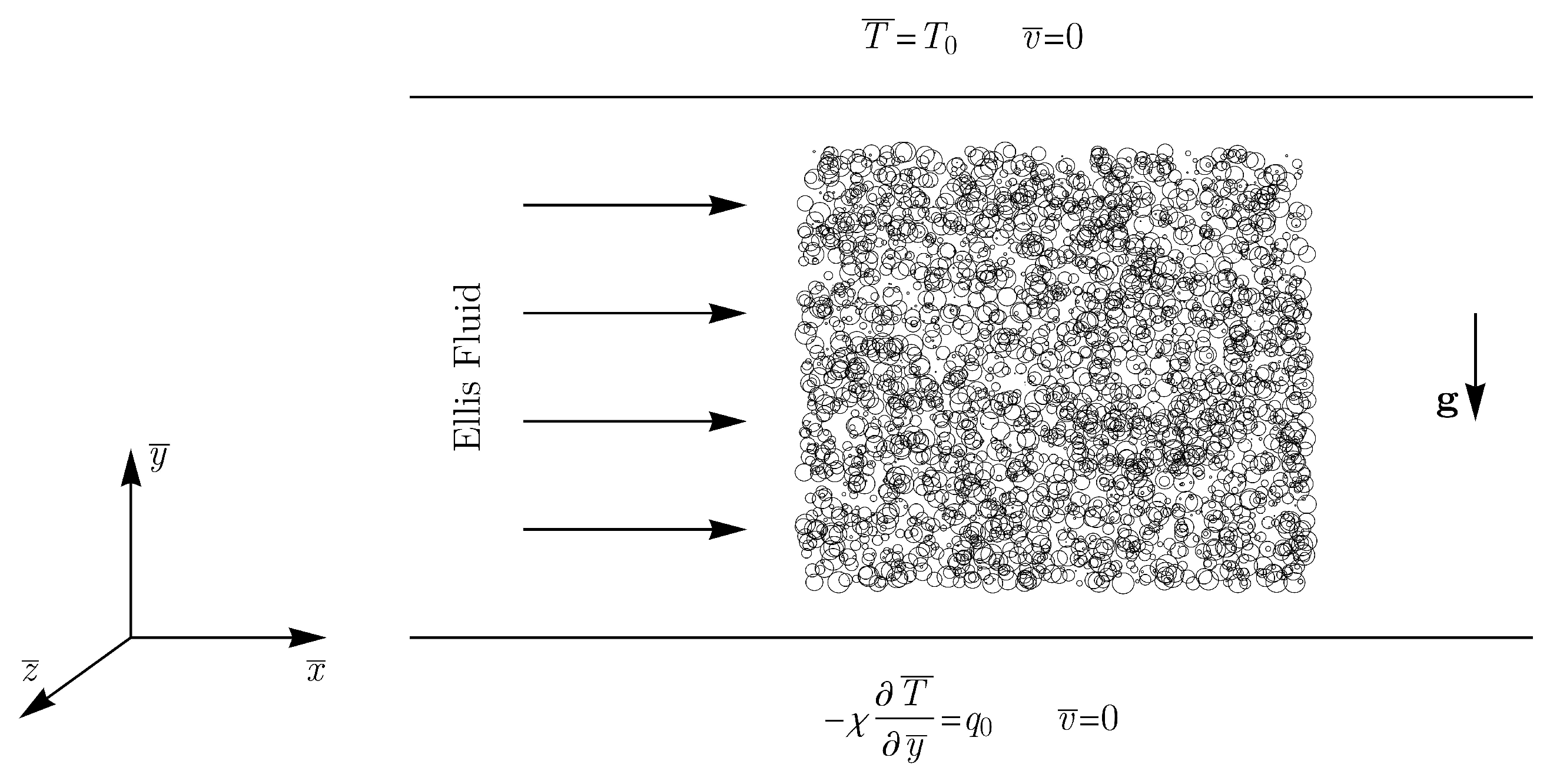
2. Mathematical Formulation

A porous layer of height H saturated by a non–Newtonian fluid is considered. The boundary walls are considered to be impermeable. The layer is heated from below by a constant heat–flux q 0 , while the upper boundary is kept at a constant temperature T 0 . A sketch of the porous layer with a scheme of the boundary conditions and of the coordinate axes is displayed in Figure 1. The Oberbeck–Boussinesq approximation is employed and local thermal equilibrium between the fluid and the solid matrix is assumed. A basic uniform throughflow is imposed along the horizontal x direction.

2.1. Rheological Model

The rheological behaviour of the non–Newtonian fluid is described by employing the Ellis model. More precisely, such a model is based on three–parameters that describe the rheology of a time–independent, shear–thinning and non–yield–stress fluid [15]. According to Sochi [15], the Ellis model is more reliable than the power–law model in matching the experimental data. The apparent viscosity η , according to the Ellis model, is given by [15,16].
η = η 0 1 + τ τ 1 / 2 ζ 1 ,
where ζ is a positive parameter such that ζ = 1 / n , where n is the power–law index. The apparent viscosity at zero shear–stress is represented by η 0 , while τ 1 / 2 represents the value of τ at which η = η 0 / 2 . By employing the power–law index, Equation (2) can be rewritten as
η = η 0 1 + τ τ 1 / 2 1 n n .
The apparent viscosity predicted by the Ellis model, for some limiting cases, is given by the following list:
τ 1 / 2 0 η = 0 , τ 1 / 2 η = η 0 , τ < τ 1 / 2 , n 0 η = η 0 , τ > τ 1 / 2 , n 0 η = 0 , n 1 η = η 0 / 2 .
On the other hand, in the limiting case of strong shear stresses, τ τ 1 / 2 , Equation (2) reduces to
η = η 0 τ τ 1 / 2 n 1 n .

2.2. Generalization of Darcy’s Law

For a Newtonian fluid saturating a porous medium, Darcy’s law can be formulated as [1]
u ¯ = K η f ¯ d ,
where the bars over the symbols represent the dimensional fields, time and coordinates. Here, u ¯ is the seepage velocity vector with components ( u ¯ , v ¯ , w ¯ ) , K is the permeability of the porous medium and f ¯ d is the drag force which contains the pressure gradient and the buoyancy term based on the Oberbeck–Boussinesq approximation, namely [1]
f ¯ d = p ¯ ρ 0 g β ( T ¯ T 0 ) .
In Equation (6), p ¯ is the local difference between the pressure and the hydrostatic pressure, ρ 0 is the fluid density evaluated at the reference temperature T 0 , g is the gravity acceleration vector and β is the thermal expansion coefficient of the fluid. Darcy’s law can be generalised for non–Newtonian fluids by replacing the fluid viscosity with an effective viscosity [16,17]. Hence, Equation (5) becomes
u ¯ = K η e f f f ¯ d ,
where η e f f is the effective viscosity given by
1 η e f f = 1 η 0 1 + 4 n 3 n + 1 | f ¯ d | r h τ 1 / 2 1 n n .
Here, r h is the mean hydraulic radius, which is directly proportional to the square root of the permeability of the porous medium divided by its porosity φ [16]
r h = 5 K φ .
Thus, the modified Darcy’s law for a porous medium saturated by an Ellis fluid can be rewritten in a more convenient way as
u ¯ = K η 0 1 + A | f ¯ d | 1 n n f ¯ d ,
where A is a coefficient determined by the properties of the porous medium and of the fluid,
A = 4 n 3 n + 1 r h τ 1 / 2 1 n n .
It is worth noting that, near the instability threshold, the drag forces have, usually, a small magnitude. In fact, in the limit of vanishing drag forces, f ¯ d 0 , Equation (10) reduces to Equation (5).

2.3. Governing Equations

The mass balance, momentum balance and energy balance equations for the present problem are given by
· u ¯ = 0 , η 0 K u ¯ = 1 + A | f ¯ d | 1 n n f ¯ d , f ¯ d = p ¯ ρ 0 g β ( T ¯ T 0 ) , σ T ¯ t ¯ + u ¯ · T ¯ = α 2 T ¯ , y ¯ = 0 : v ¯ = 0 , χ T ¯ y ¯ = q 0 , y ¯ = H : v ¯ = 0 , T ¯ = T 0 .
In Equation (12), σ is the ratio between the average volumetric heat capacity of the porous medium and the volumetric heat capacity of the fluid; α and χ are the average thermal diffusivity and the average thermal conductivity of the saturated porous medium, respectively.
The following scaling allows one to express Equation (12) in a dimensionless form
x = x ¯ H , u = H α u ¯ , p = K η 0 α p ¯ , t = α σ H 2 t ¯ , T = T ¯ T 0 Δ T ,
where Δ T = q 0 H / χ and x is the position vector with Cartesian components ( x , y , z ) . By substituting Equation (13) into Equation (12), one may write
· u = 0 , u = 1 + El | f d | 1 n n f d , T t + u · T = 2 T , y = 0 : v = 0 , T y = 1 , y = 1 : v = 0 , T = 0 ,
where
f d = p + R T e y .
The parameter El is the Darcy–Ellis number and the parameter R is the Darcy–Rayleigh number. They are defined as follows:
El = A α η 0 H K 1 n n , R = ρ g β H K Δ T α η 0 .

2.4. Basic State

The stationary solution of the problem is given by a uniform throughflow in the horizontal direction and by a negative vertical temperature gradient. The latter is due to the supplied heat flux on the bottom and the prescribed temperature on the top. The uniform throughflow is generated by a prescribed constant pressure drop along the x axis, p b / x . Thus, the basic solution is expressed as
u b = p b x 1 + El p b x 1 n n , v b = 0 , w b = 0 , p b y = R T b , p b z = 0 , T b = 1 y ,
where the subscript b denotes the basic state. Without any loss of generality, we can assume that p b / x is negative, so that u b assumes only positive values.

2.5. Linear Stability Analysis

In order to simplify the numerical treatment, the governing equations can be rewritten by employing a pressure–temperature formulation. By considering the first Equation (14) and by applying the divergence operator to the second Equation (14), we can get the rid of the velocity field in the momentum balance equation. For the energy balance equation, we employ the second Equation (14) to express the velocity as function of pressure. Thus, the pressure–temperature formulation of the governing equations is given by
· 1 + El | f d | 1 n n f d = 0 , T t + 1 + El | f d | 1 n n f d · T = 2 T , f d = p + R T e y , y = 0 : p y = R T , T y = 1 , y = 1 : p y = 0 , T = 0 ,
where the boundary conditions based on the pressure–temperature formulation are obtained by employing the governing Equation (14).

2.6. Normal Modes

The stability of the system is investigated by decomposing pressure and temperature into two parts: one relative to the basic equilibrium solution, and the other relative to the infinitesimal disturbances. The stability analysis consists in observing the linear evolution in time of such disturbances in order to determine the threshold values of the governing parameters for the onset of the instability. Such disturbances are investigated through a normal mode analysis. The decomposed pressure and temperature are given by
p ( x , y , z , t ) = p b ( x , y ) + ε f ( y ) e λ t e i k x x + k z z ω t , T ( x , y , z , t ) = T b ( y ) + ε h ( y ) e λ t e i k x x + k z z ω t ,
where λ is the growth rate, k x and k z are the wavenumbers in the x and z direction, ω is the angular frequency, f and h are the eigenfunctions of the problem, and ε is a positive parameter that defines the amplitude of the disturbances. Since ε 1 , all terms O ( ε 2 ) are neglected in the present analysis.
The instability threshold is determined by seeking the neutral stability, which is the transitional condition given by the normal modes with a zero growth rate. The present analysis is focussed on the dynamics of the most unstable normal modes arising in the system. By imposing λ = 0 , we ensure the neutral stability condition. Hence, the differential dispersion relation for the disturbances is given by
f ˜ n ˜ k 2 f ˜ R ˜ h = 0 , h ( k 2 R ˜ i ω ˜ ) h f ˜ = 0 ,
subject to the boundary conditions
y = 0 : f ˜ = R ˜ h , h = 0 , y = 1 : f ˜ = 0 , h = 0 ,
where the following quantities have been defined:
f ˜ = ( 1 + El ˜ ) f , R ˜ = ( 1 + El ˜ ) R , El ˜ = El p b x 1 n n , k x = k cos ϕ , k z = k sin ϕ , n ˜ = El ˜ + n ( El ˜ + 2 ) + El ˜ ( 1 n ) cos ( 2 ϕ ) 2 n ( El ˜ + 1 ) .
Here, ϕ is the angle between the wave vector of the normal mode and the x axis. In Appendix A, a proof that the eigenvalue problem is to be solved with ω ˜ = 0 is provided. In Appendix B, it is shown that the most unstable modes are the transverse rolls, whose wave vector is parallel to the basic flow direction ( ϕ = 0 ) . These findings are the basis for the discussion of the results presented in the forthcoming section.

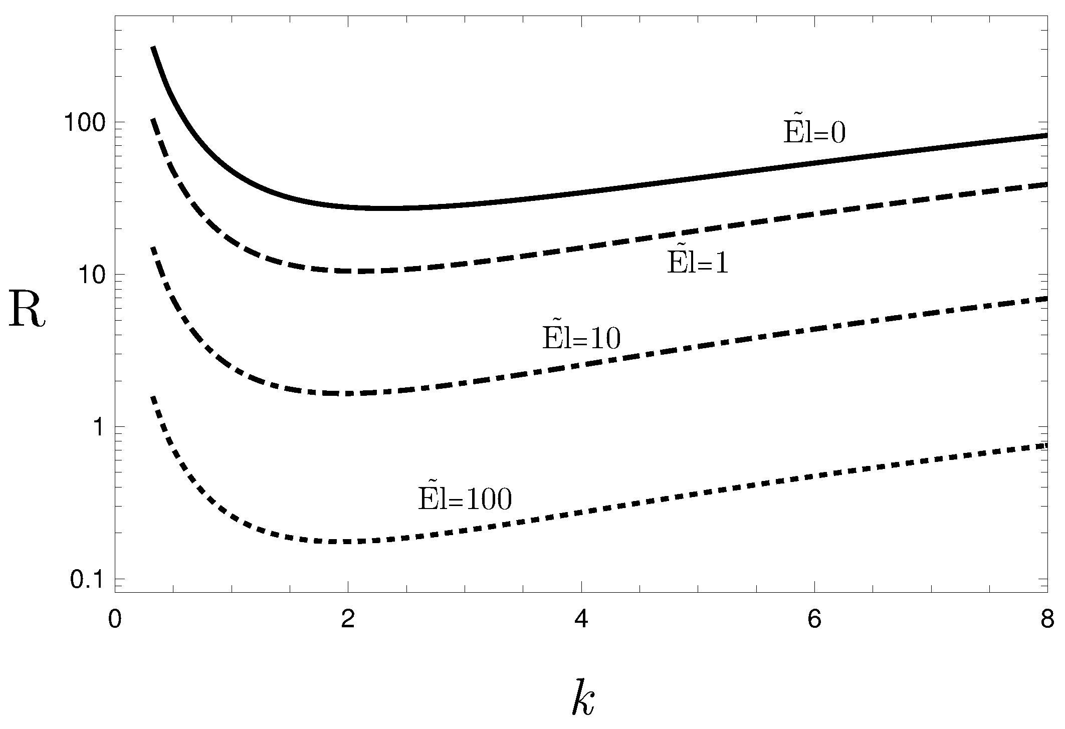
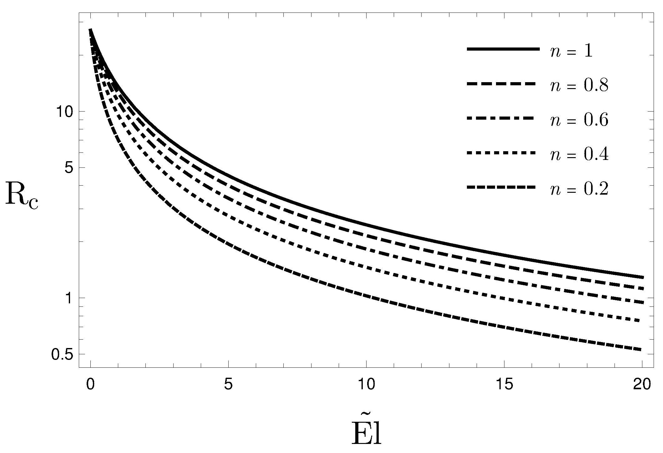
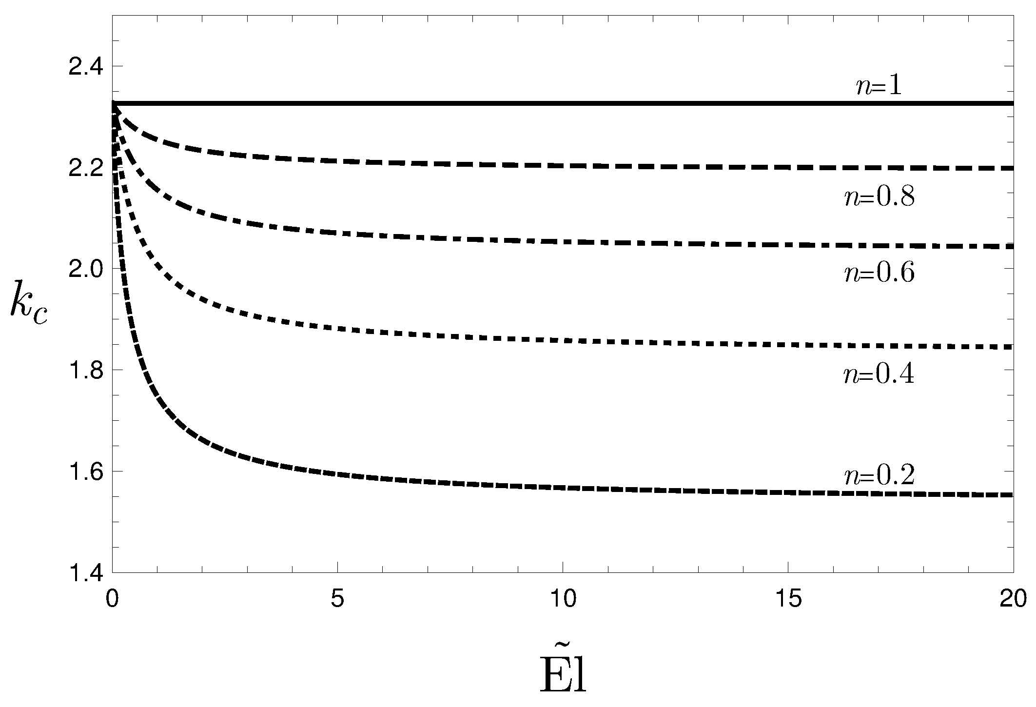
3. Results and Discussion

Equations (20) together with the boundary conditions (21) are solved numerically by using the procedure described in Appendix C. The results of the stability analysis are presented by displaying the neutral stability curves and the plots of the critical values of R and k versus the governing parameters ( El ˜ , n ).
In Figure 2, the neutral threshold is displayed in the ( k , R ) plane for different values of El ˜ and n = 0.5 . It is evident that the parameter El ˜ has a destabilising effect. In fact, with any fixed wavenumber k, the neutral stability condition for increasing values of El ˜ is achieved for decreasing values of R .
The most important information of a neutral stability curve is the global minimum of R , which defines the critical condition. In order to compute directly the critical points, one can derive the original Equation (20), as well as the boundary conditions (21), with respect to k and impose the condition R / k = 0 . The derivative of the eigenfunctions f ˜ and h with respect to k are treated as new eigenfunctions and the differential system expanded in this way is solved together with the original one. More information regarding this technique can be found in the paper by Alves et al. [18] and in the book by Barletta [3].
Figure 3 and Figure 4 show the critical stability condition by reporting R c and k c as functions of El ˜ for different values of n. By analysing these results, the destabilising role of El ˜ is confirmed. In addition, one may note that, for a vanishing El ˜ , the critical data do not depend on n. Indeed, a vanishing value of El ˜ means either El 0 or p b / x 0 . The first case means absence of a shear–thinning effect, as suggested by the second Equation (14), while the second case means no basic shear stress and, thus, no influence of the shear–thinning effect on the dynamics. In both cases, we expect that the Ellis fluid behaves as a Newtonian fluid. In fact, for El ˜ 0 , we obtain critical values that coincide with those reported in the literature for Newtonian fluids [1], namely R c = 27.1 and k c = 2.33 .
Figure 5 and Figure 6 show similar findings, even if R c and k c are presented as functions of n for different values of El ˜ . Again, the conclusion that, for El ˜ 0 , the critical data do not depend on n is confirmed. One may also note that, by increasing the value of El ˜ , the value of R c decreases with n. For a nonzero value of El ˜ , the critical value of R depends on n and this dependence becoming weaker and weaker as n 1 . Figure 6 shows that, for nonzero values of El ˜ , the critical wavenumber tends to k c = 2.33 when n 1 . In the limiting case n 0 , there is a significant decrease of both R c and k c .
Figure 7 displays the isolines of both pressure and temperature, showing the cellular flow pattern for El ˜ = 10 and n = 0.5 . The convective cells are evidently asymmetric with respect to the horizontal midplane. This is due to the different type of conditions imposed at the horizontal boundaries.

4. Conclusions

The linear convective instability of shear–thinning fluids saturating a porous channel has been investigated. The lower channel wall has been considered as subject to a uniform heat flux, while the upper wall is maintained at a constant temperature. The rheology of the shear–thinning fluid is described by employing the Ellis model. More precisely, a modified version of Darcy’s law has been assumed to represent the shear–thinning behaviour of the fluid. A study of small–amplitude disturbances has been proposed in order to determine the threshold for the onset of instability. The resulting system of differential equations, defining the stability eigenvalue problem, has been solved numerically. The governing parameters of this analysis are the modified Ellis number, El ˜ , the power–law index n, the Darcy–Rayleigh number R , the wavenumber k and the inclination angle ϕ of the wave vector to the basic flow direction. The main results can be summarized as follows:
  • The transverse rolls turned out to be the most unstable modes.
  • The neutral stability curves display, qualitatively, the same shape when changing the fluid flow parameters.
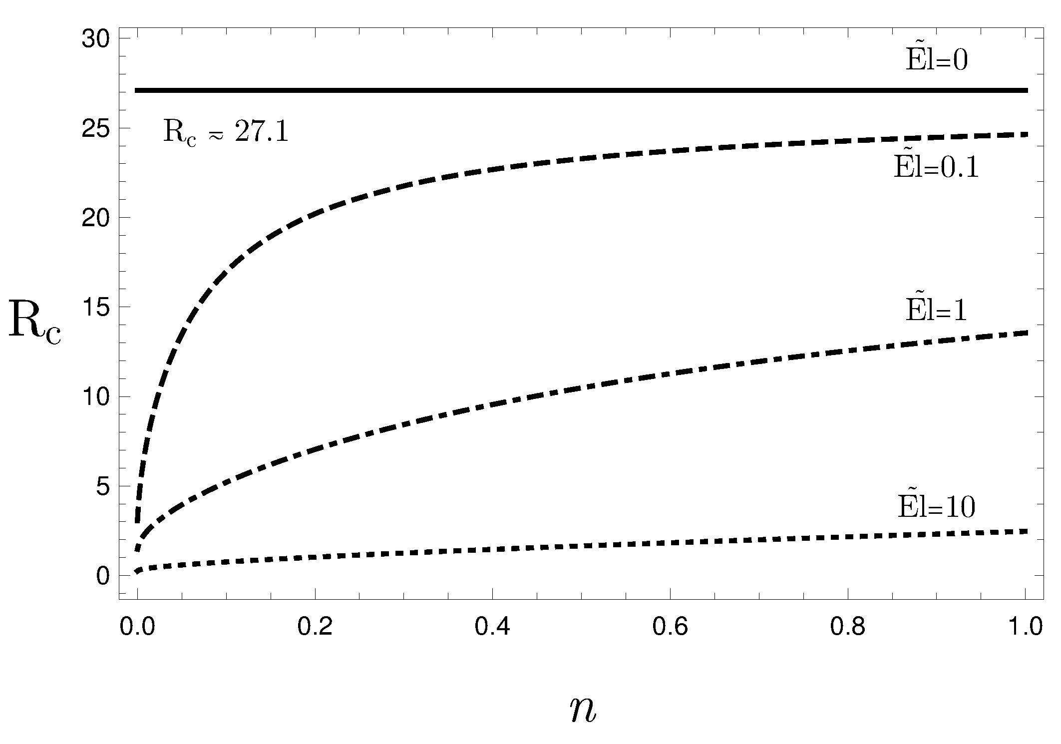
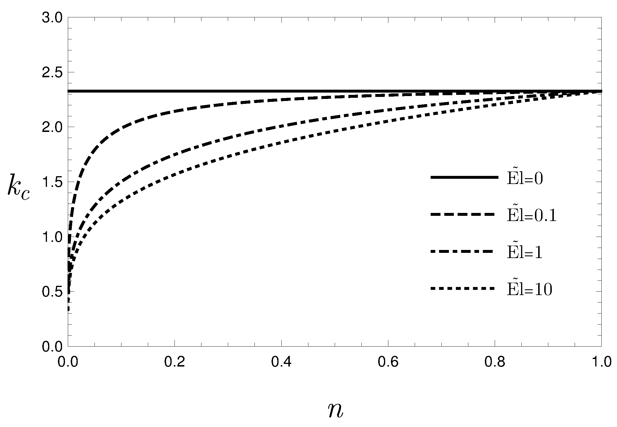
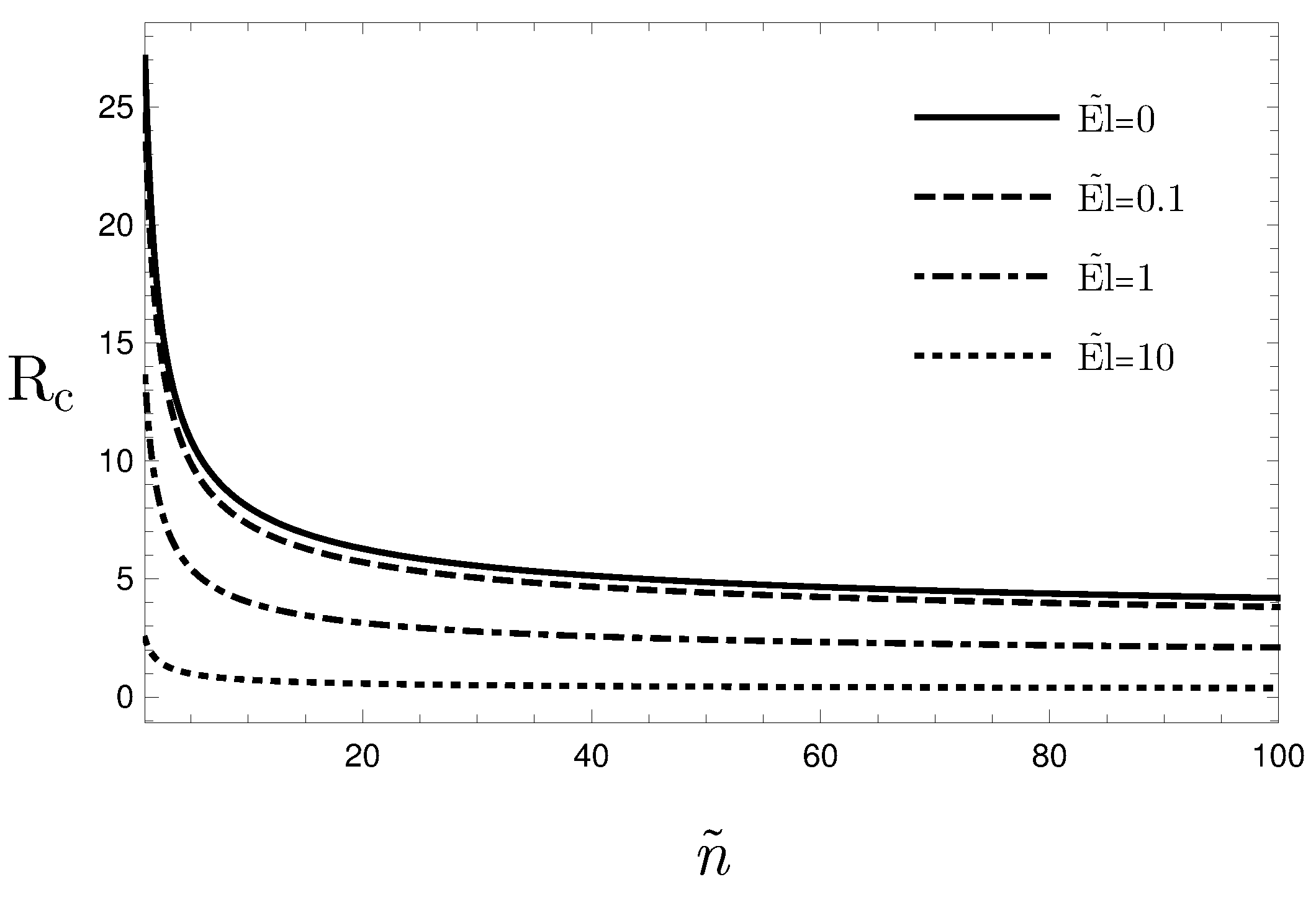
  • The effect of decreasing the value of n on the threshold value for the onset of the instability is similar to the effect of increasing the value of the modified Ellis number, El ˜ : both decreasing n or increasing El ˜ yield a destabilising effect.
  • When El ˜ 0 , the onset of the instability is not affected by n and the critical values of the governing parameter match the values reported in the literature for Newtonian fluids, namely R c = 27.1 and k c = 2.33 .

Author Contributions

Conceptualization P.V.B., M.C. and A.B.; methodology P.V.B., M.C. and A.B.; validation P.V.B., M.C. and A.B.; formal analysis P.V.B., M.C. and A.B.; investigation P.V.B., M.C. and A.B.; writing–original draft preparation P.V.B., M.C. and A.B.; writing–review and editing P.V.B., M.C. and A.B.; funding acquisition P.V.B., M.C. and A.B. All authors have read and agreed to the published version of the manuscript.

Funding

This study was financed in part by the Coordenação de Aperfeiçoamento de Pessoal de Nível Superior–Brazil (CAPES)–Grant n 88881.174085/2018–01. Financial support was also provided by Ministero dell’Istruzione, dell’Università e della Ricerca (Italy)–Grant n PRIN2017F7KZWS.

Conflicts of Interest

The authors declare no conflict of interest. The funders had no role in the design of the study; in the collection, analyses, or interpretation of data; in the writing of the manuscript, or in the decision to publish the results.

Appendix A. A Proof That ω ˜ = 0

In order to prove that ω ˜ = 0 , we multiply the first Equation (20) by the complex conjugate of the eigenfunction f ˜ , f ˜ * . Then, after integrating by parts and using the boundary conditions given by Equation (21), one obtains
0 1 | f ˜ | 2 d y + k 2 n ˜ 0 1 | f ˜ | 2 d y R ˜ 0 1 h f ˜ * d y = 0 .
From Equation (A1), by recognising that the first two terms are both real and positive, we reach the conclusion that
0 1 h f ˜ * d y R ,
where R denotes the set of real numbers. By taking the complex conjugate of the integral in Equation (A2), we conclude also that
0 1 f ˜ h * d y R .
We multiply the second Equation (20) by the complex conjugate of h, h * , and we integrate by parts over the domain y ( 0 , 1 ) to obtain
0 1 | h | 2 d y + k 2 R ˜ i ω ˜ 0 1 | h | 2 d y + 0 1 f ˜ h * d y = 0 .
By utilising Equation (A3), we may now split Equation (A4) into its real and imaginary parts to get
ω ˜ 0 1 | h | 2 d y = 0 .
Finally, by recalling that the trivial solution ( h = 0 ) must be excluded, we conclude that
ω ˜ = 0 .

Appendix B. Dominant Modes

If we account for the dependence of n ˜ on ϕ , we can say that n ˜ is a monotonic decreasing function of ϕ , considering that 0 ϕ π / 2 . The proof is simple: we evaluate d n ˜ / d ϕ from Equation (22),
d n ˜ d ϕ = El ˜ ( 1 n ) sin ( 2 ϕ ) n ( El ˜ + 1 ) .
Since n 1 and sin ( 2 ϕ ) 0 within the interval 0 ϕ π / 2 , one can easily conclude that d n ˜ / d ϕ 0 , i.e., that n ˜ is a monotonic decreasing function of ϕ .
Thus, by looking at Figure A1, we can observe that R c is a monotonic decreasing function of n ˜ . Hence, we can infer that R c is a monotonic increasing function of ϕ . This conclusion implies that the most unstable modes are transverse ( ϕ = 0 ) .
Figure A1. Critical value of R as a function of n ˜ for different values of El ˜ .
Fluids 06 00450 g0a1

Appendix C. Numerical Method

The numerical method used to solve the differential eigenvalue problem is the shooting method. The basis of this method is the reformulation of the original eigenvalue problem (20), subject to the boundary conditions (21), as an initial value problem by using additional initial conditions, namely
f ˜ n ˜ k 2 f ˜ R ˜ h = 0 , h k 2 R ˜ h f ˜ = 0 , f ˜ ( 0 ) = R ˜ h ( 0 ) , f ˜ ( 0 ) = 1 , h ( 0 ) = 0 , h ( 0 ) = ξ .
We mention that the initial condition f ˜ ( 0 ) = 1 can be imposed because the governing differential equations in (A8) are homogeneous. On the other hand, ξ is an unknown real parameter to be found. The system of Equation (A8) is solved numerically by means of the Runge–Kutta method. The solution for the eigenfunctions f ˜ and h depends on the four governing parameters, k, n ˜ , R ˜ and ξ . Such parameters are to be determined through a root–finding algorithm in order to satisfy the target conditions
f ˜ ( 1 ) = 0 , h ( 1 ) = 0 .
A comparison between our results and those reported in Chapter 6 of the book by Nield and Bejan [1] reveals, in the special case El 0 , an excellent agreement, with k c = 2.33 and R c = 27.1 .

References

  1. Nield, D.A.; Bejan, A. Convection in Porous Media, 5th ed.; Springer: New York, NY, USA, 2017. [Google Scholar]
  2. Straughan, B. Stability and Wave Motion in Porous Media; Springer: New York, NY, USA, 2008. [Google Scholar]
  3. Barletta, A. Routes to Absolute Instability in Porous Media; Springer: New York, NY, USA, 2019. [Google Scholar]
  4. Kim, M.C.; Lee, S.B.; Kim, S.; Chung, B.J. Thermal instability of viscoelastic fluids in porous media. Int. J. Heat Mass Transf. 2003, 46, 5065–5072. [Google Scholar] [CrossRef]
  5. Hirata, S.C.; Ouarzazi, M.N. Three–dimensional absolute and convective instabilities in mixed convection of a viscoelastic fluid through a porous medium. Phys. Lett. A 2010, 374, 2661–2666. [Google Scholar] [CrossRef]
  6. Pallavi, G.; Hemanthkumar, C.; Shivakumara, I.S.; Rushikumar, B. Oscillatory Darcy–Bénard–Poiseuille mixed convection in an Oldroyd–B fluid–saturated porous layer. In Advances in Fluid Dynamics; Springer: New York, NY, USA, 2021; pp. 827–837. [Google Scholar]
  7. Rees, D.A.S. Darcy–Bénard–Bingham convection. Phys. Fluids 2020, 32, 084107. [Google Scholar] [CrossRef]
  8. Barletta, A.; Nield, D. Linear instability of the horizontal throughflow in a plane porous layer saturated by a power–law fluid. Phys. Fluids 2011, 23, 013102. [Google Scholar] [CrossRef]
  9. Alves, L.S.d.B.; Barletta, A. Convective instability of the Darcy–Bénard problem with through flow in a porous layer saturated by a power–law fluid. Int. J. Heat Mass Transf. 2013, 62, 495–506. [Google Scholar] [CrossRef]
  10. Celli, M.; Barletta, A.; Longo, S.; Chiapponi, L.; Ciriello, V.; Di Federico, V.; Valiani, A. Thermal instability of a power–law fluid flowing in a horizontal porous layer with an open boundary: A two–dimensional analysis. Transp. Porous Media 2017, 118, 1–23. [Google Scholar] [CrossRef]
  11. Petrolo, D.; Chiapponi, L.; Longo, S.; Celli, M.; Barletta, A.; Di Federico, V. Onset of Darcy–Bénard convection under throughflow of a shear–thinning fluid. J. Fluid Mech. 2020, 889, R2. [Google Scholar] [CrossRef]
  12. Brandão, P.V.; Ouarzazi, M.N. Darcy–Carreau model and nonlinear natural convection for pseudoplastic and dilatant fluids in porous media. Transp. Porous Media 2021, 136, 521–539. [Google Scholar] [CrossRef]
  13. Brandão, P.V.; Ouarzazi, M.N.; Hirata, S.C.; Barletta, A. Darcy–Carreau–Yasuda rheological model and onset of inelastic non–Newtonian mixed convection in porous media. Phys. Fluids 2021, 33, 044111. [Google Scholar] [CrossRef]
  14. Celli, M.; Barletta, A.; Brandão, P.V. Rayleigh–Bénard instability of an Ellis fluid saturating a porous medium. Transp. Porous Media 2021, 138, 679–692. [Google Scholar] [CrossRef]
  15. Sochi, T. Non–Newtonian flow in porous media. Polymer 2010, 51, 5007–5023. [Google Scholar] [CrossRef] [Green Version]
  16. Sadowski, T.J.; Bird, R.B. Non–Newtonian flow through porous Media. I. Theoretical. Trans. Soc. Rheol. 1965, 9, 243–250. [Google Scholar] [CrossRef]
  17. Sadowski, T.J. Non–Newtonian flow through porous media. II. Experimental. Trans. Soc. Rheol. 1965, 9, 251–271. [Google Scholar] [CrossRef]
  18. Alves, L.D.B.; Hirata, S.D.C.; Schuabb, M.; Barletta, A. Identifying linear absolute instabilities from differential eigenvalue problems using sensitivity analysis. J. Fluid Mech. 2019, 870, 941–969. [Google Scholar] [CrossRef]
Figure 1. A sketch of the porous layer, of the boundary conditions and of the coordinate axes.
Fluids 06 00450 g001
Figure 2. Neutral stability curves for n = 0.5 and different values of El ˜ .
Fluids 06 00450 g002
Figure 3. Critical value of R as a function of El ˜ for different values of n.
Fluids 06 00450 g003
Figure 4. Critical wavenumber k c as a function of El ˜ for different values of n.
Fluids 06 00450 g004
Figure 5. Critical value of R as a function of n for different values of El ˜ .
Fluids 06 00450 g005
Figure 6. Critical wavenumber k as a function of n ˜ .
Fluids 06 00450 g006
Figure 7. Isolines of pressure (left) and temperature (right) drawn for El ˜ = 10 and n ˜ = 0.5 .
Fluids 06 00450 g007
Publisher’s Note: MDPI stays neutral with regard to jurisdictional claims in published maps and institutional affiliations.

