Flow Structures Identification through Proper Orthogonal Decomposition: The Flow around Two Distinct Cylinders

Abstract

Numerical simulations of fluid flows can produce a huge amount of data and inadvertently important flow structures can be ignored, if a thorough analysis is not performed. The identification of these flow structures, mainly in transient situations, is a complex task, since such structures change in time and can move along the domain. With the decomposition of the entire data set into smaller sets, important structures present in the main flow and structures with periodic behaviour, like vortices, can be identified. Therefore, through the analysis of the frequency of each of these components and using a smaller number of components, we show that the Proper Orthogonal Decomposition can be used not only to reduce the amount of significant data, but also to obtain a better and global understanding of the flow (through the analysis of specific modes). In this work, the von Kármán vortex street is decomposed into a generator base and analysed through the Proper Orthogonal Decomposition for the 2D flow around a cylinder and the 2D flow around two cylinders with different radii. We consider a Newtonian fluid and two non-Newtonian power-law fluids, with $n=0.7$ and $n=1.3$. Grouping specific modes, a reconstruction is made, allowing the identification of complex structures that otherwise would be impossible to identify using simple post-processing of the fluid flow.

1. Introduction

The Proper Orthogonal Decomposition (POD) method was first introduced by Lumley in 1967 [1], and it allows for decomposing almost any flow into an infinite set of eigenfunctions or modes. The objective of the POD method is to reduce the model in a way that it can capture the most important and reliable information with much less data and effort. This method is famous in Computational Fluid Dynamics (CFD) because it reduces the simulation time and allows for predicting the fluid flow based only on the most important modes.

Since 1967, several versions of the POD method (and even new methods) were proposed in the literature, being adapted to specific cases and branches of engineering (it should be remarked that, in the first fifteen years, the only works on this topic are from Lumley itself, some co-workers, and Ph.D. students [2]).

The method has become very popular and has been applied to a wide variety of engineering problems going from fluid mechanics to bio-engineering, having different names for the same procedure: Karhunen–Loève Decomposition, Principal Components Analysis (PCA), Singular Systems Analysis, and Singular Value Decomposition (SVD) (please see the review papers [3,4]). To name all the works on the POD method [5] would be a tedious task that is out of the scope of this work, although some of these works are worth mentioning.

Regarding POD, Selin Aradag et al. [6] developed a couple of methods (the Hybrid Filtered POD (HFPOD) approach (see also [7]) and the Fast Fourier Transform (FFT)-based 3D Filtered POD (FFTPOD)) to deal with the difficulty encountered when using simple POD for three-dimensional (3D) structures. Using the HFPOD method, large-scale structures associated with von Kármán’s vortex street, as well as their phase and amplitude variations, can be identified quantitatively. FFTPOD enables modeling 3D flows without being contaminated by small-scale turbulent structures while capturing the large-scale features of the flow, like von Kármán’s vortex street. The filtering steps (in the HFPOD method) must be repeated until most small-scale structures are qualitatively eliminated. A spanning phase is provided by the HFPOD, but the FFTPOD is able to deal with 3D geometry, making it a promising alternative to the Hybrid POD for 3D flows.

For a space-time POD problem, for statistically stationary flows, Aaron et al. [8] investigated the Spectral Proper Orthogonal Decomposition (SPOD). This model produces modes that oscillate at a single frequency. In their study, the authors demonstrated how SPOD modes articulate coherently with development in space and time, in contrast to general POD space-modes. Moreover, SPOD modes were found to be optimally averaged Dynamic Mode Decompositions (DMD), resulting from an ensemble model DMD problem for stationary flows. In this sense, SPOD modes represent dynamic structures in the same sense as DMD modes while also incorporating the statistical variability of turbulent flows.

It should be mentioned that the POD method is not the only technique used in the literature to predict complex fluid flows with less effort. We have, for example, Machine Learning (ML) that is now a hot topic on this subject. In fact, the POD method is a feature selection method used in Data Mining processes, to reduce the dimension of the process [9] (in this area, the POD method goes by the name of PCA). Thus, combining the CFD simulations and ML algorithms to simultaneously reduce computational cost and time, retain physical insight by focusing on the prediction of flow-fields, and keep the ability to access information or to make adjustments is already a reality [10].

The flow around one cylinder is well understood and documented in the literature. See, for example, [11]. Regarding more recent literature on the use of POD to study the flow around bluff bodies, we have the works by Bergmann et al. [12] where they studied the optimal rotary control of the cylinder wake using POD. Huan Ping et al. [13] also studied the wake dynamics behind a rotary oscillating cylinder. They used POD to extract the energetic modes that govern the dynamics of the flow, and also to characterize the spatially evolving nature of the forced wake as it undergoes a transition from the near-wake two-layer shedding pattern to the far-wake Kármán-like shedding pattern. The authors concluded that only a few modes allowed for reconstructing the near-wake accurately, while more modes must be retained to ensure an accurate approximation of the far-wake. Riches et al. [14] used POD to analyze the wake-dynamics of a low-mass ratio circular cylinder undergoing vortex-induced vibrations. Most of the more recent works are now flow around cylinders with different surface texture/geometry.

For the flow around two cylinders, we have works on flows around side-by-side circular cylinders with the same dimensions [15,16,17], and a study with two cylinders in a staggered configuration where the data processed by the POD method were obtained from experimental measurements of flow fields using the Particle Image Velocimetry (PIV) method [18]. Works on the flow around side-by-side circular cylinders of different radii seems to be nonexistent.

In this work, a simple POD method is used to compute the 2D flow around a single cylinder, and, around two cylinders of different radii. The novelty of this work is:

• the use of POD not to reduce (and compile) the amount of information on the flow (has happens in most studies), but to rather show that the POD can be used to capture flow structures and flow physics that would be impossible to observe without a mode analysis. Highlighting, in this way, this ability of the POD method;
• to further understand the flow around two cylinders of different radii, through the use of POD and classical CFD. By decomposing this complex 2D flow, we have a better comprehension of the impact that a certain obstacle has in areas of interest.

We present a detailed study on complex 2D flows, and it is shown that the energy drop-off for higher order modes is much less steep when the complexity of the 2D flow increases.

It should be mentioned that we do not consider turbulent flows. The idea is to fully understand the mode decomposition in an oscillatory flow around two parallel cylinders of different dimensions.

This work is organized as follows: first, we present the basics of POD. Then, numerical simulations for the 2D flow past a cylinder are performed, considering a Newtonian fluid and two non-Newtonian power-law fluids with $n=0.7$ and $n=1.3$. The most important modes are identified for this well known case. Then, we perform a numerical study on the 2D flow past two cylinders of different radii (for both Newtonian and power-law fluids). This specific flow destroys the possibility of forming a symmetric pattern over time and increases the difficulty in grouping different modes. We discuss in detail the dynamics of the fluid flow and the reconstruction procedure. The document ends with the conclusions.

2. Equations and Numerical Method

The equations governing the flow of an isothermal incompressible fluid are the continuity:

$$\nabla ·\mathbf{u}=0,$$

(1)

and the momentum equations,

$$\rho \frac{\mathrm{D}\mathbf{u}}{\mathrm{D}t}=-\nabla p+\nabla ·\tau ,$$

(2)

where $\frac{\mathrm{D}}{\mathrm{D}t}$ is the material derivative, p is the pressure and $\rho$ the fluid density, together with the constitutive equation $\tau =2\mu \mathbf{D}$, where $\mathbf{D}$ is the rate of deformation tensor and $\mu$ is the viscosity. For a Newtonian fluid, $\mu$ is constant.

2.1. Non-Newtonian Power-Law Fluid

For a non-Newtonian power-law fluid, the constitutive equation for $\mathit{\tau }$ is now given by:

$$\mathit{\tau }=\eta \left(\dot{\gamma }\right)\mathbf{D}$$

(3)

where $\eta \left(\dot{\gamma }\right)$ is the viscosity function, given by:

$$\eta \left(\dot{\gamma }\right)=K{\dot{\gamma }}^{n-1}$$

(4)

with K being the consistency index, n the power-law index, and $\dot{\gamma }$ the second invariant of the rate of deformation tensor (for simple shear flows, $\dot{\gamma }$ is just the shear rate).

For the study with the power-law fluid, the generalized Reynolds number is given by [19,20],

$$R{e}_{gen}=\frac{6\rho U^{\left(2-n\right)}{D}^n}{K{\left[\left(4n+2\right)/n\right]}^n},$$

(5)

where U is the imposed mean velocity at the inlet. When $n=1$, the model reduces to the classical Reynolds number $Re$,

$$Re=\frac{\rho UD}{\mu },$$

(6)

with $\eta \left(\dot{\gamma }\right)=K=\mu$ a constant viscosity.

2.2. Von Kármán Vortex Street

A von Kármán Vortex street is a repeating pattern of swirling vortices. This happens due to vortex shedding, which is responsible for the unsteady separation of flow of a fluid around a blunt body. When studying this phenomenon, an important dimensionless number is the Strouhal number (named after the Czech physicist, Vincenc Strouhal (1850–1922)). This dimensionless number is a key parameter for oscillating flows because it describes the relation between the length-scale of the blunt body, the vortex shedding frequency and the flow velocity [10]. The Strouhal number is defined by

$$St=\frac{fD}{U},$$

(7)

where f is the vortex shedding frequency and D is the diameter of the blunt body. This dimensionless number can be related to $Re$. According to Roshko [21], for approximately $50<Re<150$, the relationship between $St$ and $Re$ is given by

$$St=0.212\left(1-\frac{21.2}{Re}\right).$$

(8)

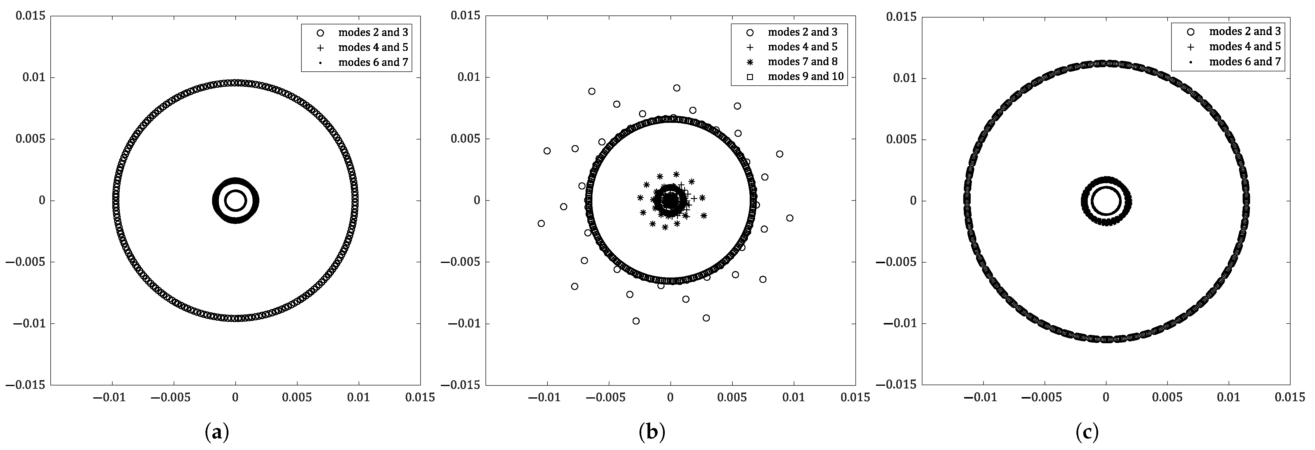
2.3. Proper Orthogonal Decomposition

To implement the POD method, we assumed that all data are saved in a matrix with a ${\left({\varphi }_1,{\varphi }_2,...,{\varphi }_{N_e}\right)}^T$ shape, saving one time step in each column. Thus, we obtained a matrix $\mathsf{\Phi }$ with $N_e$ by $N_t$ elements:

$$\mathsf{\Phi }=\left[\begin{array}{cccc}{\varphi }_{1,1}& {\varphi }_{1,2}& \cdots & {\varphi }_{1,N_t}\\ {\varphi }_{2,1}& {\varphi }_{2,2}& \cdots & {\varphi }_{2,N_t}\\ ⋮& ⋮& \ddots & ⋮\\ {\varphi }_{N_e,1}& {\varphi }_{N_e,2}& \cdots & {\varphi }_{N_e,N_t}\end{array}\right]$$

(9)

where $N_e$ is the number of elements to study and $N_t$ are the time steps.

For the study proposed in this work, the data saved in matrix $\mathsf{\Phi }$ corresponds to the velocity components, u and v, and the pressure, p, obtained after performing a CFD simulation. Thus, in each column of matrix $\mathsf{\Phi }$, ${\left(u_1,u_2,...,u_{N_E},v_1,v_2,...,v_{N_E},p_1,p_2,...,p_{N_E}\right)}^T$ are saved, where $N_E$ is the number of elements of the mesh. We can also consider other properties, such as temperature or viscosity.

Each column of $\mathsf{\Phi }$ can be written as a linear combination of orthonormal vectors or modes, $\mathbf{u}$. These modes are unitary and orthogonal. Therefore, the matrix of the modes, $\mathbf{U}$, is given by

$$\mathbf{U}=\left[\begin{array}{cccc}{u}_{1,1}& u_{1,2}& \cdots & u_{1,N_m}\\ u_{2,1}& u_{2,2}& \cdots & u_{2,N_m}\\ ⋮& ⋮& \ddots & ⋮\\ u_{N_e,1}& u_{N_e,2}& \cdots & u_{N_e,N_m}\end{array}\right]$$

(10)

where $N_m$ is the number of modes. This way, each element of matrix $\mathsf{\Phi }$ can be written as:

$${\displaystyle {\varphi }_{i,t}=\sum _{m=1}^{N_m}{u}_{i,m}{a}_{m,t}}$$

(11)

where $i\in \{1,2,\cdots ,N_e\}$, $t\in \{1,2,\cdots ,N_t\}$ and $a_{m,t}$ are the temporal coefficients.

Equation (11) in the matrix form becomes:

$$\mathsf{\Phi }=\mathbf{U}·\mathbf{A}.$$

(12)

where $\mathbf{A}$ is the matrix of the temporal coefficients and is equal to

$$\mathbf{A}=\left[\begin{array}{cccc}{a}_{1,1}& a_{1,2}& \cdots & a_{1,N_t}\\ ⋮& ⋮& \ddots & ⋮\\ a_{N_m,1}& a_{N_m,2}& \cdots & a_{N_m,N_t}\end{array}\right]$$

(13)

Matrices $\mathbf{U}$ and $\mathbf{A}$ are obtained by the autocovariance matrix $\mathbf{R}$ that is given by

$$\mathbf{R}=\frac{1}{N_e}\mathsf{\Phi }·{\mathsf{\Phi }}^T$$

(14)

whose eigenvectors are the columns of matrix $\mathbf{U}$. Matrix $\mathbf{A}$ is obtained by:

$$\mathbf{A}={\mathbf{U}}^T·\mathsf{\Phi }.$$

(15)

The distribution of the matrix $\mathbf{U}$ columns is directly related to the corresponding eigenvalues. This way, the first columns of $\mathbf{U}$ are the ones showing a higher variation of the temporal coefficients, and therefore the ones that gather more relevant information. Thus, we reconstruct matrix $\mathsf{\Phi }$, where only the modes that are more relevant are considered. Since $N_m<N_e$, it brings:

$$\mathsf{\Phi }\approx \tilde{\mathbf{U}}·\tilde{\mathbf{A}}=\tilde{\mathsf{\Phi }}$$

(16)

where $\tilde{\mathbf{U}}$ is the matrix with the first more relevant modes and $\tilde{\mathbf{A}}$ is the matrix with the temporal coefficients that correspond to the first more relevant modes, and $\tilde{\mathsf{\Phi }}$ is the spatial reconstruction of the properties in study. For more information on this subject, please consult [22,23,24] for a detailed explanation on the POD method implemented in this work.

2.4. Numerical Method

The system of equations (Equations (1) and (2)) were solved numerically using the software ANSYS Fluent version 2020 R2.

To perform the simulations, the velocity and pressure fields at $t=0$ were obtained in the following manner:

• First, a steady-state solution was calculated for $Re=100$;
• Second, the previous solution was used as an initial guess ($t=0$) for the velocity and pressure fields, in the steady-state turbulent numerical simulation considering $Re=500$. This simulation allowed the development of the characteristic von Kármán vortex street.
• Third, the steady-state solution obtained for $Re=500$ was used as the initial guess for our transient simulations with $Re=100$.

The pressure–velocity coupling was done using the SIMPLE method. To discretize the pressure gradient, the Least Squares Cell Based scheme was used, and, for the discretization of the advective terms, the Second-Order Upwind scheme was considered. The transient term was approximated by a first order implicit scheme. The POD analysis was performed with MATLAB R2018a.

In the next section, more details are presented regarding the geometry and meshes used along the work.

3. Case Study: Flow around a Single Cylinder

In this section, we present some results on the flow around a single cylinder that will be used fully in the analysis of the flow around two cylinders (for comparison).

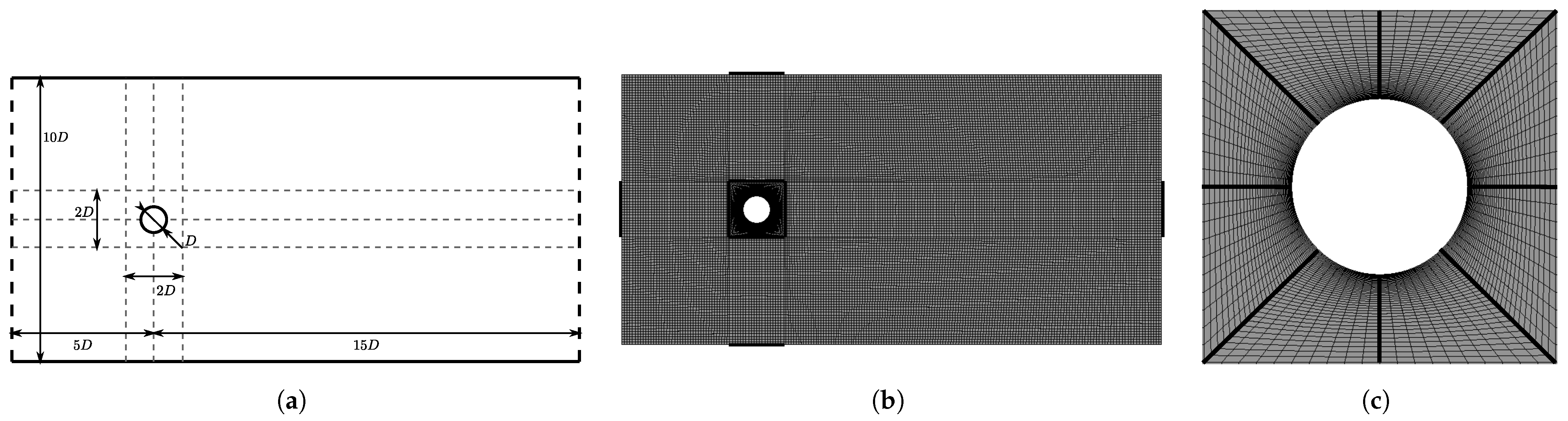
3.1. Geometry, Boundary Conditions, and Mesh

Figure 1a shows the geometry of the flow around a cylinder. The left bold-dashed line represents the inlet and the right dashed one the outlet. The cylinder has a diameter $D=0.1$ m and is placed $5D$ away from the inlet and $15D$ from the outlet. The inlet has a height $10D$. Regarding boundary conditions, we have imposed pressure at the outlet, and imposed at the inlet a uniform velocity profile that is constant in time. At the top and bottom walls of the channel, we consider full slip, and at the wall of the cylinder the usual empirical no-slip boundary condition was assumed.

To study the flow around one cylinder, we first perform a mesh study. We consider three meshes: one with $\mathrm{12,976}$ elements, one with $\mathrm{23,789}$ elements, and a more refined one with $\mathrm{48,570}$ elements. For each mesh, a simulation with 1000 time-steps was performed, and the drag coefficient on the cylinder wall was calculated. Then, we determined the average drag coefficient, $\overline{c_d}$, for each mesh. The results are presented in

Table 1. Average drag coefficient values for the three meshes.

Mesh	Number of Elements	$\overline{{\mathit{c}}_{\mathit{d}}}$
$M_1$	$\mathrm{48,570}$	$1.463$
$M_2$	$\mathrm{23,789}$	$1.470$
$M_3$	$\mathrm{12,976}$	$1.475$

.

We calculated an extrapolated value for $\overline{c_d}$ using the Richardson extrapolation technique,

$$\overline{c_{d_E}}\approx \overline{c_{d_{M_1}}}+\frac{\overline{c_{d_{M_1}}}-\overline{c_{d_{M_2}}}}{r^l-1},$$

(17)

where $\overline{c_{d_E}}$ is the extrapolated value, $\overline{c_{d_{M_1}}}$ is $\overline{c_d}$ for mesh $M_1$, $\overline{c_{d_{M_2}}}$ is the $\overline{c_d}$ for mesh $M_2$ and $\overline{c_{d_{M_3}}}$ is the $\overline{c_d}$ for mesh $M_3$. r is the grid refinement ratio and l is the order of the method. We see that $r\approx 2$, and, in this work, we assumed that $l=2$. Using Equation (17), we obtained $\overline{c_{d_E}}\approx 1.477$.

We measured the relative error (Equation (18)) for each mesh and obtained a good trade-off between accuracy and computational cost for mesh $M_2$. The error $\epsilon$ was small (about $0.42\%$):

$$\epsilon =\frac{|\overline{c_{d_E}}-\overline{c_{d_{M_2}}}|}{|\overline{c_{d_E}}|}=0.42\%.$$

(18)

Based on these results, the subsequent numerical simulations will be performed on mesh $M_2$.

Figure 1b shows a global view of the chosen mesh $M_2$ and Figure 1c shows a zoomed view of the mesh around the cylinder. The cell size was set to $0.0025$ m along the cylinder surface region, $0.01$ m along bold lines of Figure 1b and $0.02$ m on the rest of the domain. The cell size growth rate was $1.2$, and, along the edges in bold (Figure 1c), a bias type procedure was used with a bias factor of 10.

3.2. Rheological Properties

To perform the numerical simulations, we first considered a Newtonian fluid with the rheological properties of water at a temperature of 20 °C, that is, density $\rho ={10}^3$$\mathrm{kg}·{\mathrm{m}}^{-3}$, and viscosity $\mu ={10}^{-3}$$\mathrm{Pa}·\mathrm{s}$. We considered a Reynolds number of 100, which for a cylinder with diameter $D=0.1$ m, leads to an imposed inlet velocity U of ${10}^{-3}$$\mathrm{m}·{\mathrm{s}}^{-1}$. Then, we performed the numerical simulations with a non-Newtonian power-law fluid, where $R{e}_{gen}=100$, $\rho ={10}^3$$\mathrm{kg}·{\mathrm{m}}^{-3}$, $D=0.1$ m and $U={10}^{-3}$$\mathrm{m}·{\mathrm{s}}^{-1}$ is the imposed inlet velocity. We will consider two fixed values for the power-law index n: $0.7$ and $1.3$. Thus, from Equation (5), we conclude that $K=0.00039$ $\mathrm{Pa}·{\mathrm{s}}^{0.7}$ and $0.0026$ $\mathrm{Pa}·{\mathrm{s}}^{1.3}$, respectively.

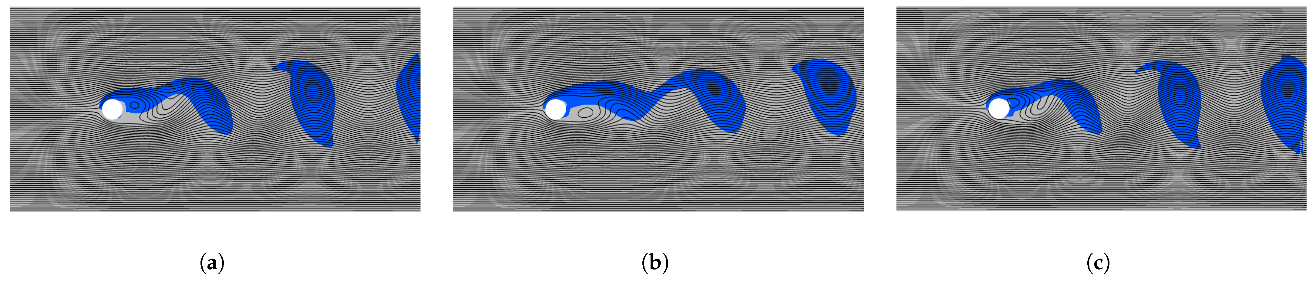
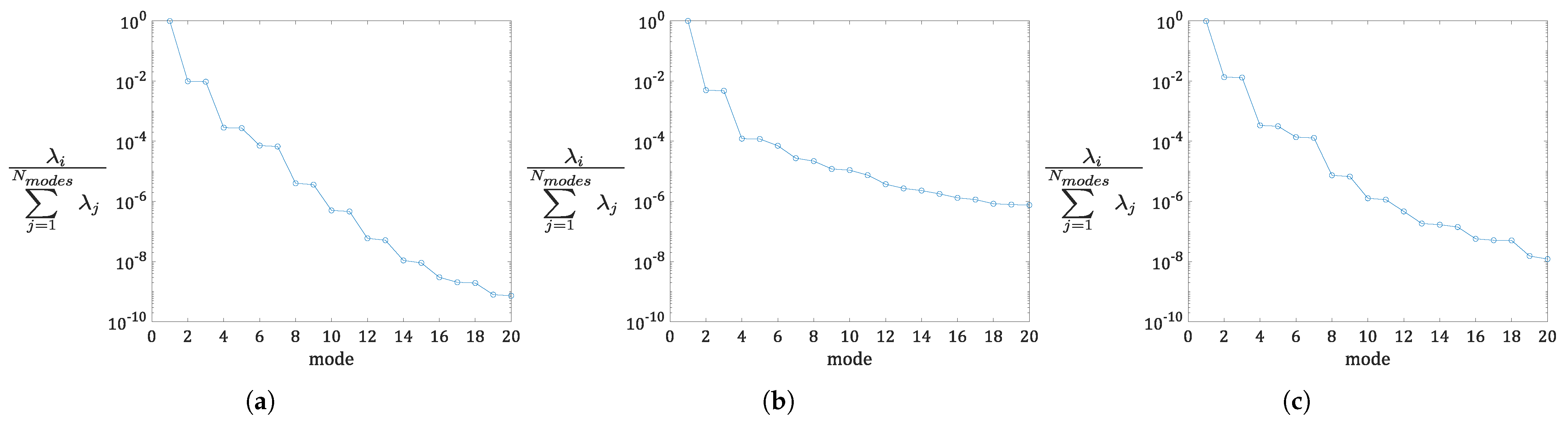
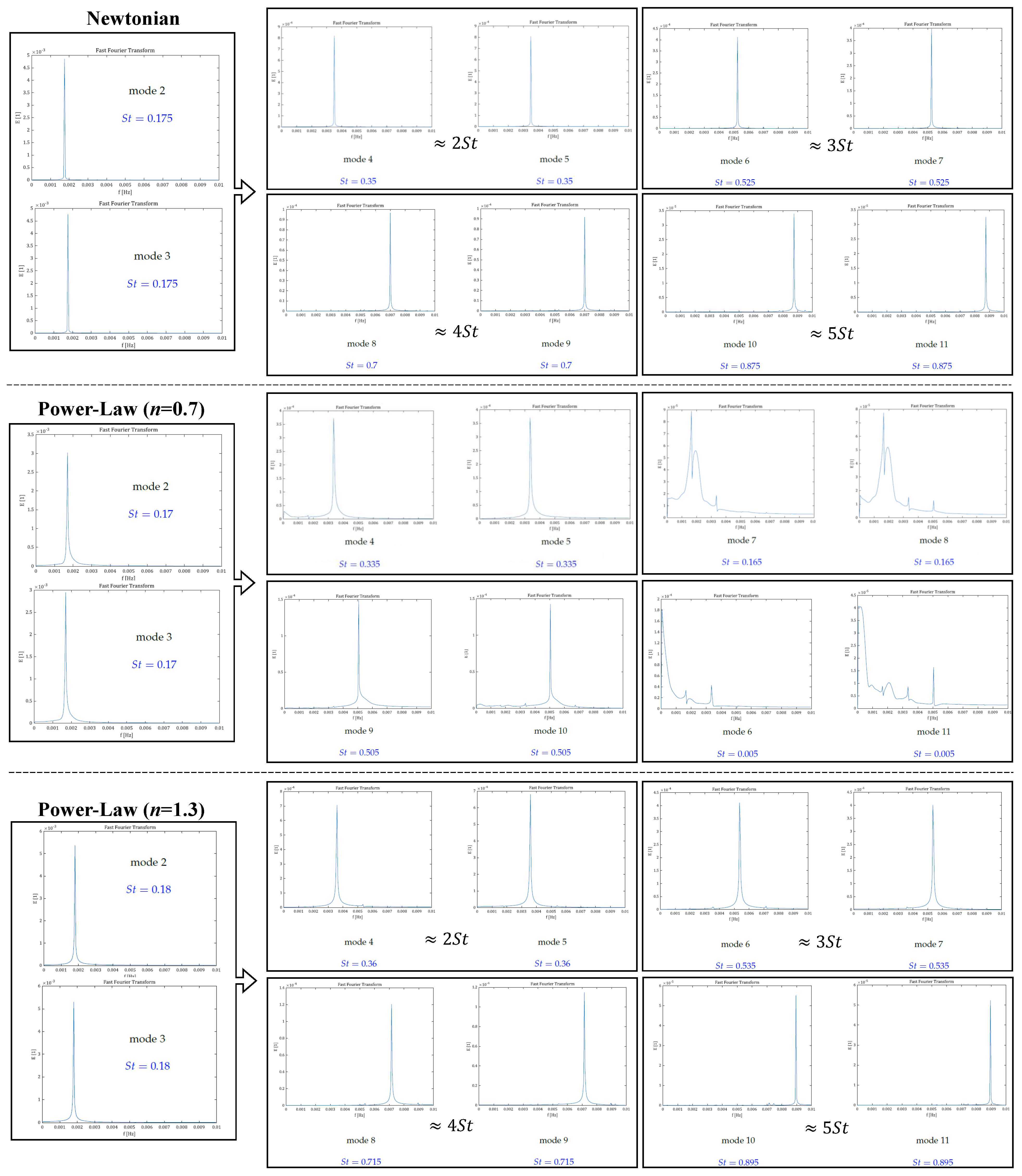
3.3. Results and Discussion

The transient simulation with $Re=100$ was performed and the first $10\lambda$ seconds $\left(\lambda =\frac{20D\times 10D}{10D\times u}\mathrm{s}\right)$ were ignored to avoid the strong influence of the initial conditions. Note that $\lambda$ is an approximate measure of the residence time, that is, the time a particle takes to go from the inlet to the outlet. The study and analysis was focused on the subsequent $10\lambda$ seconds of data.

To set the maximum time step of the numerical simulation, a maximum Courant number (C) of 1 was considered. A $C\le 1$ leads to $\delta t_{CFD}\le \frac{\delta x}{u_{max}}=\frac{0.0025}{0.001}=2.5$ s. To use the POD method, we considered the data of every 20 time-steps, i.e., $\delta t_{POD}=50$ s, resulting into 400 time-steps to be analyzed.

Figure 2a–c show the streamlines and the vorticity sign map at $t=20\lambda$, for a Newtonian fluid, and non-Newtonian power-law fluids with $n=0.7$ and $n=1.3$, respectively.

In Figure 2a, we see that vortices detach from the cylinder rear with diameter of about $5D$, and, from Equation (8), for $Re=100$, we have $St\approx 0.17\approx 1/5.88$. Therefore, the structures behind the cylinder are about six times bigger than the cylinder, or three times bigger with an alternating sign of rotation. The oscillatory behaviour downstream from the cylinder is perceptible, and the vortices on Figure 2c have a similar behaviour to the ones presented in Figure 2a for the Newtonian fluid.

In this work, due to the high computational effort and the existence of low information on the neglected modes, only the first 20 eigenvalues and modes were calculated.

Figure 3a–c show the relative weight of the eigenvalues associated with each modes, for the three fluids described before. For all cases, we see a fast decrease of the relative weight of the eigenvalues associated with each mode. In Figure 3a, the weights attributed to the first, second, and third eigenvalues are $98\%$, $0.98\%$, and $0.95\%$, respectively. In Figure 3b, the weights are $99\%$, $0.5\%$, and $0.47\%$, respectively. Finally, in Figure 3c, the weights are $97.2\%$, $1.3\%$, and $1.3\%$. All figures show residual weights attributed to the remaining modes, leading to the conclusion that only three modes allow the reconstruction of the flow.

Table 2. Most important modes (1 to 7) of u, v and p for the flow around a single cylinder. For each component u, v and p, we have from left to right: a Newtonian fluid, a power-law fluid with $n=0.7$ and a power-law fluid with $n=1.3$.

	u			v			p
1
2
3
4
5
6
7

presents the most important modes of u, v, and p (for each component u, v and p, we have from left to right: a Newtonian fluid, a power-law fluid with $n=0.7$, and a power-law fluid with $n=1.3$.).

Analysing the modes in Table 2, we see that the first mode is symmetric and has the main features of the flow without the oscillating components. For the Newtonian fluid and the power-law fluid with $n=1.3$, the modes after mode 1 are similar by pairs, with some delay between them. We also see that modes 2 and 3 are coherent with vortices. These vortices are about six times larger than the cylinder, as shown in Figure 2. For the power-law fluid with $n=0.7$, the modes after mode 1 are similar by pairs to modes 2 and 3 and modes 4 and 5, also with some delay between them, but mode 6 for u and p seems to be symmetrical again. Note that, from Figure 3b, after mode 5, the modes do not pair, having residual contributions. Therefore, it will be more difficult to analyse their contribution. We would probably need more simulation time or a smaller time-step to make a better analysis. We can see that, for the power-law fluid with $n=1.3$, the results are similar to the Newtonian case, and this may be explained by the dilatant, or shear-thickening behaviour (increase in apparent viscosity at higher shear rates). The flow is more sensible to the shear-thinning obtained for $n=0.7$, and therefore we have differences and similarities with the Newtonian results for $n=0.7$ and $n=1.3$, respectively.

Table 3. Comparison between the original (first row of images) data versus the partial reconstruction at $t=20\lambda$ seconds (the modes used in the reconstruction are shown in the first column). For each component u, v and p, we have from left to right: a Newtonian fluid, a power-law fluid with $n=0.7$ and a power-law fluid with $n=1.3$.

	u			v			p
2, 3
4, 5
1–3
1–5

shows a comparison between the original data obtained from the simulation and the partial reconstruction at $t=20\lambda$ (for each component u, v and p, we have from left to right: a Newtonian fluid, a power-law fluid with $n=0.7$, and a power-law fluid with $n=1.3$).

The reconstruction is made with modes 2 and 3, modes 4 and 5, modes 1 to 3 and modes 1 to 5. We see that the reconstruction with modes 2 and 3 allows us to recover the vortices traveling along the domain. With the reconstruction of the first three modes, almost all the structures are perceptible, although slight corrections to their shapes are needed. Comparing the reconstruction with modes 2 and 3, with the reconstruction with modes 4 and 5, we see that they are similar, but with smaller structures on the case of modes 4 and 5. These modes are a first correction to the above referred vortices. When we perform the reconstruction with the first five modes, the velocity and pressure maps become very similar to the original data.

Figure 4 shows an analysis of frequencies of the modes time coefficients for the three fluids. The Strouhal numbers (Equation (7)) presented in Figure 4 are calculated considering the frequency with higher energy, D as defined in Section 3.1 and U as defined in Section 3.2. By Equation (8), the Strouhal number with $Re=100$ is about $0.17$.

Analysing the Strouhal numbers in Figure 4 for the Newtonian fluid (top), we obtain $St=0.175$ that is similar to the one obtained from Equation (8). We can also see that the pair of modes 2 and 3, 4 and 5, 6 and 7, 8 and 9, 10 and 11, have common Strouhal number. This characteristic reveals that each pair is associated with the same flow structure. Furthermore, we notice that higher values of the Strouhal number are multiples of the Strouhal number of modes 2 and 3, so they can be considered as harmonic frequencies, as for example in the square wave function case. These harmonic frequencies result from the non-perfectly round shape of the vortices that travel along the domain.

When we analyse Figure 4 for the power-law fluid where $n=0.7$, we see that the pairs of modes that now have common Strouhal number are modes 2 and 3, modes 4 and 5, modes 7 and 8, modes 9 and 10 and, finally, modes 6 and 11. Now, modes 7 and 8 have a Strouhal number similar to Strouhal number of modes 2 and 3, the Strouhal number of modes 4 and 5 is about twice the Strouhal number of modes 2 and 3 and the Strouhal number of modes 9 and 10 is about the three times Strouhal number of modes 2 and 3. These mixed results come from the use of another constitutive model for viscosity. The results for a power-law fluid with $n=1.3$ are similar to the Newtonian ones, with only small differences.

The modes are unitary vectors whose weighted average (the linear combination) forms the original data set. Those weights are the time components and can be used to represent the importance of each mode. According to Figure 4, we can group the modes by consecutive pairs because of the similar Strouhal number. Therefore, in Figure 5, are represented the pairs of time coefficients for consecutive modes, for the three fluids. We can see that, from the contribution of modes 2 and 3, and 4 and 5, the oscillatory and alternating behaviour is perceived.

4. Case Study: Flow around Two Distinct Cylinders

We now consider two distinct cylinders that will cause the loss of symmetry and allow us to present the main contribution of this work. We perform a detailed analysis of this flow dynamics, and show that even in these complex cases we can perform a reconstruction of the flow using the basics of the POD method, and therefore obtain a reduction in data analysis and observe hidden structures in the flow.

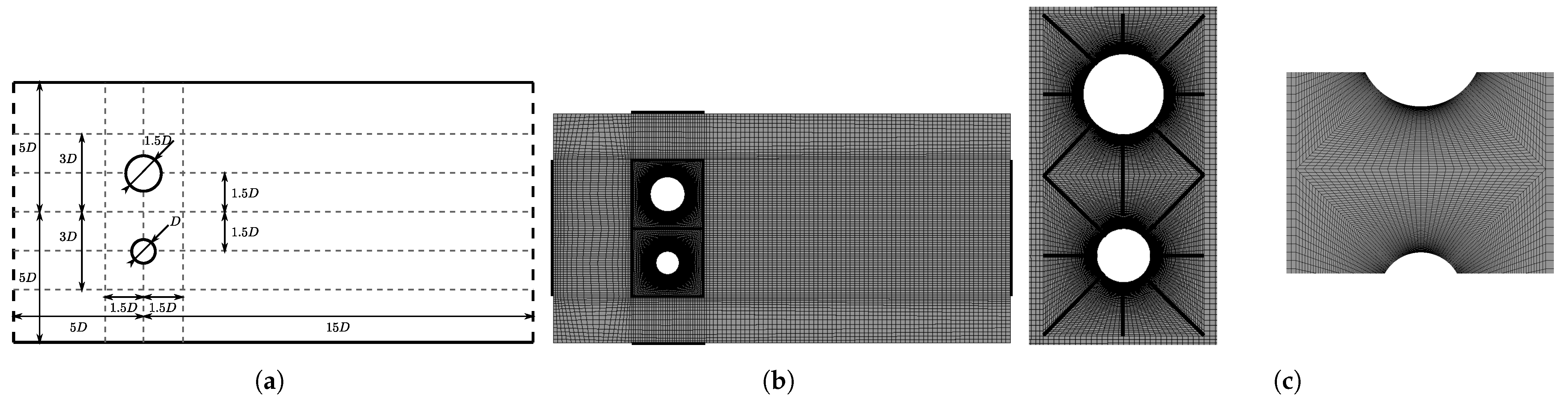
4.1. Geometry, Boundary Conditions, and Mesh

The boundary conditions are the same used for the case of one-cylinder and the geometry is represented in Figure 6a. We now have two cylinders: one with radius D (bottom) and the other with radius $1.5D$ (top). The mesh convergence study was similar to the one presented for the flow around a cylinder, being the estimated relative error of the same order. The chosen mesh now has $\mathrm{23,944}$ elements.

Figure 6b presents a global view of the chosen mesh and Figure 6c shows a zoomed view of the mesh around the two cylinders. The cell size was set to $0.0025$ m along the cylinders’ surface region, $0.01$ m along bold lines of Figure 6b and $0.02$ m on the rest of the domain. The cell size growth rate is $1.2$. Along the bold edges (Figure 6c), a bias type procedure was used with a bias factor of 10. We obtained a mesh with $\mathrm{23,944}$ elements.

4.2. Rheological Properties

For the Newtonian fluid, we have $Re=100$ near to the smaller cylinder with diameter $D=0.1$ m and $Re=150$ near the larger cylinder with diameter $1.5D=0.15$ m. This way, we kept the imposed inlet velocity as $U={10}^{-3}\mathrm{m}·{\mathrm{s}}^{-1}$. For the non-Newtonian power-law, the rheological properties are the same presented in Section 3.2.

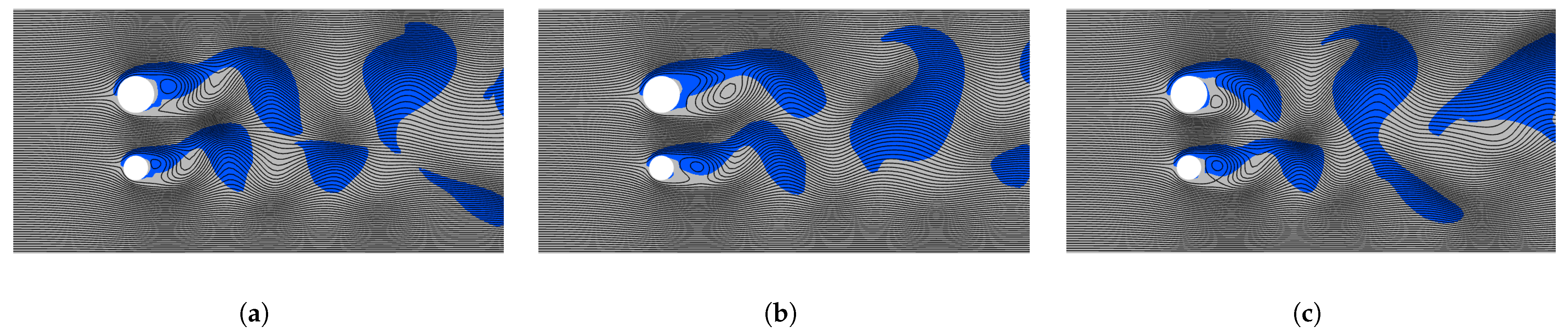
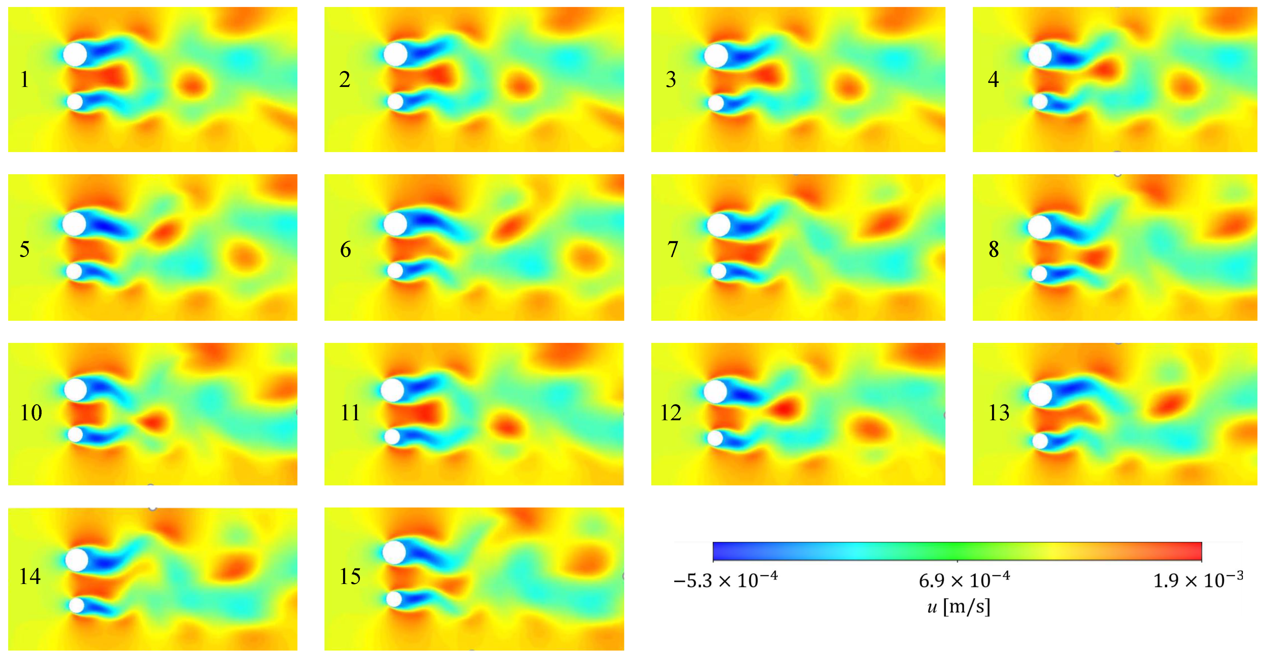
4.3. Results and Discussion

The transient simulation was performed, and the first $10\lambda$ seconds were again neglected to avoid the strong influence of the initial conditions. The subsequent $10\lambda$ seconds of data were then analysed. We considered the same $\delta t_{CFD}$ and $\delta t_{POD}$ of the flow around one cylinder.

Figure 7a–c present the streamlines and the vorticity sign map for the flow around two cylinders, for the Newtonian fluid, and, the power-law fluids with $n=0.7$ and $n=1.3$, respectively. We can see that the oscillatory behaviour downstream the cylinders is perceptible and the vortices detach from each cylinder rear, with different sizes. Later in time, the vortices that arise from both cylinders interact and new structures are formed, where the individual influence of each cylinder is no more clear, when compared to the one-cylinder case. From Equation (8) for $Re=100$ (smaller cylinder), we have $St\approx 0.17$ and consequently the structures behind the cylinder are about six times bigger than the cylinder itself. Near the bigger cylinder, with diameter $1.5D$, a $Re=150$ corresponds to $St\approx 0.18$ and vortices are slightly bigger.

In order to better understand the dynamics of this flow, we provide simulation videos with the flow fields $u,v$ and p (please see the Supplementary Material). Some snapshots/instants of the evolution in time of the velocity component u are shown in Figure 8. The figures are numbered from 1 to 15, with 1 representing $t\approx 0\mathrm{s}$ and 15 representing $t\approx 2.3\mathrm{s}$ of simulation. From instants 1 to 5, the flow in the wake of the cylinders is similar, although the different scales generate different structures that lead to the asynchronous flow verified in instant 6. These asynchronous flow results in the formation of higher velocity structures that detach from the main flow in the wake of the cylinder. This analysis alone is still insufficient to fully understand the influence of the one cylinder over the other. Therefore, we will now present a detailed analysis based on POD, and show that these methods allow one to unveil the origin and evolution of the different structures.

As for the case of one cylinder, we only considered the first 20 eigenvalues and modes. Figure 9a–c show the relative weight of the eigenvalues associated with each mode, for a Newtonian fluid, a power-law fluid with $n=0.7$ and a power-law fluid with $n=1.3$, respectively.

In all figures, we see a fast decrease of the relative weight of the eigenvalues associated with each mode. In Figure 9a, the weight attributed to the first, second and third eigenvalues is $95.7\%$, $1.21\%$ and $0.98\%$, respectively. In Figure 9b, the weights are $97.5\%$, $0.79\%$ and $0.67\%$. In Figure 9c, the weights are $94.5\%$, $1.5\%$ and $1.2\%$.

This leads to the conclusion that with two cylinders, the importance of the first modes is not so clear as in the one-cylinder case. The existence of a second cylinder with different frequencies associated and the interaction of the structures that emerge from the distinct cylinders lead to the use of a higher number of frequencies and modes, to correctly predict/reconstruct the flow.

Table 4. Most important modes (1 to 7) of u, v and p for the flow around two cylinders. For each component u, v and p, we have from left to right: a Newtonian fluid, a power-law fluid with $n=0.7$ and a power-law fluid with $n=1.3$.

	u			v			p
1
2
3
4
5
6
7

shows the most important modes of u, v and p, for the flow around two cylinders (for each component u, v and p, we have from left to right: a Newtonian fluid, a power–law fluid with $n=0.7$ and a power–law fluid with $n=1.3$).

We see that the first mode has the main features of the flow, but without the oscillating components. Mode 1 is in close agreement with the ensemble average (as expected). Notice that the values of u, v and p for mode 1 are symmetrical of what was supposed to happen. This happens because this mode is multiplied by the temporal coefficients that, in this case, are negative. Modes 2 and 3 are related to vortices that detach from the top cylinder, whereas modes 4 and 5 can be associated with the bottom cylinder. In modes 2 and 3, we can see flow structures of the top cylinder in front of the bottom cylinder, and that type of influence is hard to see without a decomposition by modes like we perform in here. Unlike the flow around one cylinder, the modes after mode 5 are not similar by pairs neither easily associated with some meaningful flow structure.

In order to better understand this phenomena,

Table 5. Comparison between the original (first row of images) data versus the partial reconstruction at $t=20\lambda$ (the modes used in the reconstruction are shown in the first column). For each component u, v and p, we have from left to right: a Newtonian fluid, a power-law fluid with $n=0.7$ and a power-law fluid with $n=1.3$.

	u			v			p
2, 3
4, 5
1–3
1–5

shows a comparison between the original data and the partial reconstruction at $t=20\lambda$, for the three fluids (for each component u, v and p, we have from left to right: a Newtonian fluid, a power-law fluid with $n=0.7$ and a power-law fluid with $n=1.3$). From these results, we conclude that the partial reconstruction with just modes 2 and 3 recovers the bigger vortices traveling along the domain associated with the top cylinder. When modes 4 and 5 are considered, we capture the smaller vortices downstream the bottom cylinder (in a short distance from the cylinder). In the reconstruction with the first five modes almost all the structures are perceptible, although slight corrections are missing.

Due to the different vortices that are formed along time and space, the task of finding a direct relationship between the modes and the exact structures is really hard to perform. Although we have plotted the velocity fields obtained for the Newtonian fluid at $t=10\lambda$, $t=15\lambda$ and $t=20\lambda$ seconds (together with the velocity fields obtained for the modes 2 and 3, and, modes 4 and 5). These results are shown in Figure 10.

From Figure 10, it is clear that the relationship between modes 2, 3 and modes 4, 5 and the top and bottom cylinders prevails along time. In addition, we may conclude that the both reconstructions still have information on both cylinders. The isolated vortices are not completely retrieved, but the association is clear. It is also noticeable that, if the spatial characteristics are preserved, the temporal ones are merged. The intensity of each vortex pattern (represented by the vector lengths) is proportional to the vortices at this position in the decomposed dataset. When the velocity components are decomposed, the intensity of the vectors (vector length) coincides with the local averaged kinetic energy.

Notice that the original data for variables u, v and p, with $\mathrm{23,944}$ elements along 400 time steps are saved into a matrix with $\left(3\times \mathrm{23,944}\times 400\right)$ about $28.7$ million values that needs to be stored. Due to computational limitations of the MATLAB software in the calculations of the elements applying the POD method (the same happened for the flow around one cylinder), we only considered one fifth of the elements. The data were saved into a matrix of $\left(3\times 4789\times 400\right)$ about $5.7$ million entries. The reconstruction made with just five modes only needs $\left(3\times 4789\times 5\right)$ storage that is $\mathrm{71,835}$ values. This is a reduction of $98.75\%$ with no significant loss of information, resulting in significant savings.

In Figure 11, an analysis of the frequencies of the modes time coefficients is performed. The Strouhal numbers presented in the figure are calculated considering the frequency with higher energy, the diameter of the bottom cylinder, D, and the mean velocity U.

By Equation (8), the Strouhal number for $Re=100$ is about $0.17$ and for $Re=150$ the Strouhal number is $0.18$. We can relate these predicted Strouhal numbers to the ones presented in Figure 11 for the Newtonian fluid. Therefore, analysing the frequencies of modes 2 and 3, we see that $St=0.155$ and the difference to the predicted Strouhal for the top cylinder (considering the the diameter $1.5D$) is about $30\%$. For modes 4 and 5, we have $St=0.22$ that, when compared with the value predicted by Equation (8) for the bottom cylinder, shows a deviation of about $30\%$.

As in the flow around one cylinder, Figure 11 shows that modes greater than one seam to be organized in pairs, revealing the need for the combination of two structures to correctly model the evolution of the flow structures along the domain.

In Figure 11 we also see that for the three fluids the Strouhal numbers are very similar, meaning that the flow characteristics induced by the two cylinders are more important than the rheology of the fluids.

In Table 4 and Table 5 we saw that modes 2 and 3 were associated with the top cylinder. Thus, taking that into account, we can derive some conclusions related to the Strouhal numbers and how do they relate with the other modes represented in Figure 11. Therefore, we see that modes 6 and 7 have a Strouhal number approximately half the Strouhal number of modes 2 and 3, whereas the Strouhal number of modes 10 and 11 is twice the value obtained for modes 2 and 3. Thus, we conclude that modes 6 and 7 and modes 10 and 11 are related to the same flow structures of modes 2 and 3.

In Figure 11, for the case of a Newtonian fluid, we also notice that the Strouhal number calculated for the second most important frequency of modes 2 and 3 is the Strouhal number associated with modes 4 and 5, and vice versa. This means that the flow structure associated with modes 4 and 5 interferes with the flow structures associated with modes 2 and 3, and vice versa. The same happens to modes 6 and 7 and modes 8 and 9. This means that the flow structures associated with modes 8 and 9 interfere with the flow structure associated with modes 6 and 7, and vice versa.

In Figure 11, for the case of a power-law fluid with $n=0.7$, we also notice that the Strouhal number calculated for the second most important frequency of modes 2 and 3 is the Strouhal number associated with modes 4 and 5 (the flow structure associated with modes 4 and 5 interferes with the flow structure associated with modes 2 and 3, and vice versa), but this relationship is not observed for the other modes. This is due to the use of a different constitutive model for the viscosity.

Finally, in Figure 11, for the power-law fluid with $n=1.3$, we see that the Strouhal number calculated for the second most important frequency of modes 2 and 3 is the Strouhal number associated with modes 4 and 5, but not the other way around. However, for modes 6 and 7, the Strouhal number calculated for the second most important frequency is associated with modes 8 and 9, and vice versa. This means that the flow structure associated with modes 8 and 9 interferes with the flow structures associated with modes 6 and 7, and vice versa. This is again due to the use of a different constitutive model for the viscosity.

In this case we cannot establish a relationship between the Strouhal numbers in the same way as in the flow around one cylinder. Although, visually we know that the different modes are related to the upper or lower cylinder, thus allowing us to use POD to detect and predict flow feature with much less information.

Figure 12a–c show the pairs of time coefficients of consecutive modes, according to frequencies represented in Figure 11 for the Newtonian fluid, the power-law fluid with $n=0.7$ and the power-law fluid with $n=1.3$, respectively.

The oscillatory and alternating behaviour is observed for modes 2 and 3, modes 4 and 5, and modes 6 and 7.

To compare the weights of the modes taking into account the oscillating behaviour, we considered the reference value (19):

$$\overline{\sqrt{{a_1}^2}}+\overline{\sqrt{{a_2}^2+{a_3}^2}}+\overline{\sqrt{{a_4}^2+{a_5}^2}}+\overline{\sqrt{{a_6}^2+{a_7}^2}}.$$

(19)

The modes higher than 7 were not considered due to their small contributions.

For the Newtonian fluid, we see that mode 1, without the oscillatory information, has about $75\%$ of the information in (19), whereas modes 2 and 3 have approximately $11.2\%$ of the information in (19) (referring to $\overline{\sqrt{{a_2}^2+{a_3}^2}}$), modes 4 and 5 have approximately $8\%$ of the information in (19) (referring to $\overline{\sqrt{{a_4}^2+{a_5}^2}}$) and modes 6 and 7 have approximately $6\%$ of the information in (19) (referring to $\overline{\sqrt{{a_6}^2+{a_7}^2}}$).

For the non-Newtonian power-law fluid where $n=0.7$, mode 1, without the oscillatory information, has about $79.5\%$ of the information in (19), whereas modes 2 and 3 have approximately $9.7\%$ of the information in (19) (referring to $\overline{\sqrt{{a_2}^2+{a_3}^2}}$), modes 4 and 5 have approximately $6.5\%$ of the information in (19) (referring to $\overline{\sqrt{{a_4}^2+{a_5}^2}}$) and modes 6 and 7 have approximately $4.3\%$ of the information in (19) (referring to $\overline{\sqrt{{a_6}^2+{a_7}^2}}$). When comparing with the Newtonian fluid, we see that the time weights show a smaller decrease, for pairs of modes after mode 1, but an increase for mode 1. Finally, the non-Newtonian power-law fluid where $n=1.3$, mode 1, without the oscillatory information, has about $72.7\%$ of the information in (19), whereas modes 2 and 3 have approximately $12.1\%$ of the information in (19) (referring to $\overline{\sqrt{{a_2}^2+{a_3}^2}}$), modes 4 and 5 have approximately $8.8\%$ of the information in (19) (referring to $\overline{\sqrt{{a_4}^2+{a_5}^2}}$) and modes 6 and 7 have approximately $6.3\%$ of the information in (19) (referring to $\overline{\sqrt{{a_6}^2+{a_7}^2}}$). When comparing with the Newtonian fluid and with the non-Newtonian power-law where $n=0.7$, we see that the time weights show a smaller decrease on mode 1, but an increase on the pairs of modes after mode 1.

Looking at the results obtained for the Newtonian fluid, the non-Newtonian power-law fluid where $n=0.7$, and with the non-Newtonian power-law fluid where $n=1.3$, we conclude that the first modes are the ones that carry most of the information and with only a few modes we also can reconstruct the simulation.

By using two cylinders with different radii, we get different hidden structures in the flow, and using the modes and the frequencies of the modes time coefficients, some structures can be related to the influence of one cylinder over the other. This gives us a better understanding of the flow.

For ease of understanding of the results presented above, the interested reader can find Supplementary Material, including the videos obtained for the flow around two cylinders (for both the velocity and pressure variables).

5. Conclusions

We performed a detailed study on the flow around a single and two distinct cylinders, by decomposing the von Kármán vortex street data into a generator base that was analysed through the Proper Orthogonal Decomposition. We considered a Newtonian fluid, and two power-law fluids with $n=0.7$ and $n=1.3$. The behaviour obtained for the Newtonian fluid and the power-law fluid with $n=1.3$ (case of one cylinder) is similar, for the range shear rates considered. The power-law fluid with $n=0.7$ shows a more erratic behaviour that could still be captured by the POD method.

We showed that the original POD method can be used to detect and predict flow feature with much less information. A visualization of the influence of each mode on the fluid flow allowed us to infer on the possible reconstruction of the flow features. We also showed the possibility of using the analysis of the frequencies of the temporal coefficients to group modes automatically, or by grouping using visual analysis. By adding an extra cylinder (with a different radius), we obtained different hidden structures in the flow and some of these structures were related to the top cylinder or others related to the Bottom cylinder. A detailed analysis of the flow dynamics revealed the complexity of such flow.

This work aims to inspire other researchers to use the original POD method for decomposing complex flows and better identify meaningful flow structures.

References

1. Lumley, J.L. The Structure of Inhomogenenous Turbulence. Atmos. Turbul. Wave Propag. 1967, 7, 166–178. [Google Scholar]
2. Aubry, N. On the hidden beauty of the proper orthogonal decomposition. Theoret. Comput. Fluid Dyn. 1991, 2, 339–352. [Google Scholar] [CrossRef]
3. Holmes, P.; Lumley, J.L.; Berkooz, G.; Rowley, C.W. Turbulence, Coherent Structures, Dynamical Systems and Symmetry; Cambridge University Press: Cambridge, UK, 2012. [Google Scholar]
4. Berkooz, G.; Holmes, P.; Lumley, J.L. The Proper-Orthogonal Decomposition in the Analysis of Turbulent Flows. Annu. Rev. Fluid Mech. 1993, 25, 539–575. [Google Scholar] [CrossRef]
5. Balajewics, M. A New Approach to Model Order Reduction of the Navier–Stokes Equations. Ph.D. Thesis, Duke University, Durham, NC, USA, 2012. [Google Scholar]
6. Aradag, S.; Siegel, S.; Seidel, J.; Cohen, K.; McLaughlin, T. Filtered POD-based low-dimensional modeling of the 3D turbulent flow behind a circular cylinder. Int. J. Numer. Methods Fluids 2011, 66, 1–16. [Google Scholar] [CrossRef]
7. Ma, X.; Karniadakis, G. A low-dimensional model for simulating three-dimensional cylinder flow. J. Fluid Mech. 2002, 458, 181–190. [Google Scholar] [CrossRef] [Green Version]
8. Towne, A.; Schmidt, O.; Colonius, T. Spectral proper orthogonal decomposition and its relationship to dynamic mode decomposition and resolvent analysis. J. Fluid Mech. 2018, 847, 821–867. [Google Scholar] [CrossRef] [Green Version]
9. Kotu, V.; Deshpande, B. Predictive Analytics and Data Mining: Concepts and Practice with RapidMiner; Elsevier: Waltham, MA, USA, 2015. [Google Scholar]
10. Arntzen, S. Prediction of Flow-Fields by Combining High-Fidelity CFD Data and Machine Learning Algorithms. Master’s Thesis, Delft University of Technology, Delft, The Netherlands, 2019. [Google Scholar]
11. Schäfer, M.; Turek, S.; Durst, F.; Krause, E.; Rannacher, R. Benchmark computations of laminar flow around a cylinder. In Flow Simulation with High-Performance Computers II; Vieweg: Wiesbaden, Germany, 1996; pp. 547–566. [Google Scholar]
12. Bergmann, M.; Cordier, L.; Brancher, J.P. Optimal rotary control of the cylinder wake using proper orthogonal decomposition reduced-order model. Phys. Fluids 2005, 17, 097101. [Google Scholar] [CrossRef]
13. Ping, H.; Zhu, H.; Zhang, K.; Wang, R.; Zhou, D.; Bao, Y.; Han, Z. Wake dynamics behind a rotary oscillating cylinder analyzed with proper orthogonal decomposition. Ocean. Eng. 2020, 218, 108185. [Google Scholar] [CrossRef]
14. Riches, G.; Martinuzzi, R.; Morton, C. Proper orthogonal decomposition analysis of a circular cylinder undergoing vortex-induced vibrations. Phys. Fluids 2018, 30, 105103. [Google Scholar] [CrossRef]
15. Sakai, M.; Sunada, Y.; Imamura, T.; Rinoie, K. Experimental and Numerical Flow Analysis around Circular Cylinders Using POD and DMD. In Proceedings of the 44th AIAA Fluid Dynamics Conference, Atlanta, GA, USA, 16–20 June 2014; Volume 3325. [Google Scholar]
16. Zhang, W.; Chen, C.; Sun, D.J. Numerical simulation of flow around two side-by-side circular cylinders at low Reynolds numbers by a POD-Galerkin spectral method. J. Hydrodyn. Ser. A 2009, 24, 82–88. [Google Scholar]
17. Singha, S.; Nagarajan, K.K.; Sinhamahapatra, K.P. Numerical study of two-dimensional flow around two side-by-side circular cylinders at low Reynolds numbers. Phys. Fluids 2016, 28, 053603. [Google Scholar] [CrossRef]
18. Vitkovicova, R.; Yokoi, Y.; Hyhlik, T. Identification of structures and mechanisms in a flow field by POD analysis for input data obtained from visualization and PIV. Exp. Fluids 2020, 61, 171. [Google Scholar] [CrossRef]
19. Delplace, F.; Leuliet, J.C. Generalized Reynolds number for the flow of power law fluids in cylindrical ducts of arbitrary cross-section. Chem. Eng. J. Biochem. Eng. J. 1995, 56, 33–37. [Google Scholar] [CrossRef]
20. Dhinakaran, S.; Oliveira, M.S.N.; Pinho, F.T.; Alves, M.A. Steady flow of power-law fluids in a 1:3 planar sudden expansion. J. Non-Newton. Fluid Mech. 2013, 198, 48–58. [Google Scholar] [CrossRef] [Green Version]
21. Roshko, A. On the Development of Turbulent Wakes from Vortex Streets. NACA Report 1191; National Advisory Committee for Aeronautics: Washington, DC, USA, 1953. [Google Scholar]
22. Liné, A. Eigenvalue spectrum versus energy density spectrum in a mixing tank. Chem. Eng. Res. Des. 2016, 108, 13–22. [Google Scholar] [CrossRef]
23. Liné, A.; Gabelle, J.C.; Morchain, J.; Anne-Archard, D.; Augier, F. On POD analysis of PIV measurements applied to mixing in a stirred vessel with a shear thinning fluid. Chem. Eng. Res. Des. 2013, 91, 2073–2083. [Google Scholar] [CrossRef] [Green Version]
24. Torres, P.; Gonçalves, N.D.; Fonte, C.P.; Dias, M.M.; Lopes, J.C.; Liné, A.; Santos, R.J. Proper Orthogonal Decomposition and Statistical Analysis of 2D Confined Impinging Jets Chaotic Flow. Chem. Eng. Technol. 2019, 42, 1709–1716. [Google Scholar] [CrossRef]
Figure 1. (a) Geometry of the flow around one cylinder. The left dashed line represents the inlet and the right dashed one the outlet. Mesh of the flow around one cylinder with 23,789 elements: (b) global view with black lines with 10 mm elements; (c) close view around the cylinder.
Fluids 06 00384 g001
Figure 2. Flow around a single cylinder. Streamlines and vorticity sign (blue represents positive values and grey negative values) at t = 20 λ seconds for: (a) Newtonian fluid; (b) non-Newtonian power-law fluid with n = 0.7 ; (c) non-Newtonian power-law fluid with n = 1.3 .
Fluids 06 00384 g002
Figure 3. Flow around a single cylinder. Relative weight of the eigenvalues associated with each mode: (a) Newtonian fluid; (b) power-law fluid with n = 0.7 ; (c) power-law fluid with n = 1.3 .
Fluids 06 00384 g003
Figure 4. Analysis of frequencies of the modes time coefficients for a Newtonian fluid (top), a non-Newtonian power-law fluid where n = 0.7 (middle) and a non-Newtonian power-law fluid where n = 1.3 (bottom).
Fluids 06 00384 g004
Figure 5. Flow around a single cylinder. Pairs of time coefficients of consecutive modes: (a) Newtonian fluid; (b) power-law fluid with n = 0.7 ; (c) power-law fluid with n = 1.3 .
Fluids 06 00384 g005
Figure 6. (a) Geometry of the flow around two cylinders. The left dashed line represents the inlet and the right dashed one the outlet. Mesh of the flow around two cylinders with 23 , 944 elements; (b) global view with black lines with 10 mm elements; (c) close view around and between the cylinders.
Fluids 06 00384 g006
Figure 7. Streamlines and vorticity sign (blue represents positive values and grey negative values) at t = 20 λ for: (a) Newtonian fluid; (b) power-law fluid with n = 0.7 ; (c) power-law fluid with n = 1.3 .
Fluids 06 00384 g007
Figure 8. Evolution, in time, of the first component, u, of the velocity profile. The numbers 1 to 15 establish the order of occurrence, with 1 representing t 0 s and 15 representing t 2.33 s . These instants were extracted from the Supplementary Material provided together with this work.
Fluids 06 00384 g008
Figure 9. Relative weight of the eigenvalues associated with each mode, for: (a) Newtonian fluid; (b) power-law fluid with n = 0.7 ; (c) power-law fluid with n = 1.3 .
Fluids 06 00384 g009
Figure 10. Velocity fields obtained for the Newtonian fluid at t = 10 λ , t = 15 λ and t = 20 λ seconds (together with the velocity fields obtained for the modes 2 and 3, and, modes 4 and 5).
Fluids 06 00384 g010
Figure 11. Analysis of frequencies of the modes time coefficients for a Newtonian fluid (top), a non-Newtonian power-law fluid where n = 0.7 (middle) and a non-Newtonian power-law fluid where n = 1.3 (bottom).
Fluids 06 00384 g011
Figure 12. Pairs of time coefficients of consecutive modes: (a) Newtonian fluid; (b) power-law fluid with n = 0.7 ; (c) power-law fluid with n = 1.3 .
Fluids 06 00384 g012