Modeling Acoustic Cavitation Using a Pressure-Based Algorithm for Polytropic Fluids

Abstract
:1. Introduction
2. Governing Equations
3. Polytropic Closure
4. Numerical Framework
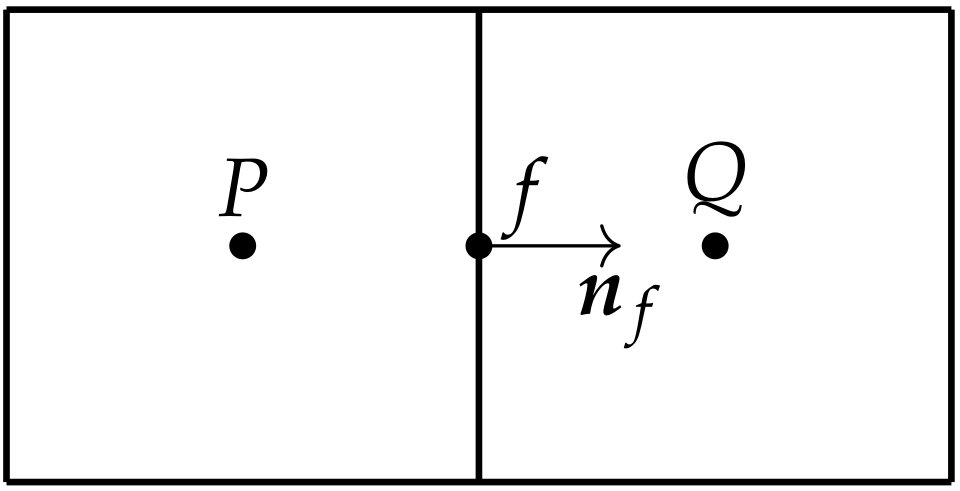
4.1. Finite-Volume Discretization
4.2. Advecting Velocity
4.3. Discretized Governing Equations
4.4. Solution Procedure
5. Interface Treatment
5.1. Interface Advection
5.2. Fluid Properties
6. Results
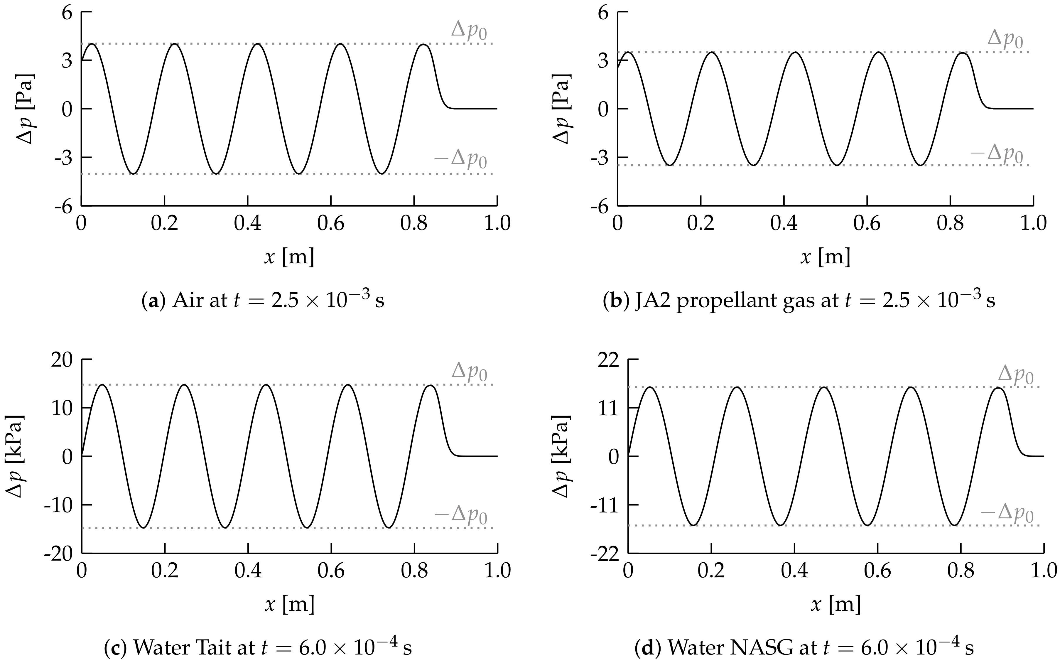
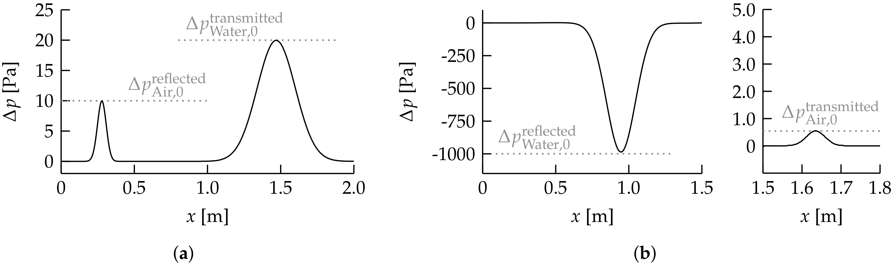
6.1. Acoustic Waves
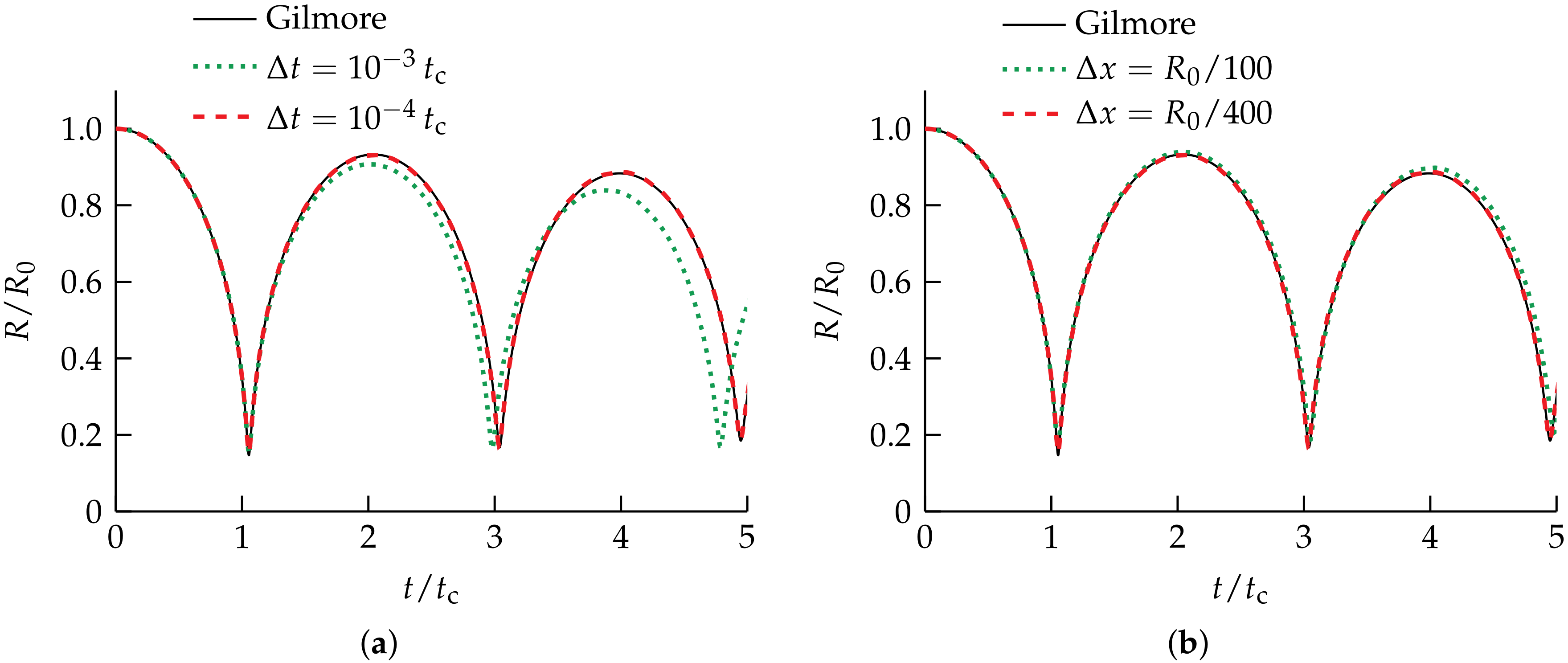
6.2. Rayleigh Collapse
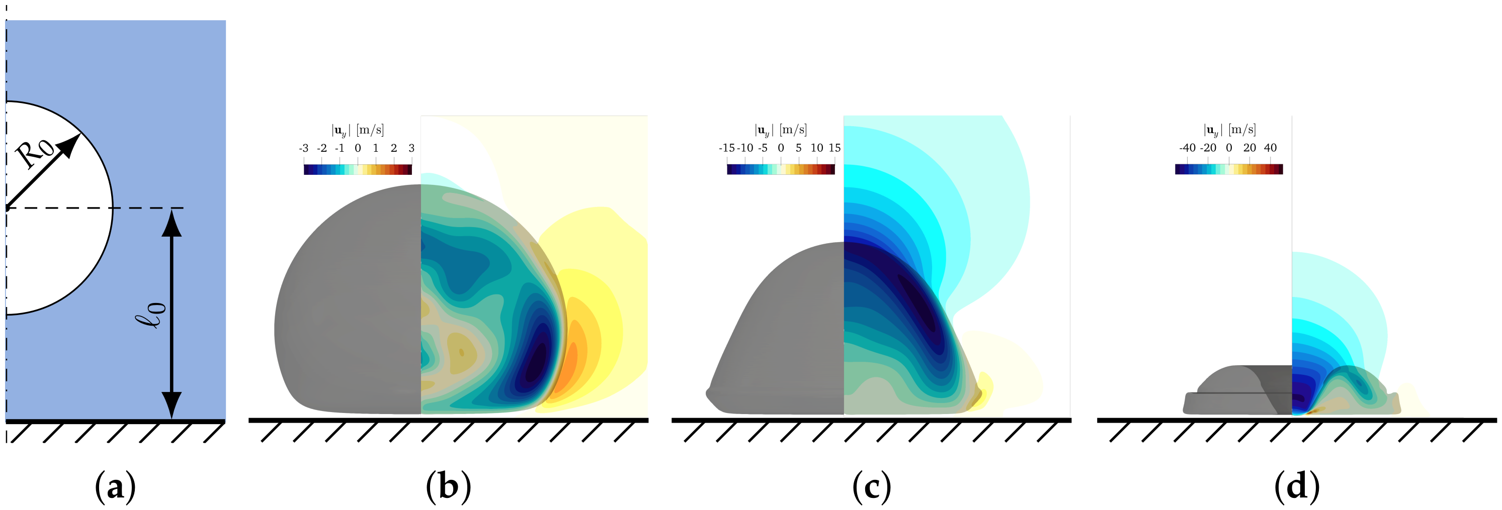
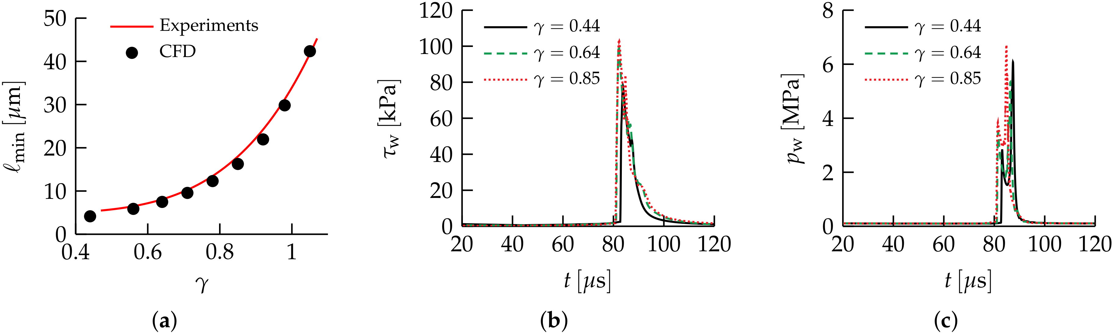
6.3. Wall-Bounded Cavitation
7. Conclusions
Author Contributions
Funding
Acknowledgments
Conflicts of Interest
References
- Leighton, T.G. The Acoustic Bubble; Academy Press: London, UK, 1994. [Google Scholar]
- Reuter, F.; Mettin, R. Mechanisms of Single Bubble Cleaning. Ultrason. Sonochem. 2016, 29, 550–562. [Google Scholar] [CrossRef] [PubMed]
- Cavitation in Biomedicine; Wan, M.; Feng, Y.; ter Haar, G. (Eds.) Springer: Dordrecht, The Netherlands, 2015. [Google Scholar] [CrossRef]
- Tovar, A.R.; Patel, M.V.; Lee, A.P. Lateral Air Cavities for Microfluidic Pumping with the Use of Acoustic Energy. Microfluid. Nanofluidics 2011, 10, 1269–1278. [Google Scholar] [CrossRef] [Green Version]
- Rabaud, D.; Thibault, P.; Mathieu, M.; Marmottant, P. Acoustically Bound Microfluidic Bubble Crystals. Phys. Rev. Lett. 2011, 106. [Google Scholar] [CrossRef] [PubMed]
- Rayleigh, L. On the Pressure Developed in a Liquid during the Collapse of a Spherical Cavity. Philos. Mag. 1917, 34, 94–98. [Google Scholar] [CrossRef]
- Lauterborn, W.; Kurz, T. Physics of Bubble Oscillations. Rep. Prog. Phys. 2010, 73, 106501. [Google Scholar] [CrossRef]
- Plesset, M.S. The Dynamics of Cavitation Bubbles. J. Appl. Mech. 1949, 16, 277–282. [Google Scholar] [CrossRef]
- Gilmore, F.R. The Growth or Collapse of a Spherical Bubble in a Viscous Compressible Liquid; Technical Report No. 26-4; California Institute of Technology: Pasadena, CA, USA, 1952. [Google Scholar]
- Keller, J.B.; Miksis, M. Bubble Oscillations of Large Amplitude. J. Acoust. Soc. Am. 1980, 68, 628–633. [Google Scholar] [CrossRef] [Green Version]
- Lechner, C.; Koch, M.; Lauterborn, W.; Mettin, R. Pressure and Tension Waves from Bubble Collapse near a Solid Boundary: A Numerical Approach. J. Acoust. Soc. Am. 2017, 142, 3649–3659. [Google Scholar] [CrossRef]
- Zeng, Q.; Gonzalez-Avila, S.R.; Dijkink, R.; Koukouvinis, P.; Gavaises, M.; Ohl, C.D. Wall Shear Stress from Jetting Cavitation Bubbles. J. Fluid Mech. 2018, 846, 341–355. [Google Scholar] [CrossRef] [Green Version]
- Pan, S.; Adami, S.; Hu, X.; Adams, N.A. Phenomenology of Bubble-Collapse-Driven Penetration of Biomaterial-Surrogate Liquid-Liquid Interfaces. Phys. Rev. Fluids 2018, 3, 114005. [Google Scholar] [CrossRef] [Green Version]
- Goncalves, E.; Hoarau, Y.; Zeidan, D. Simulation of Shock-Induced Bubble Collapse Using a Four-Equation Model. Shock Waves 2019, 29, 221–234. [Google Scholar] [CrossRef] [Green Version]
- Denner, F.; van Wachem, B. Numerical Modelling of Shock-Bubble Interactions Using a Pressure-Based Algorithm without Riemann Solvers. Exp. Comput. Multiph. Flow 2019, 1, 271–285. [Google Scholar] [CrossRef] [Green Version]
- Wilson, C.T.; Hall, T.L.; Johnsen, E.; Mancia, L.; Rodriguez, M.; Lundt, J.E.; Colonius, T.; Henann, D.L.; Franck, C.; Xu, Z.; et al. Comparative Study of the Dynamics of Laser and Acoustically Generated Bubbles in Viscoelastic Media. Phys. Rev. E 2019, 99, 043103. [Google Scholar] [CrossRef] [PubMed] [Green Version]
- Plesset, M.S.; Prosperetti, A. Bubble Dynamics and Cavitation. Annu. Rev. Fluid Mech. 1977, 9, 145–185. [Google Scholar] [CrossRef]
- Denner, F.; Evrard, F.; van Wachem, B. Conservative Finite-Volume Framework and Pressure-Based Algorithm for Flows of Incompressible, Ideal-Gas and Real-Gas Fluids at All Speeds. J. Comput. Phys. 2020, 409, 109348. [Google Scholar] [CrossRef] [Green Version]
- Chorin, A.J. Numerical Solution of the Navier-Stokes Equations. Math. Comput. 1968, 22, 745. [Google Scholar] [CrossRef]
- Bell, J.B.; Colella, P.; Glaz, H.M. A Second-Order Projection Method for the Incompressible Navier-Stokes Equations. J. Comput. Phys. 1989, 85, 257–283. [Google Scholar] [CrossRef] [Green Version]
- Patankar, S.; Spalding, D. A Calculation Procedure for Heat, Mass and Momentum Transfer in Three-Dimensional Parabolic Flows. Int. J. Heat Mass Transf. 1972, 15, 1787–1806. [Google Scholar] [CrossRef]
- Miller, S.T.; Jasak, H.; Boger, D.A.; Paterson, E.G.; Nedungadi, A. A Pressure-Based, Compressible, Two-Phase Flow Finite Volume Method for Underwater Explosions. Comput. Fluids 2013, 87, 132–143. [Google Scholar] [CrossRef]
- Koch, M.; Lechner, C.; Reuter, F.; Köhler, K.; Mettin, R.; Lauterborn, W. Numerical Modeling of Laser Generated Cavitation Bubbles with the Finite Volume and Volume of Fluid Method, Using OpenFOAM. Comput. Fluids 2016, 126, 71–90. [Google Scholar] [CrossRef]
- Darwish, M.; Sraj, I.; Moukalled, F. A Coupled Finite Volume Solver for the Solution of Incompressible Flows on Unstructured Grids. J. Comput. Phys. 2009, 228, 180–201. [Google Scholar] [CrossRef]
- Chen, Z.; Przekwas, A.J. A Coupled Pressure-Based Computational Method for Incompressible/Compressible Flows. J. Comput. Phys. 2010, 229, 9150–9165. [Google Scholar] [CrossRef]
- Denner, F.; van Wachem, B. Fully-Coupled Balanced-Force VOF Framework for Arbitrary Meshes with Least-Squares Curvature Evaluation from Volume Fractions. Numer. Heat Transf. Part B Fundam. 2014, 65, 218–255. [Google Scholar] [CrossRef] [Green Version]
- Darwish, M.; Moukalled, F. A Fully Coupled Navier-Stokes Solver for Fluid Flow at All Speeds. Numer. Heat Transf. Part B Fundam. 2014, 65, 410–444. [Google Scholar] [CrossRef]
- Xiao, C.N.; Denner, F.; van Wachem, B. Fully-Coupled Pressure-Based Finite-Volume Framework for the Simulation of Fluid Flows at All Speeds in Complex Geometries. J. Comput. Phys. 2017, 346, 91–130. [Google Scholar] [CrossRef]
- Denner, F. Fully-Coupled Pressure-Based Algorithm for Compressible Flows: Linearisation and Iterative Solution Strategies. Comput. Fluids 2018, 175, 53–65. [Google Scholar] [CrossRef] [Green Version]
- Denner, F.; Xiao, C.N.; van Wachem, B. Pressure-Based Algorithm for Compressible Interfacial Flows with Acoustically-Conservative Interface Discretisation. J. Comput. Phys. 2018, 367, 192–234. [Google Scholar] [CrossRef]
- Hirt, C.; Nichols, B. Volume of Fluid (VOF) Method for the Dynamics of Free Boundaries. J. Comput. Phys. 1981, 39, 201–225. [Google Scholar] [CrossRef]
- Le Métayer, O.; Saurel, R. The Noble-Abel Stiffened-Gas Equation of State. Phys. Fluids 2016, 28, 046102. [Google Scholar] [CrossRef] [Green Version]
- Toro, E.F. Riemann Solvers and Numerical Fluid Dynamics: A Practical Introduction, 3rd ed.; Springer: Berlin/Heidelberg, Germany, 2009. [Google Scholar]
- Le Métayer, O.; Massoni, J.; Saurel, R. Élaboration des lois d’état d’un liquide et de sa vapeur pour les modèles d’écoulements diphasiques. Int. J. Therm. Sci. 2004, 43, 265–276. [Google Scholar] [CrossRef]
- Bartholomew, P.; Denner, F.; Abdol-Azis, M.; Marquis, A.; van Wachem, B. Unified Formulation of the Momentum-Weighted Interpolation for Collocated Variable Arrangements. J. Comput. Phys. 2018, 375, 177–208. [Google Scholar] [CrossRef]
- Denner, F.; van Wachem, B. TVD Differencing on Three-Dimensional Unstructured Meshes with Monotonicity-Preserving Correction of Mesh Skewness. J. Comput. Phys. 2015, 298, 466–479. [Google Scholar] [CrossRef] [Green Version]
- Rhie, C.M.; Chow, W.L. Numerical Study of the Turbulent Flow Past an Airfoil with Trailing Edge Separation. AIAA J. 1983, 21, 1525–1532. [Google Scholar] [CrossRef]
- Denner, F.; van Wachem, B. Numerical Time-Step Restrictions as a Result of Capillary Waves. J. Comput. Phys. 2015, 285, 24–40. [Google Scholar] [CrossRef] [Green Version]
- Karimian, S.M.H.; Schneider, G.E. Pressure-Based Computational Method for Compressible and Incompressible Flows. J. Thermophys. Heat Transf. 1994, 8, 267–274. [Google Scholar] [CrossRef]
- Kunz, R.; Cope, W.; Venkateswaran, S. Development of an Implicit Method for Multi-Fluid Flow Simulations. J. Comput. Phys. 1999, 152, 78–101. [Google Scholar] [CrossRef] [Green Version]
- Balay, S.; Gropp, W.; McInnes, L.C.; Smith, B.F. Efficient Management of Parallelism in Object Oriented Numerical Software Libraries. In Modern Software Tools in Scientific Computing; Arge, E., Bruasat, A., Langtangen, H., Eds.; Birkhäuser Press: Boston, MA, USA, 1997; pp. 163–202. [Google Scholar]
- Balay, S.; Abhyankar, S.; Adams, M.F.; Brown, J.; Brune, P.; Buschelman, K.; Dalcin, L.; Eijkhout, V.; Gropp, W.D.; Kaushik, D.; et al. PETSc Web Page. 2020. Available online: http://www.mcs.anl.gov/petsc (accessed on 13 April 2020).
- Balay, S.; Abhyankar, S.; Adams, M.F.; Brown, J.; Brune, P.; Buschelman, K.; Dalcin, L.; Eijkhout, V.; Kaushik, D.; Knepley, M.G.; et al. PETSc Users Manual; Technical Report ANL-95/11 - Revision 3.8; Argonne National Laboratory: Lemont, IL, USA, 2017. [Google Scholar]
- Ubbink, O.; Issa, R. A Method for Capturing Sharp Fluid Interfaces on Arbitrary Meshes. J. Comput. Phys. 1999, 153, 26–50. [Google Scholar] [CrossRef] [Green Version]
- Gopala, V.; van Wachem, B. Volume of Fluid Methods for Immiscible-Fluid and Free-Surface Flows. Chem. Eng. J. 2008, 141, 204–221. [Google Scholar] [CrossRef]
- Denner, F. Wall Collision of Deformable Bubbles in the Creeping Flow Regime. Eur. J. Mech. B Fluids 2018, 70, 36–45. [Google Scholar] [CrossRef]
- Anderson, J.D. Modern Compressible Flow: With a Historical Perspective; McGraw-Hill: New York, NY, USA, 2003. [Google Scholar]
- Johnston, I. The Noble-Abel Equation of State: Thermodynamic Derivations for Ballistics Modelling; Technical Report Technical Report DSTO-TN-0670; Defence Science and Technology Organisation: Edinburgh, Australia, 2005. [Google Scholar]
- Lauterborn, W.; Lechner, C.; Koch, M.; Mettin, R. Bubble Models and Real Bubbles: Rayleigh and Energy-Deposit Cases in a Tait-Compressible Liquid. IMA J. Appl. Math. 2018, 83, 556–589. [Google Scholar] [CrossRef]
- Schmidmayer, K.; Bryngelson, S.H.; Colonius, T. An Assessment of Multicomponent Flow Models and Interface Capturing Schemes for Spherical Bubble Dynamics. J. Comput. Phys. 2020, 402, 109080. [Google Scholar] [CrossRef] [Green Version]
- Reuter, F.; Kaiser, S.A. High-Speed Film-Thickness Measurements between a Collapsing Cavitation Bubble and a Solid Surface with Total Internal Reflection Shadowmetry. Phys. Fluids 2019, 31, 097108. [Google Scholar] [CrossRef]
- Ohl, C.; Kurz, T.; Geisler, R.; Lindau, O.; Lauterborn, W. Bubble Dynamics, Shock Waves and Sonoluminescence. Philos. Trans. R. Soc. Lond. Ser. A Math. Phys. Eng. Sci. 1999, 357, 269–294. [Google Scholar] [CrossRef]
- Vogel, A.; Busch, S.; Parlitz, U. Shock Wave Emission and Cavitation Bubble Generation by Picosecond and Nanosecond Optical Breakdown in Water. J. Acoust. Soc. Am. 1996, 100, 148–165. [Google Scholar] [CrossRef]
- Supponen, O.; Obreschkow, D.; Kobel, P.; Tinguely, M.; Dorsaz, N.; Farhat, M. Shock Waves from Nonspherical Cavitation Bubbles. Phys. Rev. Fluids 2017, 2, 093601. [Google Scholar] [CrossRef] [Green Version]


| Fluid | b [m kg] | [Pa] | |
|---|---|---|---|
| Air | 0 | 0 | |
| JA2 propellant gas [48] | 0 | ||
| Water Tait [23] | 0 | ||
| Water NASG [32] |
| Fluid | f [s] | [kg m] | [m s] | [m] | [Pa] | [m] | [Pa] |
|---|---|---|---|---|---|---|---|
| Air | 1750 | ||||||
| JA2 propellant gas [48] | 1750 | ||||||
| Water Tait [23] | 7500 | 1000 | |||||
| Water NASG [32] | 7500 | 1000 |
© 2020 by the authors. Licensee MDPI, Basel, Switzerland. This article is an open access article distributed under the terms and conditions of the Creative Commons Attribution (CC BY) license (http://creativecommons.org/licenses/by/4.0/).
Share and Cite
Denner, F.; Evrard, F.; van Wachem, B. Modeling Acoustic Cavitation Using a Pressure-Based Algorithm for Polytropic Fluids. Fluids 2020, 5, 69. https://doi.org/10.3390/fluids5020069
Denner F, Evrard F, van Wachem B. Modeling Acoustic Cavitation Using a Pressure-Based Algorithm for Polytropic Fluids. Fluids. 2020; 5(2):69. https://doi.org/10.3390/fluids5020069
Chicago/Turabian StyleDenner, Fabian, Fabien Evrard, and Berend van Wachem. 2020. "Modeling Acoustic Cavitation Using a Pressure-Based Algorithm for Polytropic Fluids" Fluids 5, no. 2: 69. https://doi.org/10.3390/fluids5020069