Assessing and Forecasting the Long-Term Impact of the Global Financial Crisis on New Car Sales in South Africa

Abstract

In both developed and developing nations, with South Africa (SA) being one of the latter, the motor vehicle industry is one of the most important sectors. The SA automobile industry was not unaffected by the 2007/2008 global financial crisis (GFC). This study aims to assess the impact of the GFC on new car sales in SA through statistical modeling, an impact that has not previously been investigated or quantified. The data obtained indicate that the optimal model for assessing the aforementioned impact is the SARIMA (0,1,1)(0,0,2)₁₂ model. This model’s suitability was confirmed using Akaike information criterion (AIC) and Bayesian information criterion (BIC), as well as the root mean square error (RMSE) and the mean absolute percentage error (MAPE). An upward trend is projected for new car sales in SA, which has positive implications for SA and its economy. The projections indicate that the new car sales rate has increased and has somewhat recovered, but it has not yet reached the levels expected had the GFC not occurred. This shows that SA’s new car industry has been negatively and severely impacted by the GFC and that the effects of the latter still linger today. The findings of this study will assist new car manufacturing companies in SA to better understand their industry, to prepare for future negative shocks, to formulate potential policies for stocking inventories, and to optimize marketing and production levels. Indeed, the information presented in this study provides talking points that should be considered in future government relief packages.

1. Introduction

The automotive sector is a critical industry in most developed and developing countries [1]. After 1994 and the end of apartheid, South Africa (SA), a developing country, has seen rapid economic growth [2]. The average yearly gross domestic product (GDP) growth rate for SA rose from 3.6% between 2000 and 2003 to 5.1% between 2004 and 2007 [3].

More labor-intensive economic sectors, including manufacturing (particularly automotive), mining, trade, and construction, faced high unemployment rates during the global financial crisis (GFC) of 2007/2008 [4]. Global consumer demand declined, and, to make matters worse, SA began to experience severe energy shortages, which had an adverse effect on the manufacturing sector, particularly the automotive industry. The value added by SA’s manufacturing decreased by 12.2% in 2009 [5]. Consequently, large decreases were experienced in the output of the automobile industry (34%), furniture industry (20%), and textile and apparel sector (14.6%). This had a negative impact on the country’s economy.

The SA automobile sector generated 6.8% of the nation’s GDP in 2018 (4.3% manufacturing and 2.5% retail) and directly employed about 110,000 people [6]. In 2019, the automobile industry contributed 300,000 jobs (100,000 directly in the manufacturing of vehicles and components and 200,000 indirectly). The sector contributed 6.4% to the national GDP and constituted 19% of the total manufacturing output [7].

According to [7], SA is the African continent’s top vehicle manufacturer (54.3%), with 9 major original equipment manufacturers (OEMs) producing 600,000 vehicles per annum as of 2019; these serve both the domestic (40%) and export markets (60%). As one of SA’s fastest-growing sectors, the automotive sector has long played a vital role in the country’s economy. In 2021, it was regarded as the cornerstone of the national industrial foundation and the main manufacturing sector of the nation’s economy. The automobile industry contributed 4.3% to GDP (2.4% manufacturing and 1.9% retail) in 2021 [8].

During the GFC, not only SA but other countries worldwide were affected by decreasing car sales. As per [9], the automotive industry, along with several other sectors, was significantly affected in 2008 and 2009. Tightening global financing conditions resulted in a nearly 25% drop in global vehicle sales from their peak in April 2008 to their trough in January 2009. Bai [10] reported that the financial and economic crisis had a strong negative effect on the automotive industry in Germany, with a 31% decline in passenger car sales and a 59% decrease in commercial vehicle sales by the end of 2009. The Chinese automotive industry experienced a 15% decline in its total automobile sales volume in 2009. In the first half of 2020, new car sales in European Union member states experienced an average decline of 36%, as reported by [11], due to yet another shock, namely, the COVID-19 pandemic.

Reliable automotive projections play a crucial role in strategic planning. SA reported a significant drop in new car sales between 2007 and 2008, reflecting the impact of the GFC on vehicle manufacturers worldwide [12]. The decline in new car sales and other sectors of the economy caused significant job losses, with damaging effects on workers’ living standards. Its state-of-the-art car assemblies make SA the economic powerhouse of southern Africa. Understanding how SA’s automotive industry was affected by the economic shock of the GFC provides valuable insights into similar economic shocks, including those experienced during the COVID-19 pandemic. These insights afford investors, customers, and other stakeholders an opportunity to understand the industry’s vulnerabilities, challenges, and opportunities during similar economic shocks. When South Africa sneezes, the rest of the southern African economic region catches a cold. In other words, the economy of all of southern Africa is affected when SA’s economy suffers.

The accurate forecasting of automotive sales helps dealers to dynamically change their marketing tactics and, in the case of a financial crisis, to make wise decisions for both the wider economy and the transportation sector. According to [13], accurate sales predictions strengthen the competitive edge of vehicle manufacturers in their efforts to optimize their production planning processes. Sales forecasting is crucial for the implementation of sustainable business strategies in the automotive sector. Any financial crisis or economic instability in a country influences purchase decisions related to cars and car products [14].

The aim of this study is to assess the effect of the GFC on new car sales in SA through the use of statistical modeling. The study hypothesizes that the GFC had negative long-term effects on new car sales in SA. Therefore, the researchers consider new car sale trends in SA before, during, and after the GFC. Scholarship regarding the effect of the GFC on new car sales on the African continent, and in SA in particular, is negligible. Understanding how much the SA automotive industry was impacted by the GFC, and how long the industry took (or will take) to recover from the repercussions, is crucial in preparing for future shocks.

The originality of this research should be viewed in the context of applying an already established statistical methodology to provide new insights into the complex relationship between global financial events and local market conditions, and by demonstrating the impact of a shock on new car sales in SA. The approach is used as a tool for understanding and predicting economic trends in Southern Africa based on the existing data. This study aims to fill an important gap in the existing scholarship, namely investigating the effect of an external shock, the GFC, on new car sales in SA. The study also serves as a frame of reference for similar research on the impact of the financial crisis either on other industries in SA, or in other neighboring countries.

Makatjane and Moroke [15] projected car sales in SA using both the seasonal autoregressive integrated moving average (SARIMA) and Holt–Winters models but did not specifically consider the effect of the GFC shock. Statistical models are capable of generating accurate short- and long-term motor vehicle sales forecasts. This allows firms to identify market demand patterns and improve market performance, minimize losses, determine product development strategies, and plan manufacturing and marketing policies more efficiently in anticipation of similar shocks in future.

Using ARIMA models for predicting car sales has been effective, even in the presence of anomalies, as demonstrated by several studies ([15,16,17,18,19]). However, [20] found that SARIMA models are superior in cases where seasonal unevenness is evident in the data; SARIMA models can also extract linear relationships within time series data, making it a suitable choice for this study. Studies by [21,22,23] further reinforced the usefulness of SARIMA models for prediction purposes. Machine learning algorithms have gained popularity [24], highlighting the need for a multi-phase, complex process to address data leakage problems. The SARIMA model is the preferred choice for this study since it is said to be more effective than most models, with the latter including exponential smoothing techniques [25].

2. Literature Review

Several authors have used the Box–Jenkins approach to forecast automotive sales ([17,26,27]). Common methods used for new car sales forecasting include time series, linear regression, machine learning, and grey forecasting methods. Autoregressive moving average (ARMA) and grey prediction are often the forecasting methods of choice [14]. In SA [15], monthly car sales are mostly forecast by using both the SARIMA and Holt–Winters models. In terms of short-term seasonal auto sales forecasting accuracy, the Holt–Winters model performed better than the SARIMA model.

In Indonesia [26], the ARIMA (2,1,2) and ARIMA (1,1,0) models were used to forecast new car and motorcycle sales, respectively. The results were important in assessing the effect of cars and motorcycles on traffic jams and accidents, as well as air pollution, in order to draft better policies.

The naïve method (NM), simple moving average (SMA), weighted moving average (WMA), simple linear regression (SLR), exponential smoothing (ES), Holt–Winter linear trend, autoregression (AR), ARMA, and ARIMA models were used in India [1] to compare the forecasted demand for vehicles. The Holt–Winter linear trend model was considered the most suitable. However, the modeling was conducted without considering shocks such as a GFC; therefore, the latter is considered in the current study. Shakti et al. [17] used an SARIMA(0,1,1)(0,1,1)₁₂ model to predict 5-year tractor sales for the Mahindra Tractors Company in India. The forecasted average increase in future sales meant an improvement in the country’s GDP, and thus the economy. Such forecasts are at best true/correct if no shocks, such as the GFC experienced during 2007/2008, occur.

Pherwani and Kamath [18] concluded that sales forecasting is a crucial element in successful business management. The authors forecasted the total car sales in India using an ARIMA (1,1,0) model and concluded that their findings could guide motor vehicle companies to cover expenses and decide both employee wages and stocking inventory. The same Box–Jenkins methodology was used by [28] in India to model and predict automobile sales because of their significant impact on the economy through trade flows. However, the authors did not consider the impact of the GFC on car sales in their study. The current research aims to fill an important gap by investigating the effect of this external shock (the GFC) on new car sales, forecasting and providing information/data-based recommendations for inventory management, and other business operations in the automotive industry.

Chen [27] predicted Chinese automotive demand with the Box–Jenkins approach (an ARIMA model) using monthly data. The conclusion was that the ARIMA model generates better forecasts that could aid government in drafting automobile industry policies, as well as automobile enterprises in planning their output. Qu et al. [14] adopted the support vector regression (SVR) model to predict the monthly sales of automobiles in the Chinese car segment. The proposed grey wolf optimizer–support vector regression (GWO-SVR) model fitted the data well. Unlike the Box–Jenkins approach, the GWO-SVR approach is computationally expensive; it requires a significant number of computational resources and time to train and tune the model, especially when dealing with large amounts of data [29], such as with new car sales. The GWO-SVR also lacks interpretability as it uses machine learning techniques that do not provide clear insights into the underlying relationships between variables. Conversely, the ARIMA is a well-established time series model that provides interpretable coefficients that can help explain the relationship between variables.

Kaya and Yildirim [30] used an eight-layer deep neural network (DNN) model to forecast automobile sales. Several variables, such as the consumer confidence index (CCI), the exchange rate, the GDP, and the consumer price index (CPI), were considered. The authors recommend the use of their approach on various sales prediction problems. However, DNN models can be more challenging to use due to their high cost and the need for optimal architecture and hyper-parameter tuning, as noted by [31,32]. Furthermore, DNN models are more suitable to use with a large, homogeneous dataset with multiple observations, according to [33]. For a single variable such as new car sales, SARIMA models can lead to a higher forecasting accuracy and are therefore the preferred choice in this study.

Fantazzini and Toktamysova [34] used multivariate models, drawing on economic variables, and Google online search data to forecast Germany’s monthly car sales. The conclusion was that the models, which included Google search data, outperform other competing car models. Such models can, however, be very complicated and subjective. In multivariate models, variable selection is difficult and subjective, which may lead to overfitting and poor forecasting performance. Thus, the use of ARIMA models that do not require the selection of relevant predictors becomes important.

Kim et al. [25] forecasted offline retail sales during the COVID-19 pandemic period in South Korea by comparing ARIMA to several ETS methods. The conclusion was that the SARIMA (2,0,2)(1,0,0)₁₂, ARIMA (1,0,1)(0,0,0)₁₂, and ARIMA (2,0,3)(0,0,1)₁₂ models were the best fit for retail sales in fashion, cosmetics, and sports categories, respectively, when compared to the naïve seasonal and Holt–Winter additive models. The forecasts showed that sales in the fashion retail category were increasing gradually, with sales in the cosmetics and sports retail categories increasing at a faster rate. The S/ARIMA models were better forecasting models than the ETS models, hence their adoption in the current study.

The simple and flexible Box–Jenkins approach is used in this paper to forecast new car sales in SA. Its suitability relies on its accuracy in forecasting, as well as its flexibility and adaptability to a wide range of time series data, such as new car sales. Brito et al. [35] concluded that the SARIMA models are more flexible in their application and more accurate in generating quality results.

3. Methodology

In this section, the forecasting methods used in the study are explained. The Box–Jenkins [36] methodology is employed in modeling and forecasting new car sales in SA. The ARIMA and SARIMA models are part of the Box–Jenkins approach.

3.1. ARIMA/SARIMA Models

The Box–Jenkins approach involves, firstly, the model identification stage, where the appropriate order of the model is identified through the use of both the autocorrelation function (ACF) and the partial autocorrelation function (PACF). An ARIMA model can be presented as an ARIMA (p,d,q) model, where p is the AR order, which allows the method to incorporate past values in forecasting future values, d is the number of nonseasonal differences needed to achieve stationarity, and q is the MA order which relies on the number of lagged forecast errors in obtaining the forecast values. When the data are not seasonal, the ARIMA (p,d,q) model is appropriate and is represented as:

$$\varphi \left(B\right){(1-B)}^d{Y}_t=c+\theta \left(B\right){\epsilon }_t,$$

(1)

where $B$ is the backward shift operator (${B^{d}Y}_t=Y_{t-d}$), $c$ is a constant term, ${\epsilon }_t~iid N(0,{\sigma }_t^2)$, and ${\sigma }_t^2$ is the error variance term. $Y_t$ is new car sales and $\varphi \left(B\right)$ and $\theta \left(B\right)$ are polynomials of order p and q, respectively.

When the data exhibit seasonality, an SARIMA (p,d,q)(P,D,Q)_s model is possible, and the extra terms are denoted as follows: P is the seasonal AR order, D is the seasonal differencing order, Q is the seasonal MA order, and s denotes the seasonality (s = 12 for monthly data). The following is a representation of an SARIMA (p,d,q) (P,D,Q)_s model:

$$\mathsf{\Phi }\left(B^s\right)\varphi \left(B\right){(1-B^s)}^D{(1-B)}^d{Y}_t=a+\mathsf{\Theta }\left(B^s\right)\theta \left(B\right){\epsilon }_t,$$

(2)

where $\mathsf{\Phi }\left(B^s\right)$ and $\mathsf{\Theta }\left(B^s\right)$ are polynomials of orders P and Q, respectively. The maximum likelihood estimator (MLE) method is used to generate optimal model parameters. When choosing the best model, the Akaike information criterion (AIC) and Bayesian information criterion (BIC) are used. The AIC can be written as:

$$\mathrm{AIC}=-2\log \left(L\right)+2m,$$

(3)

where L is the likelihood function and m is the number of model parameters, as indicated by [37]. The BIC is given as:

$$\mathrm{BIC}=-2\log \left(L\right)+2m\log \left(n\right),$$

(4)

where L is the likelihood function and m and n are the number of model parameters and observations, respectively.

3.2. Time Series Decomposition and Stationarity

Data decomposition is conducted to elucidate some of the time series’ characteristics. To model new car sales using the Box–Jenkins approach, the sales are transformed to make them stationary. A stationary series with statistical properties that do not change with time is needed to identify the model. The stationarity of the transformed new car sales is tested using the augmented Dicky–Fuller (ADF) test. All appropriate and possible data transformations will be suggested through the use of the Box–Cox transformation plot.

3.3. Model Adequacy

Good forecasts significantly minimize forecasting errors, and both the root mean square error (RMSE) and the mean absolute percentage error (MAPE) will be employed in making the assessment. The RMSE and the MAPE are given as:

$$MSE=\sqrt{\frac{1}{n}\sum _{t=1}^n{{(Y}_t-F_t)}^2} \mathrm{and} MAPE=\left(\frac{1}{n}\sum _{t=1}^n\frac{|Y_t-F_t|}{\left|Y_t\right|}\right)\ast 100,$$

(5)

where $Y_t$ denotes original new car sales,$F_t$ is the projected/forecasted new car sales, and $n$ is the total number of years in the projected period.

4. Results

Data regarding new car sales in SA from January 1998 to November 2022 were obtained from Statistics South Africa’s Motor trade sales reports, available at https://www.statssa.gov.za/ (accessed on 2 February 2023). Data for the period from January 1998 to July 2006 are considered training data, and data for the period from August 2006 to July 2008 are the validation data. To assess the impact of the GFC on SA’s new car sales, forecasts ranging from August 2006 to December 2023 were created as expected future car sales and for comparison with the actual monthly sales in order. Data analysis was conducted using the R 4.2.2 software package.

4.1. Data and Descriptive Statistics

Table 1. Descriptive statistics of SA’s new car sales $\left(Y_t\right)$ (January 1998–July 2008).

Minimum	Maximum	Median	Mean	Std. Deviation	Skewness	Kurtosis
9065	36,996	18,387	20,307.11	8588.11	0.33	−1.26

presents the descriptive statistics of monthly new car sales $\left(Y_t\right)$ in a monetary value.

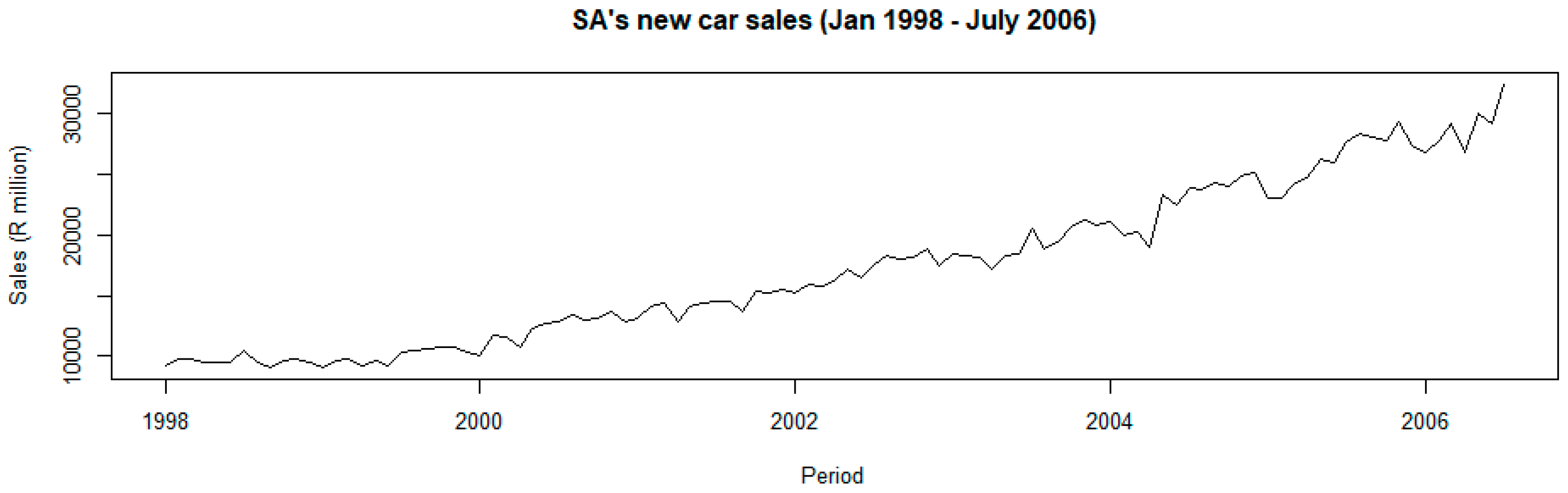
Monthly new car sales in SA average ZAR 17,281.41 million. The minimum and maximum monthly sales are ZAR 9065 million and ZAR 32,399 million, respectively. The time series plot of the original new car sales is shown in Figure 1.

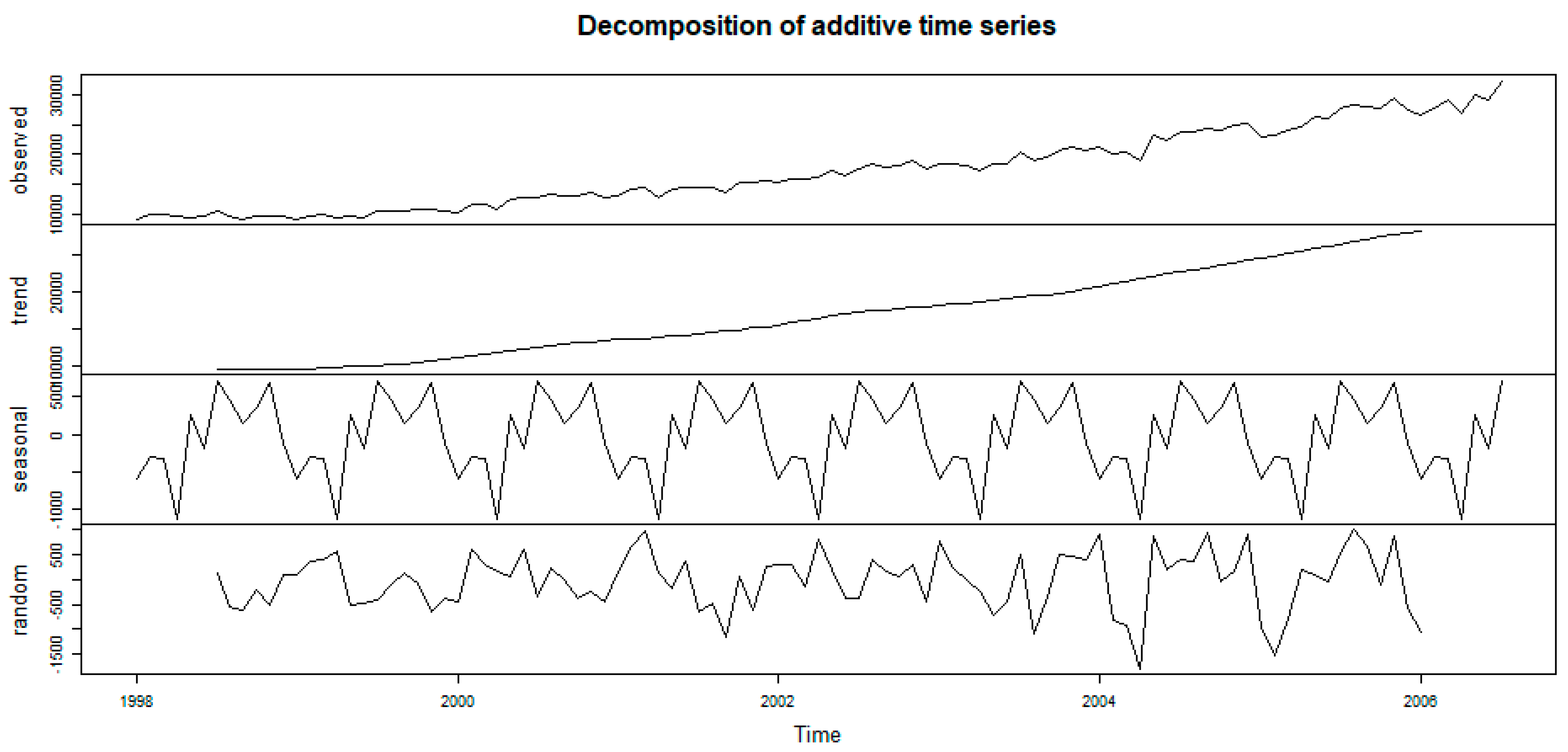
The plot shows a strong upward trend with non-constant variance, which suggests that the new car series is not stationary. Despite the growth in new car sales, the graph shows a sharp decrease in sales between 2004 and 2005. A decomposed time series is constructed to observe the major components of the data.

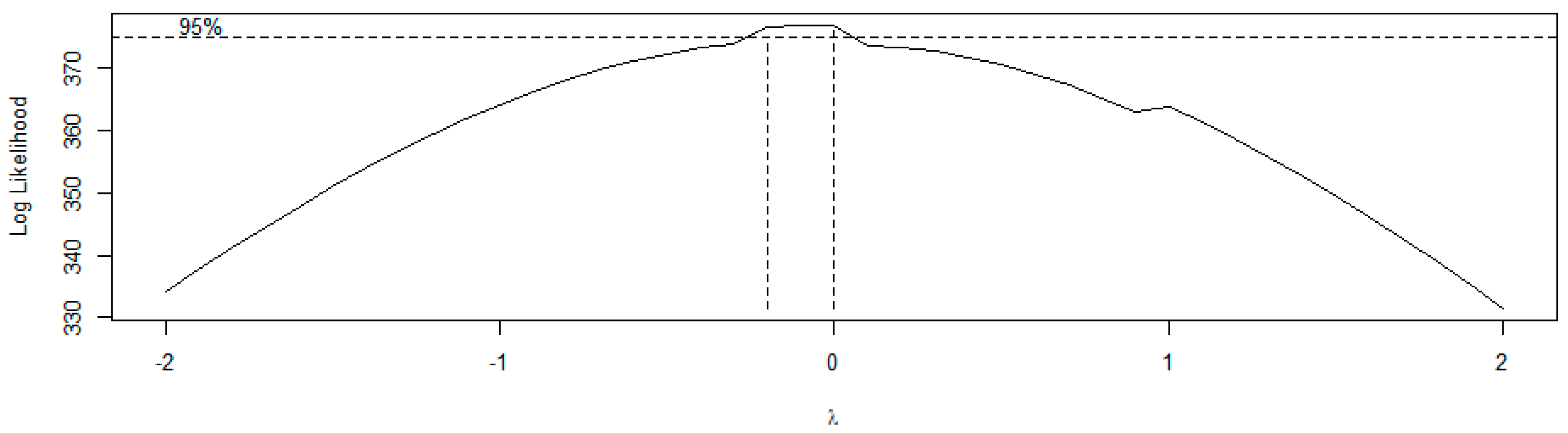
Figure 2 indicate a non-stationary series with a strong upward trend and some seasonal variation. This suggests the need for some data transformation, including differencing to achieve stationarity of the data. The Box–Cox technique is used in determining the best and appropriate data transformation to be applied.

Figure 2 shows from top to bottom the whole time series, long-term trend component, seasonality component, and the random component.

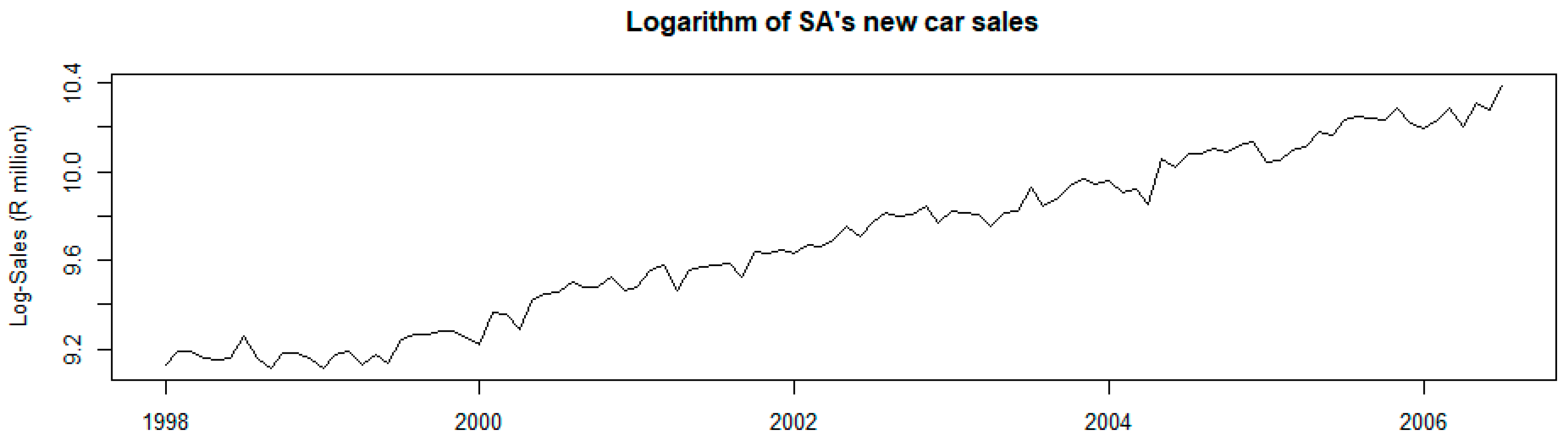
Figure 3 below shows that the maximum loglikelihood of the transformation parameter lambda $\left(\lambda \right)$ is 0. This suggests the need for a logarithm transformation to tame the variance and smooth the series. A logarithm transformation is applied to the new car sales data $\left(Y_t\right)$, and the log-transformed new car sales is denoted by $Z_t=log\left(Y_t\right).$ A plot of $Z_t$ is shown in Figure 4.

A smoother but non-stationary series is exhibited in Figure 4. An ADF test is applied to the log-transformed data to examine the stationarity of the data.

Table 2. ADF test results of log-transformed data $\left(Z_t\right)$.

Dickey–Fuller	Lag Order	p-Value
−2.2964	4	0.4538

presents the ADF test results of the log-transformed data.

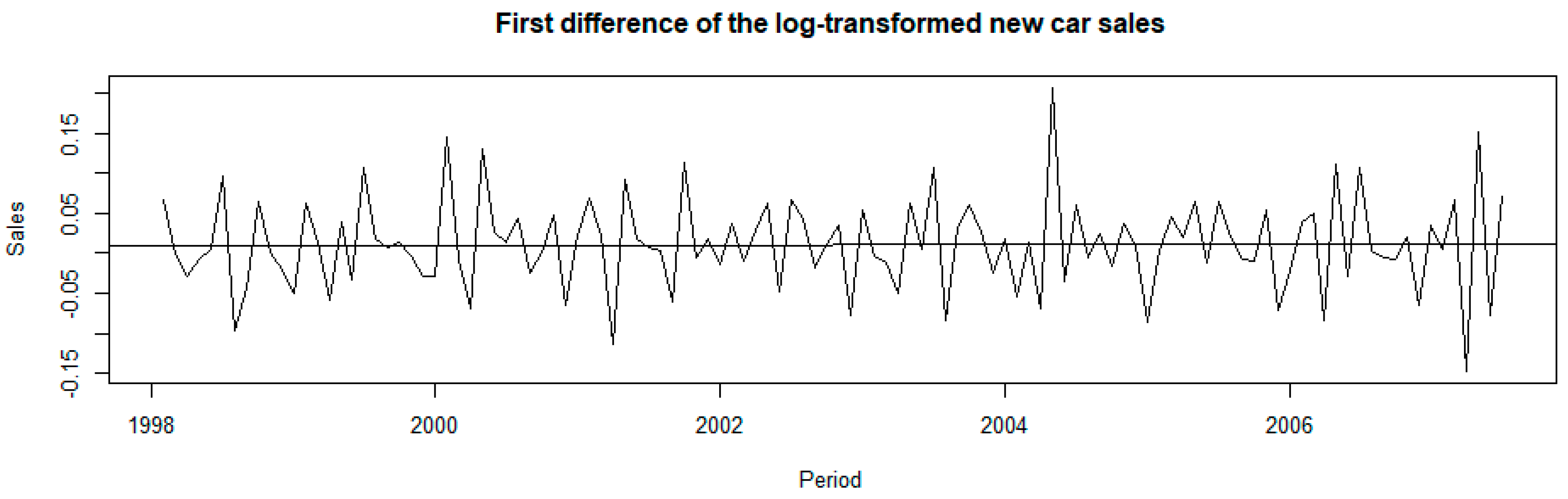
The results presented in Table 2 confirm the non-stationarity of the log-transformed motor vehicle sales data as suggested by the p-value of 0.2444; therefore, we failed to reject the null hypothesis of the presence of unit root in the data. The series is non-stationary. An ordinary first difference is applied to the log-transformed data. Figure 5 is a graphic representation of the first difference in the log-transformed motor vehicle sales.

Figure 5 depicts a stationary series; therefore, the first difference of the log-transformed new car sales shows the absence of a unit root. To further confirm this, an ADF test is employed on the first difference of the log-transformed new car sales.

Table 3. ADF test of first difference of the log-transformed new car sales.

Dickey–Fuller	Lag Order	p-Value
−5.4218	4	0.01

is a summary of the results.

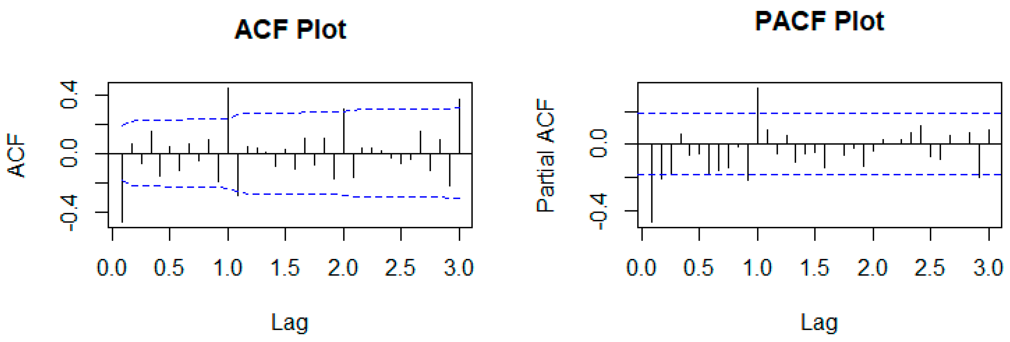
At the 5% significance level, the log-transformed new car sales data are stationary after the first ordinary difference, as evidenced by the small p-value of 0.01. Both the ACF and PACF of the first difference of the log-transformed motor vehicle sales data are conducted to visualize the appropriate $p,d$, and $q$, as well for the identification of the tentative model. Figure 6 presents the ACF and PACF plots of the first ordinary differenced log-transformed data.

In the ACF and PACF plots, the blue lines are boundary lines used to identify statistically significant ACF or PACF coefficients or lags. The ACF and PACF plots of first ordinary differenced log-transformed new car sales suggest the use of models such as the SARIMA (0,1,1)(0,0,2)₁₂ and SARIMA (0,1,1)(1,0,2)₁₂. The EACF is plotted as well to further check the proposed models. The EACF is shown in

Table 4. The EACF.

AR/MA
	0	1	2	3	4	5	6	7	8	9	10	11	12	13
0	x	o	O	o	x	o	o	o	O	o	o	x	x	o
1	o	x	O	o	o	o	o	o	O	o	o	x	o	o
2	x	x	X	o	o	o	o	o	O	o	o	x	o	o
3	x	o	O	o	o	o	o	o	O	o	o	x	o	o
4	x	o	O	o	o	o	o	o	o	o	o	x	o	o
5	x	x	X	o	o	o	o	o	o	o	o	x	x	o
6	x	x	X	o	o	o	o	o	o	o	o	x	x	o
7	x	x	X	o	o	o	o	x	o	o	o	x	x	o

.

The EACF results suggest employing a model such as SARIMA (0,1,1)(0,0,2)₁₂. The suggested model is fitted with other models, and the best model is selected with the support of the AIC and BIC.

Table 5. Fitted models’ AIC, BIC, and adequacy measures.

Model	AIC	BIC	RMSE	MAPE
SARIMA (0,1,1)(0,0,2)12 model with drift	−332.65	−319.53	0.0806	0.0003
SARIMA (0,1,1)(0,0,1)12 model with drift	−329.90	−319.40	0.0883	0.0003
SARIMA (1,1,1)(0,0,2)12 model with drift	−322.89	−309.77	0.0814	0.0006
SARIMA (1,1,0)(0,0,2)12 model with drift	−320.5	−310.00	0.0812	0.0008

Note: the final model considered is bold.

presents the fitted models together with AIC and BIC measures, as well as out-of-sample RMSE and MAPE values.

Table 5 shows that the SARIMA ${\left(\mathrm{0,1},1\right)(\mathrm{0,0},2)}_{12}$ model with drift indicates the lowest values for most of the measures considered. It is thus deemed the best model for new car sales in SA. The SARIMA (0,1,1)(0,0,2)₁₂ model is written as:

$$Z_t=Z_{t-1}+c+{\epsilon }_t+{\theta }_1{\epsilon }_{t-1}+{\mathsf{\Theta }}_1{\epsilon }_{t-12}+{\mathsf{\Theta }}_2{\epsilon }_{t-24}+{\theta }_1{\mathsf{\Theta }}_1{\epsilon }_{t-13}+{\theta }_1{\mathsf{\Theta }}_2{\epsilon }_{t-25},$$

(6)

where $c$ is the mean of the log-transformed new car sales, ${\theta }_1$ is the non-seasonal MA model parameter, and ${\mathsf{\Theta }}_1$ and ${\mathsf{\Theta }}_2$ are the seasonal MA model parameters. The SARIMA ${\left(\mathrm{0,1},1\right)(\mathrm{0,0},2)}_{12}$ model parameters are presented in

Table 6. SARIMA ${\left(\mathrm{0,1},1\right)(\mathrm{0,0},2)}_{12}$ model parameters.

Parameter	Coefficient/Parameter Estimate	Standard Error (SE)	Test Statistic	p-Value
${\theta }_1$	−0.5591	0.0871	−6.4161	<0.0001
${\mathsf{\Theta }}_1$	0.2676	0.1076	2.4859	0.0129
${\mathsf{\Theta }}_2$	0.2570	0.1214	2.1178	0.0342
C	0.0109	0.0028	3.8154	0.0001

.

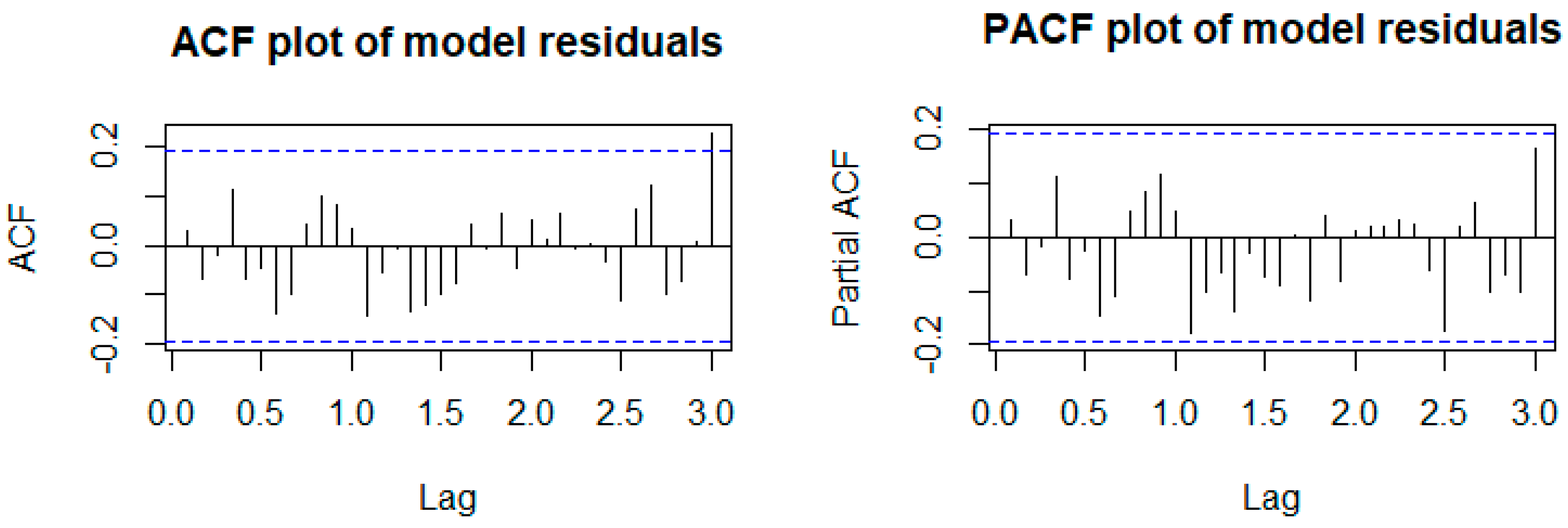
All the model parameters presented in Table 6 are statistically significant, as evidenced by large test statistics and small p-values. The ACF and PACF plots of the SARIMA ${\left(\mathrm{0,1},1\right)(\mathrm{0,0},2)}_{12}$ model residuals are shown in Figure 7.

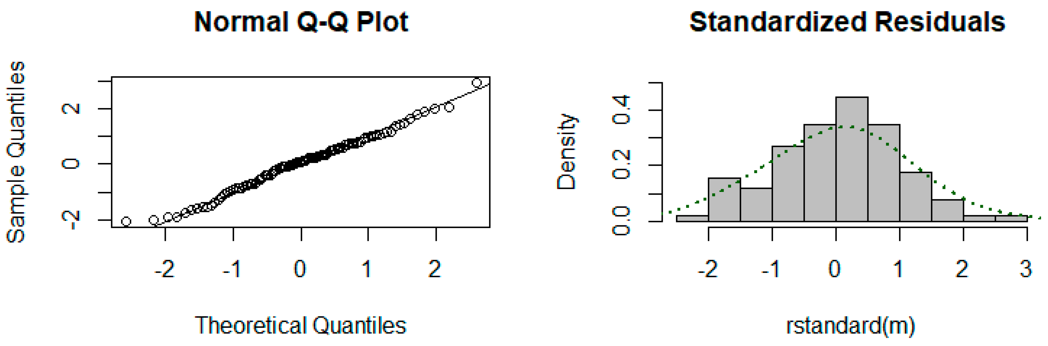
The SARIMA (0,1,1)(0,0,2)₁₂ model residuals seem to be uncorrelated. The model residuals’ Q-Q plot and histogram are constructed to check for normality. Figure 8 presents the normality plots.

The Q-Q plot and histogram of the SARIMA (0,1,1)(0,0,2)₁₂ model residuals suggest that the model residuals are indeed normally distributed. The SARIMA (0,1,1)(0,0,2)₁₂ model is confirmed to be best suited to SA’s monthly new car sales; hence, the model is used to forecast future new car sales.

4.2. In-Sample and Out-of-Sample Forecasting

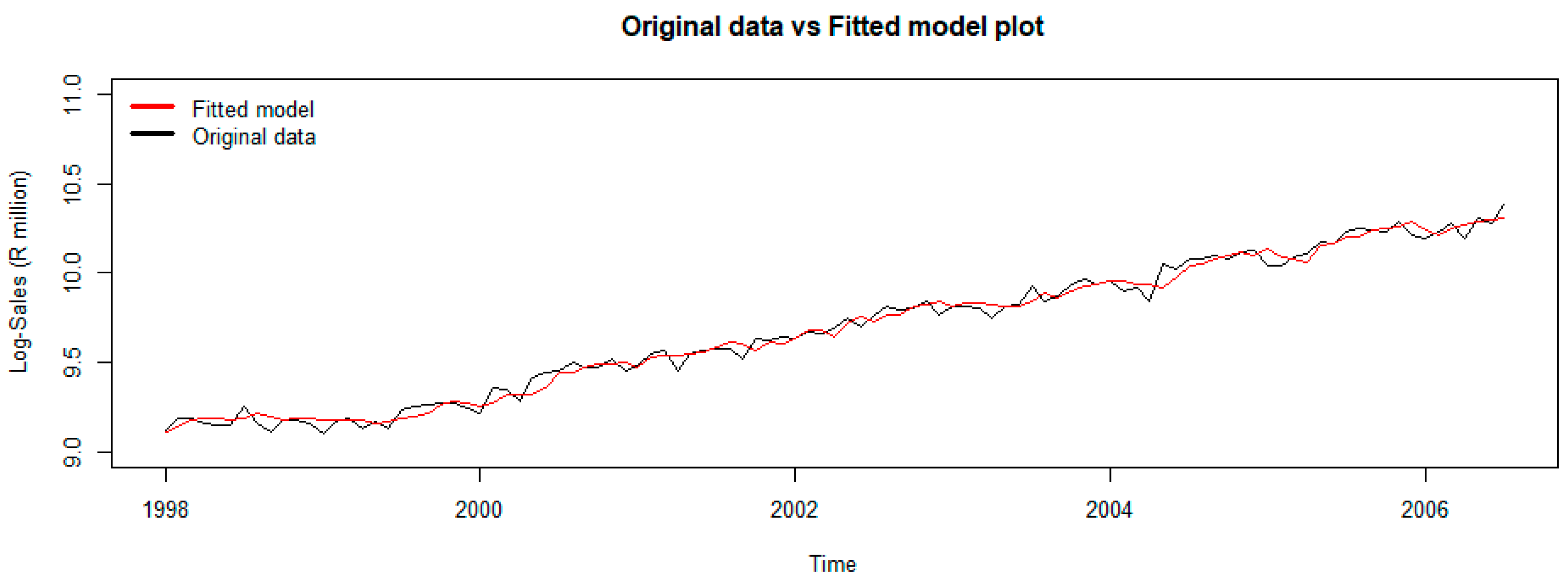
Forecasts of future new car sales for SA are important for the government’s tax purposes, as well as for all automotive industry stakeholders in terms of planning and marketing purposes and policy formulation. The SARIMA (0,1,1)(0,0,2)₁₂ model is used to generate in-sample and out-of-sample forecasts for the next 209 months. Figure 9 shows the original series versus the in-sample fitted values.

Figure 9 illustrates that the SARIMA (0,1,1)(0,0,2)₁₂ model is valid. The fitted values and the original values do not differ significantly. This suggests that the model and the data are well-matched.

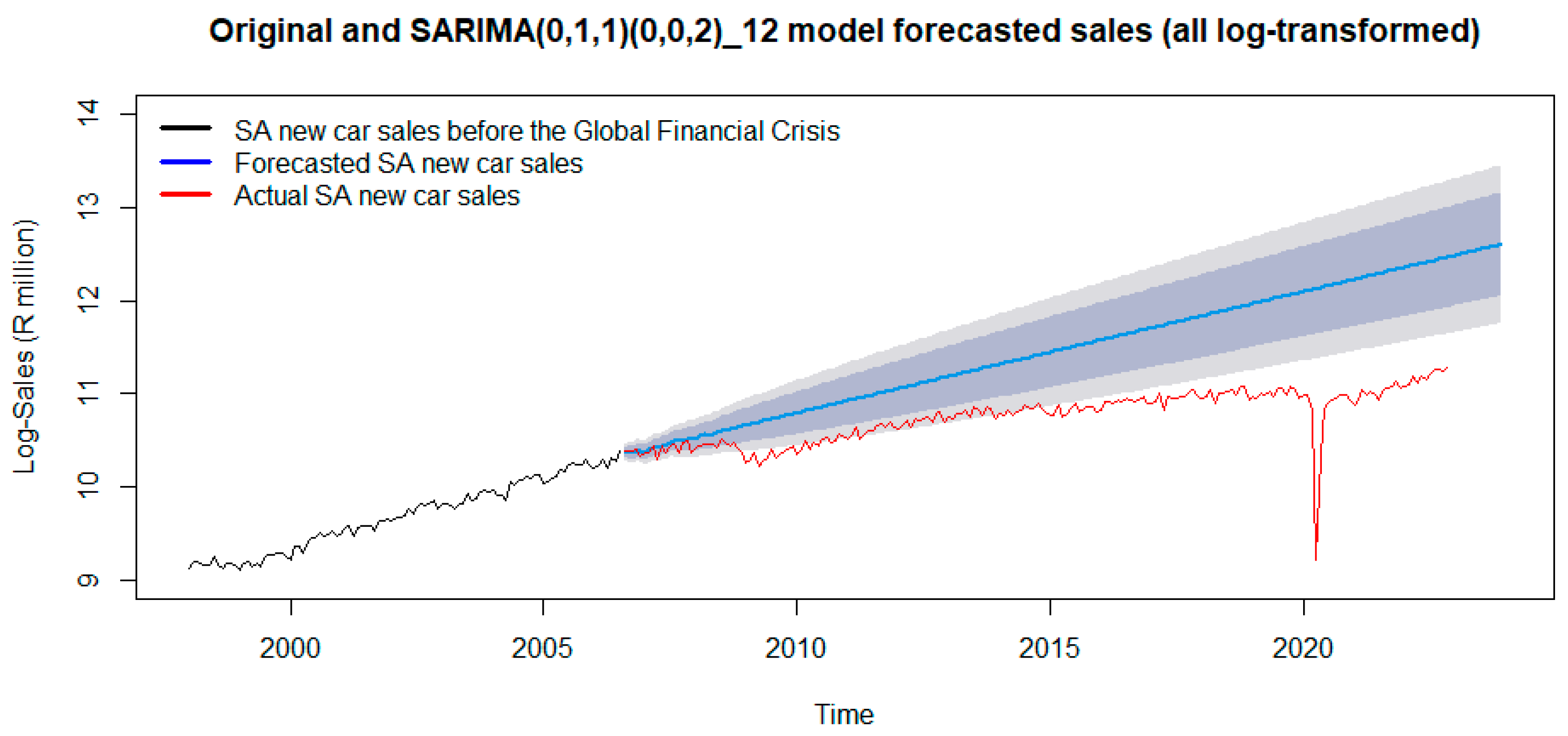
A 209-month out-of-sample forecast is made, with values compared to actual new automobile sales, covering the period from August 2006 to December 2023. The forecasts are presented in Figure 10.

Table A1. New car forecasts, actual and differences.

Month	Predicted Sales	Actual Sales	Differences	Month	Predicted Sales	Actual Sales	Differences
Aug 2006	31,716	32,486	−770	May 2015	15-May	97,484	48,708
Sep 2006	31,832	32,326	−494	Jun 2015	15-Jun	98,548	50,741
Oct 2006	31,782	32,065	−283	Jul 2015	15-Jul	99,624	53,733
Nov 2006	32,572	32,695	−123	Aug 2015	15-Aug	100,712	49,636
Dec 2006	32,411	30,675	1736	Sep 2015	15-Sep	101,811	51,222
Jan 2007	31,824	31,740	84	Oct 2015	15-Oct	102,923	51,867
Feb 2007	32,623	31,924	699	Nov 2015	15-Nov	104,046	51,759
Mar 2007	33,517	34,115	−598	Dec 2015	15-Dec	105,182	49,180
Apr 2007	33,482	29,423	4059	Jan 2016	16-Jan	106,331	49,867
May 2007	34,295	34,232	63	Feb 2016	16-Feb	107,491	54,478
Jun 2007	34,269	31,662	2607	Mar 2016	16-Mar	108,665	54,702
Jul 2007	35,706	33,992	1714	Apr 2016	16-Apr	109,851	54,355
Aug 2007	35,999	34,879	1120	May 2016	16-May	111,051	56,240
Sep 2007	36,112	31,950	4162	Jun 2016	16-Jun	112,263	54,771
Oct 2007	36,317	35,229	1088	Jul 2016	113,489	57,272	56,217
Nov 2007	37,050	35,739	1311	Aug 2016	114,728	55,606	59,122
Dec 2007	36,669	31,529	5140	Sep 2016	115,980	55,303	60,677
Jan 2008	37,023	33,381	3642	Oct 2016	117,246	56,035	61,211
Feb 2008	37,816	34,411	3405	Nov 2016	118,526	58,352	60,174
Mar 2008	38,484	34,590	3894	Dec 2016	119,820	54,316	65,504
Apr 2008	38,045	34,725	3320	Jan 2017	121,128	53,674	67,454
May 2008	39,002	34,634	4368	Feb 2017	122,451	55,299	67,152
Jun 2008	39,149	33,611	5538	Mar 2017	123,788	60,342	63,446
Jul 2008	40,449	36,996	3453	Apr 2017	125,139	50,530	74,609
Aug 2008	40,454	35,340	5114	May 2017	126,505	57,943	68,562
Sep 2008	40,896	33,979	6917	Jun 2017	127,886	56,987	70,899
Oct 2008	41,342	35,612	5730	Jul 2017	129,283	56,489	72,794
Nov 2008	41,794	33,232	8562	Aug 2017	130,694	58,110	72,584
Dec 2008	42,250	31,792	10,458	Sep 2017	132,121	57,576	74,545
Jan 2009	42,711	28,365	14,346	Oct 2017	133,563	61,135	72,428
Feb 2009	43,178	29,252	13,926	Nov 2017	135,021	62,889	72,132
Mar 2009	43,649	31,583	12,066	Dec 2017	136,495	57,515	78,980
Apr 2009	44,125	27,554	16,571	Jan 2018	137,986	57,211	80,775
May 2009	44,607	29,016	15,591	Feb 2018	139,492	57,509	81,983
Jun 2009	45,094	30,289	14,805	Mar 2018	141,015	62,936	78,079
Jul 2009	45,587	32,822	12,765	Apr 2018	142,554	53,531	89,023
Aug 2009	46,084	29,935	16,149	May 2018	144,111	60,467	83,644
Sep 2009	46,587	30,991	15,596	Jun 2018	145,684	59,603	86,081
Oct 2009	47,096	32,129	14,967	Jul 2018	147,275	60,840	86,435
Nov 2009	47,610	33,166	14,444	Aug 2018	148,882	62,122	86,760
Dec 2009	48,130	33,817	14,313	Sep 2018	150,508	58,713	91,795
Jan 2010	48,655	31,212	17,443	Oct 2018	152,151	65,150	87,001
Feb 2010	49,187	32,851	16,336	Nov 2018	153,812	65,163	88,649
Mar 2010	49,724	35,932	13,792	Dec 2018	155,491	55,523	99,968
Apr 2010	50,266	33,047	17,219	Jan 2019	157,189	58,073	99,116
May 2010	50,815	35,228	15,587	Feb 2019	158,905	56,474	102,431
Jun 2010	51,370	34,339	17,031	Mar 2019	160,640	60,017	100,623
Jul 2010	51,931	36,639	15,292	Apr 2019	162,394	59,300	103,094
Aug 2010	52,498	37,361	15,137	May 2019	164,166	61,310	102,856
Sep 2010	53,071	35,383	17,688	Jun 2019	165,959	58,510	107,449
Oct 2010	53,650	36,104	17,546	Jul 2019	167,771	63,926	103,845
Nov 2010	54,236	38,656	15,580	Aug 2019	169,602	63,025	106,577
Dec 2010	54,828	38,234	16,594	Sep 2019	171,454	58,745	112,709
Jan 2011	55,427	36,634	18,793	Oct 2019	173,326	64,669	108,657
Feb 2011	56,032	37,745	18,287	Nov 2019	175,218	62,465	112,753
Mar 2011	56,643	41,754	14,889	Dec 2019	177,131	56,859	120,272
Apr 2011	57,262	36,440	20,822	Jan 2020	179,065	58,804	120,261
May 2011	57,887	38,961	18,926	Feb 2020	181,020	59,193	121,827
Jun 2011	58,519	40,199	18,320	Mar 2020	182,996	50,282	132,714
Jul 2011	59,158	40,275	18,883	Apr 2020	184,994	9984	175,010
Aug 2011	59,804	42,306	17,498	May 2020	187,013	30,529	156,484
Sep 2011	60,457	42,951	17,506	Jun 2020	189,055	50,658	138,397
Oct 2011	61,117	41,373	19,744	Jul 2020	191,119	54,854	136,265
Nov 2011	61,784	44,273	17,511	Aug 2020	193,205	55,427	137,778
Dec 2011	62,458	41,470	20,988	Sep 2020	195,315	58,247	137,068
Jan 2012	63,140	40,655	22,485	Oct 2020	197,447	59,408	138,039
Feb 2012	63,830	42,712	21,118	Nov 2020	199,603	58,928	140,675
Mar 2012	64,526	45,275	19,251	Dec 2020	201,782	55,940	145,842
Apr 2012	65,231	41,466	23,765	Jan 2021	203,985	52,684	151,301
May 2012	65,943	45,722	20,221	Feb 2021	206,212	56,411	149,801
Jun 2012	66,663	44,620	22,043	Mar 2021	208,463	62,668	145,795
Jul 2012	67,391	45,567	21,824	Apr 2021	210,739	59,186	151,553
Aug 2012	68,126	46,476	21,650	May 2021	213,040	61,068	151,972
Sep 2012	68,870	44,368	24,502	Jun 2021	215,365	59,124	156,241
Oct 2012	69,622	48,716	20,906	Jul 2021	217,717	55,584	162,133
Nov 2012	70,382	49,240	21,142	Aug 2021	220,094	61,961	158,133
Dec 2012	71,151	43,992	27,159	Sep 2021	222,496	63,794	158,702
Jan 2013	71,927	46,613	25,314	Oct 2021	224,925	64,650	160,275
Feb 2013	72,713	45,936	26,777	Nov 2021	227,381	68,640	158,741
Mar 2013	73,506	47,922	25,584	Dec 2021	229,863	63,570	166,293
Apr 2013	74,309	47,992	26,317	Jan 2022	232,373	64,307	168,066
May 2013	75,120	49,884	25,236	Feb 2022	234,910	66,109	168,801
Jun 2013	75,940	46,508	29,432	Mar 2022	237,474	71,747	165,727
Jul 2013	76,769	51,491	25,278	Apr 2022	240,067	66,563	173,504
Aug 2013	77,608	50,521	27,087	May 2022	242,688	71,587	171,101
Sep 2013	78,455	47,449	31,006	Jun 2022	245,337	69,060	176,277
Oct 2013	79,311	51,721	27,590	Jul 2022	248,016	73,233	174,783
Nov 2013	80,177	50,689	29,488	Aug 2022	250,724	77,045	173,679
Dec 2013	81,053	46,061	34,992	Sep 2022	253,461	77,864	175,597
Jan 2014	81,937	48,487	33,450	Oct 2022	256,228	76,149	180,079
Feb 2014	82,832	47,779	35,053	Nov 2022	259,025	78,537	180,488
Mar 2014	83,736	49,783	33,953	Dec 2022	261,853
Apr 2014	84,650	47,428	37,222	Jan 2023	264,712
May-14	85,575	49,500	36,075	Feb 2023	267,602
Jun-14	86,509	49,823	36,686	Mar 2023	270,523
Jul-14	87,453	53,245	34,208	Apr 2023	273,477
Aug-14	88,408	51,309	37,099	May 2023	276,462
Sep-14	89,373	51,231	38,142	Jun 2023	279,481
Oct-14	90,349	54,108	36,241	Jul 2023	282,532
Nov-14	91,335	50,912	40,423	Aug 2023	285,616
Dec-14	92,332	48,832	43,500	Sep 2023	288,735
Jan-15	93,340	47,584	45,756	Oct 2023	291,887
Feb-15	94,360	47,442	46,918	Nov 2023	295,073
Mar-15	95,390	52,780	42,610	Dec 2023	298,295
Apr-15	96,431	46,863	49,568

in the annexure presents the actual and projected new car sales figures on the original scale after reversing the data transformations.

An increase in future new motor sales, after the GFC, is predicted. The disparity between the blue line (forecasted expected future new car sales had the GFC not occurred) and the red line (actual new car sales) reflects the impact of the GFC on the automotive industry’s new car sales. By July 2010, the sales had recovered to their pre-GFC levels, but not enough for the original sales trajectory to be maintained. Though the rate of increase in car sales somewhat recovered, the level remained stubbornly low. The rate of increase in car sales needs to increase further in order to attain the original trajectory. The COVID-19 pandemic (2020) further hampered the situation, as a sharp decrease was experienced. The noticeable steep decline at the beginning of 2020 suggests that the COVID-19 pandemic had an even greater impact on new car sales. Therefore, it will take some time for the sales to stabilize around the expected trajectory had the GFC and the pandemic not occurred. SA’s economy has been deprived of the maximum benefits that could have been provided by its automobile industry. To ensure that the automotive sector produces the necessary amount of goods and services, policies could be put in place to jumpstart the industry.

5. Discussion

This study evaluated and predicted the enduring effects of the GFC on new car sales in SA by using currently available empirical data. The results and conclusions have been derived through the application of standard statistical validation techniques to the fitted model. The analysis indicates new car sales in SA exhibit periodic fluctuations and seasonality, with higher sales being registered during certain months, such as December. The fitted model results show a positive outlook for future new car sales in SA; however, the SA automotive industry has been negatively affected by the GFC and is still to fully recover from its lingering effects. These findings align with previous research conducted by [38], who determined that the GFC had a detrimental effect on the automobile industry in the USA. Specifically, the authors identified a decline in car manufacturing company sales due to the prevailing market situation and the economic slump. Further, [10] similarly found that the GFC shock negatively affected the USA’s prominent automotive industry, as well as several other sectors of the American economy.

Rena and Msoni [4,39,40] arrived at similar conclusions regarding the negative impact of the GFC on the SA economy. The GFC resulted in the loss of almost a million jobs in 2009 alone, causing the real unemployment rate to rise to 32%. Moreover, the demand for SA products, including new cars, was marked by a significant decline due to reduced global demand ([39,40]). The private sector also suffered, as the GFC led to a substantial reduction in available credit, resulting in a sharp fall in the services sector, such as construction and automobiles, as highlighted by [40]. These findings indicate the severity of the GFC’s effect on SA’s economy, including the car manufacturing industry. This finding is echoed by [41], whose study suggests that the delay in the purchase of high-value items, such as new cars, by consumers, resulted in decreased income for large automotive firms.

The results of the aforementioned studies suggest that it will take time for the industry to fully recover from the GFC’s lingering negative effects to catch up to the expected trend line. Further, the findings indicate that the impact of external economic shocks, such as the GFC, can have long-lasting effects on the industry and undermine the ability to achieve sustainable growth. Policymakers and industry stakeholders could take this into account when developing strategies to promote the recovery and growth of the sector, including measures for mitigating the effects of external economic shocks and promoting innovation and competitiveness in the industry. The industry can become more resilient and better equipped to weather future economic challenges and disruptions, ensuring its continued contribution to SA’s economy, through information/data-led decisions. While the GFC devastated new car sales in SA, projected estimates suggest that new car sales will increase in the coming years as economic conditions keep improving.

6. Conclusions

This paper investigates how the GFC affected the sale of new cars in SA. A quantitative method (the Box–Jenkins technique) was chosen as the method of analysis because it can effectively capture important characteristics, such as long-term trends and seasonality in new car sales, while also providing more precise projections. A clear, increasing, uninterrupted trend in the new car sales series is evident. Actual post-GFC car sales show an increase, going forward, at about the same rate as before the GFC, but from a lower base. The lower rate of increase in future new car sales in SA addresses this paper’s research question regarding current and future new car sales. The study hypothesizes that the GFC has had a negative long-term impact on new car sales in SA.

The latter affects economic growth in SA since new car sales are often seen as an indicator of consumer confidence and economic growth. The increase, albeit at a lower rate, can help to stimulate SA’s economic growth and create jobs in the automotive industry and related sectors. The expected slower growth suggests an increasing demand for vehicles, which can lead to improved production and sales for automakers and dealerships. This will positively influence the supply chain for new car sales, as manufacturers and suppliers can increase production to meet the evidently increasing demand. Since increased demand for new cars can also drive innovation and improvements in technology, the latter could be evidenced in the automotive industry; automakers can work to differentiate their products and stay ahead of competitors. Consequently, new features and capabilities in vehicles, as well as improvements in vehicles’ fuel efficiency and environmental performance, may be expected.

It is interesting to note that, despite the concerted efforts of SA’s government and policymakers to restore stability, the 2007/2008 GFC resulted in a major reduction in new car sales, which contributed to the economy’s decline. Currently, new car sales have not reached the numbers expected in the absence of the GFC. This study’s findings confirm the hypothesis that the GFC had a significant and negative long-term impact on new car sales in SA. Given the potential for the automotive industry to generate employment and economic growth, it may be prudent for policymakers to focus on supporting the manufacturing and selling of new vehicles in the country as a way of growing the economy. By doing so, SA could benefit from increased economic activity, especially from neighboring countries, and improved earnings in this sector.

Saliently, while the study’s findings suggest a negative long-term impact of the GFC on new car sales in SA, the limitations of the SARIMA model used in the analysis may limit the generalizability of the results to other African countries. Factors such as the size and structure of the automotive industry, as well as the broader economic and social context, can vary significantly between countries. This may influence the GFC’s effect on new car sales in different ways. With its state-of-the-art car assemblies, SA is the dominant economic powerhouse in southern Africa. Many countries in the region import new cars from mainly South Africa and from second-hand markets in other countries, such as Japan.

Nonetheless, the research holds importance as the inferences derived from it could potentially be valuable within the South African setting and in neighboring countries.

7. Recommendations

Industrial policies expressly aimed at the automotive sector are needed to boost car sales to their expected levels. The government may help automakers by offering incentives to export more of their goods to other nations. SA may have lost some of its market to competitors, and such incentives are needed to regain those markets. New car sales generate more income, raising the GDP, tax, and living standards of a nation.