Datasets of Groundwater Level and Surface Water Budget in a Central Mediterranean Site (21 June 2017–1 October 2022)

Abstract

This note makes available five years of data gathered in a measurement site equipped with a micrometeorological station and two monitoring wells. Series of data of hydrological and atmospheric variables make it possible to estimate the flux of water across the atmosphere-land interface and to calculate the water budget, which are crucial topics in climate and environmental sciences. The water-table measures began during 2017, one of the driest years of the whole instrumental period of climate history for the Central Mediterranean. Data from the micrometeorological station have been used to construct two more datasets of daily and monthly totals of different terms of the surface water budget, from which the net infiltration has been estimated. An apparent decreasing trend characterizes both the data time series of groundwater level and estimated infiltration in the considered period.

Data Set: The datasets are stored on the Zenodo repository: https://doi.org/10.5281/zenodo.7572140.

Data Set License: CC-BY 4.0

1. Summary

Datasets including groundwater level, soil moisture, and meteorological variables make it possible to estimate fluxes of water and energy across the atmosphere–land interface and to calculate water budgets [1,2,3,4,5]. Given their fundamental importance in climate and environmental sciences, series of data of hydrological and atmospheric variables taken at specific sites are becoming increasingly freely shared [6,7,8].

Several regions in the world, including the Euro-Mediterranean, were affected by declining groundwater resources in recent decades [9,10]. Drought events linked to increases of temperature, in combination with decreasing precipitation in the summer months, have been indicated among the main causes [11,12]. From July 2016 to June 2017 western-central Europe was affected by the most severe meteorological drought at the continental scale since at least 1979 [13]. Winter 2016/17 was drier than normal in the Central Mediterranean, with precipitation totals reaching only 60% of normal precipitation [14]. In 2017, Italy experienced the driest year of the whole instrumental period of its climate history [15].

Since June 2017, the Institute of Atmospheric Sciences and Climate of the National Research Council of Italy (ISAC-CNR) has taken measures of water-table depth of a shallow karst aquifer (the Miocene Aquifer of Central-Eastern Salento, hereinafter referred as MACES) located in the Salento Peninsula (Apulia region, Italy). The measures are taken from two wells located several hundred meters from the ISAC-CNR Micrometeorological Station (IMS), which has been in operation since June 2002 [16,17,18]. As a whole, wells and station constitute a measurement site that allows direct comparison between hydrological and weather data. Due to their climate sensitivity and subsurface heterogeneity, the karst systems located in dry lands require particular attention when it comes to processing data related to the exchanges between air, soil and groundwater [19,20]. Series of data from this site have been used to interpret the local water consumption during the lockdown for COVID-19 [21]. Datasets of IMS were previously used to calculate recharge time and specific yield of the regional deep aquifer [22,23]. This note provides and makes available five hydrological years (from 1 October to 30 September in the Northern Hemisphere) of gathered data with the aim of promoting open science and fostering cooperation by making related descriptions and insights shareable.

2. Data Descriptor

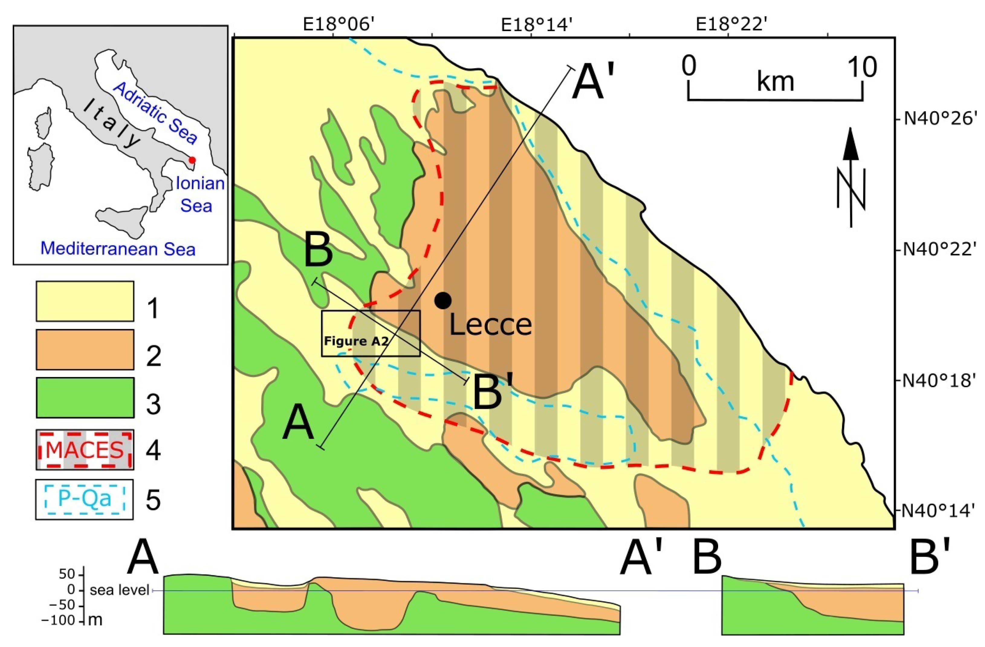
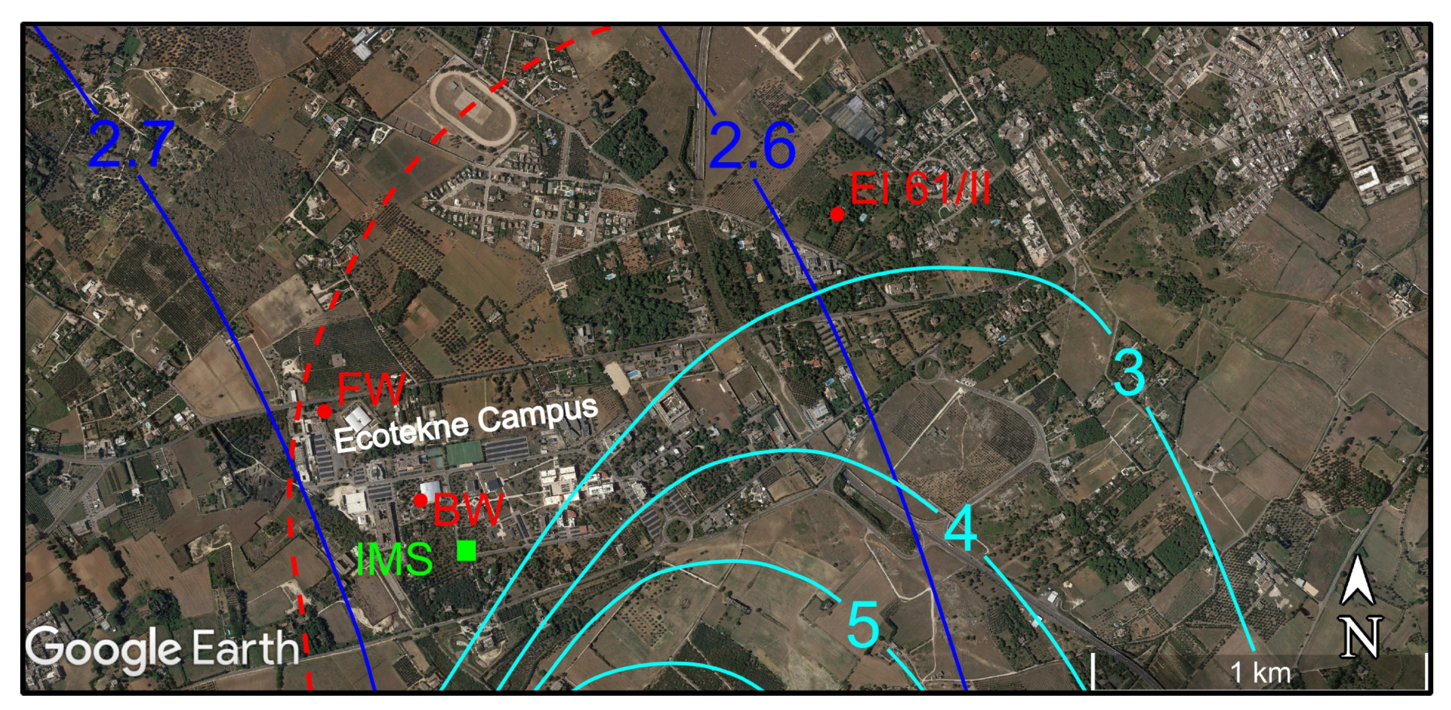
2.1. Geophysical Setting

Located in the Central Mediterranean, the Salento Peninsula constitutes a lowland plateau (maximum altitude 200 m) surrounded by the Ionian Sea to the West and South and by the Adriatic Sea to the East. Annual precipitations are usually between 600 and 700 mm and less than Italian average because of the low orography and the residual blocking effect of the Apennine Chain (150 km NW of Salento), for the incoming cyclonic moisture flux coming from the Atlantic Ocean, generally accompanied by southerly winds. Moderate northerly winds typically blow during the daytime in high pressure conditions, with clear skies and strong insolation. The warm/dry season (April–September) is characterized by temperatures that can reach 40 °C and more, and reduced precipitations, while the cold/wet season (October–March) by mild autumn–winter temperatures (generally above zero even at night) and enhanced precipitation. In recent years, there has been a generalized tendency to an increase in more intense, brief precipitation events during the spring–summer months [22].

Groundwater resources of the Salento Peninsula are contained in a complex system of aquifers, consisting of a main regional reservoir, the Cretaceous Aquifer (CA), and several shallow aquifers [24,25,26]. Among these latter, MACES is the most important in terms of stored groundwater volume. It is supplied by meteoric water and two Plio-Quaternary aquifers, and extensively exploited for irrigation and domestic purposes through several licensed and unlicensed wells. In the warm/dry season, MACES is recharged by irrigation water withdrawn from the CA (more hydrogeological features are given in Appendix A).

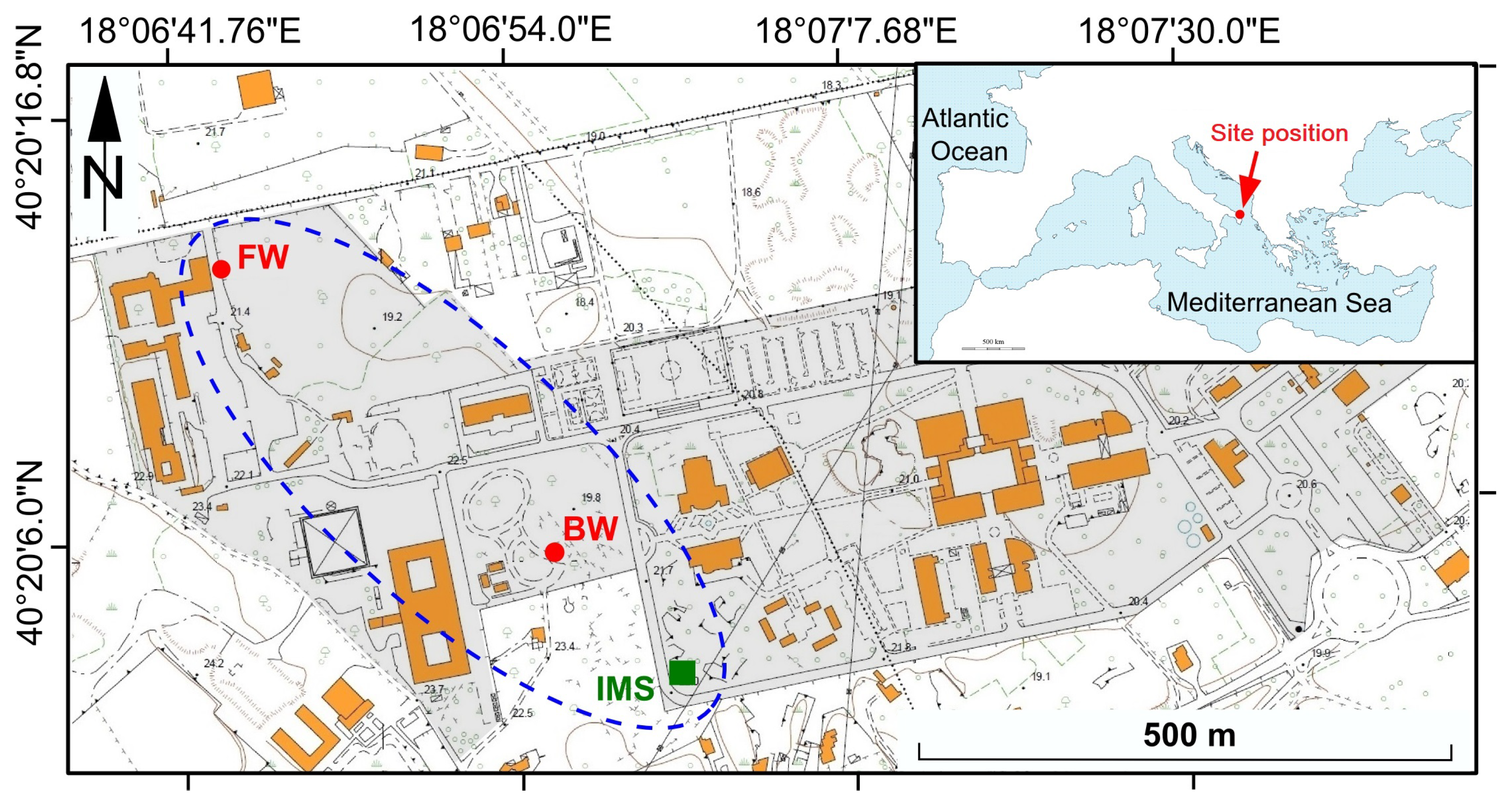
2.2. Site and Surface Data

The measurement site is placed in a suburban area 5 km south-west from Lecce (Figure A1), within the Ecotekne Campus of the University of Salento, with mixed local vegetation including Mediterranean shrubs, pines and olive groves, scattered buildings, and quarried surfaces (Figure 1). Here, the MACES water table lies at a depth of 20–22 m below the ground, in good agreement with literature data [21,27].

The IMS [16,17] has been a data provider for the Hymex (Hydrological Mediterranean Experiment) project’s long term campaign [28]. It is mainly devoted to water and energy surface–atmosphere transfer, and is composed of two complementary systems, collecting data based on half-hour averages: (1) a 16 m height mast equipped with a fast response eddy covariance system and basic meteorological data; (2) a micrometeorological station that also collects standard meteorological and soil surface data in a dedicated data logger. The mast has a typical flux footprint fetch in the order of hundreds of meters [22,29], thus taking contributions from the campus and some immediately surrounding vegetated areas. Both data files from the two systems are stored in local memory and then transferred to the web data base once per day through UMTS connection system [18]. The collected data of precipitation, real evapotranspiration, and soil moisture also allow the estimation of the net infiltration as described in Section 3, together with more details about measurements and sensors.

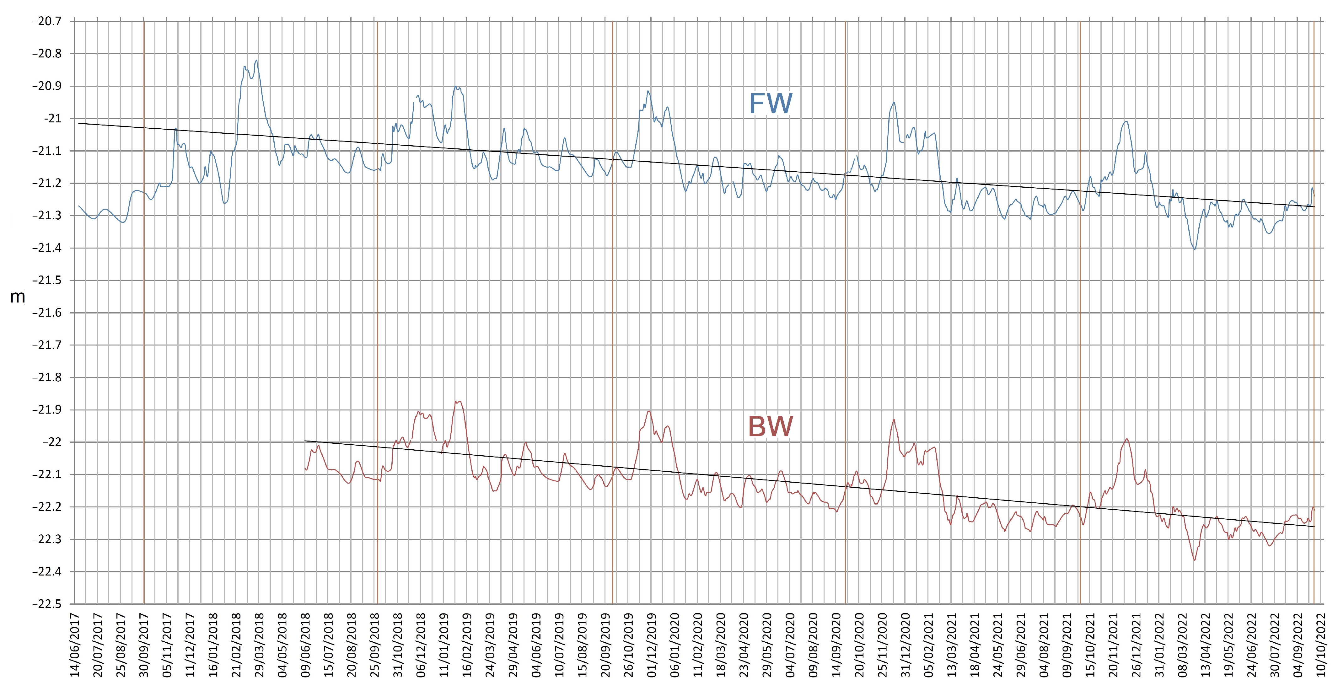
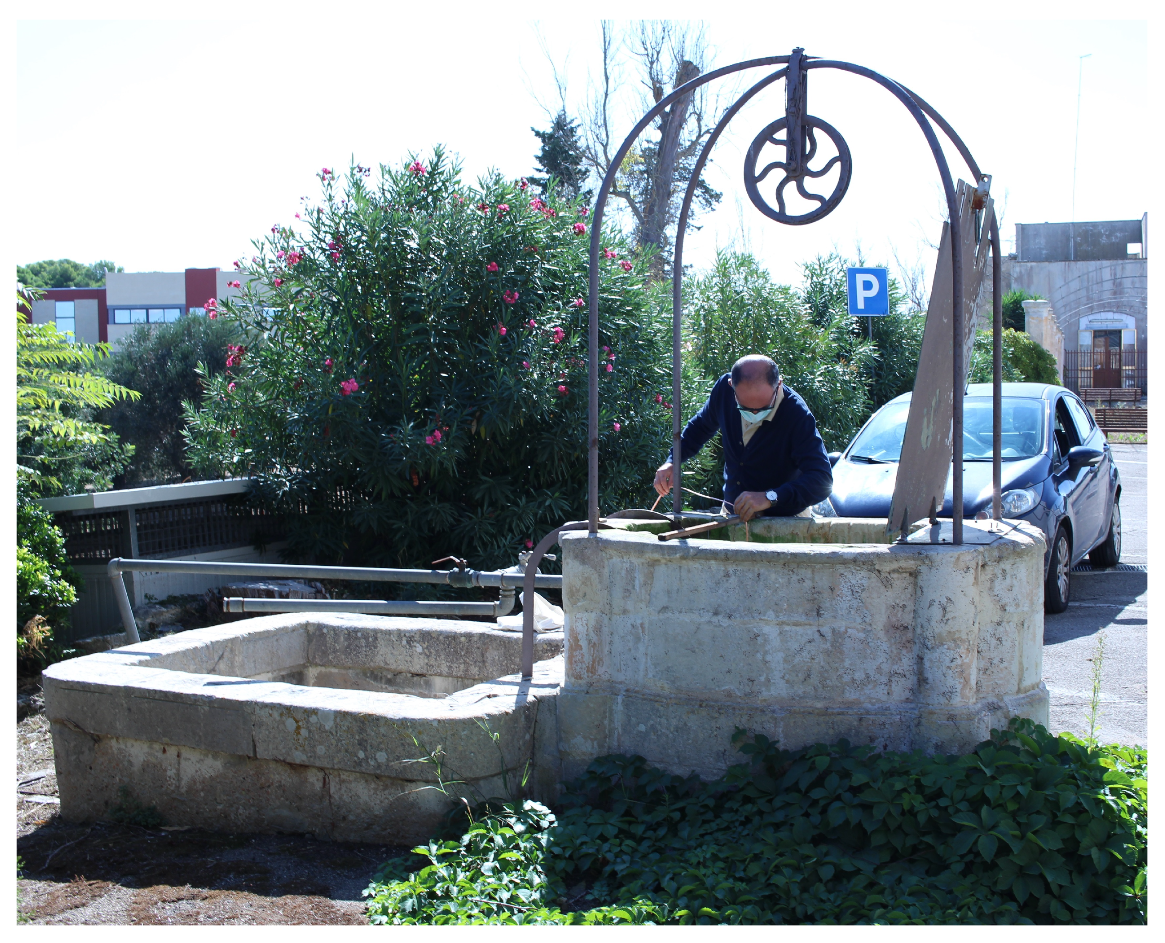
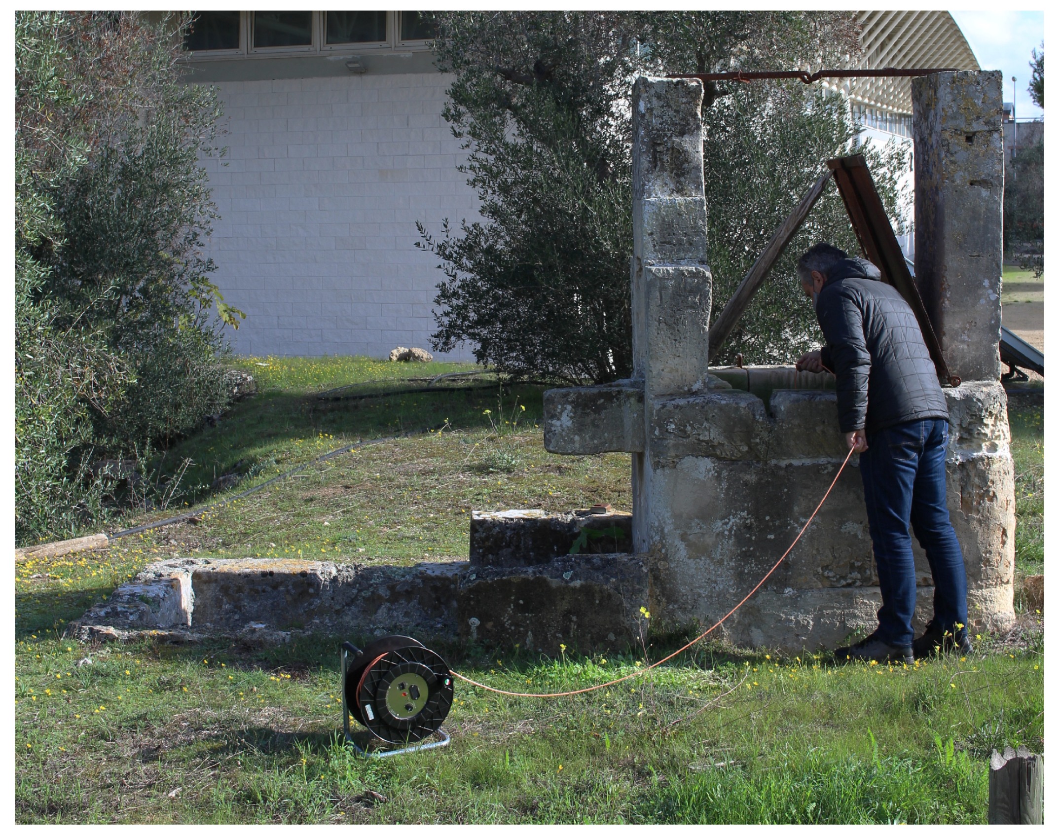
2.3. Groundwater Level Data (Manual Measurements)

The two monitoring wells of the measurement site (named Fiorini, FW, and Benessere, BW, Figure 1) were hand dug about 25 m deep one century ago, to provide water for agriculture and rural settlements. The wells are easily identifiable by their stone well heads (Figure A3 and Figure A4). Based on the provincial technical map at a scale of 1:5000, the height of the well head is 22.5 for FW and 24.7 m a.s.l. for BW. Google Earth geographic coordinates are: 40°20′11.93″ N, 18°06′43.09″ E, for FW; 40°20′03.50″ N, 18°06′55.30″ E, for BW.

Manual measurements of groundwater levels (as water-table depth below the well head, see Figure A5) began in June 2017 for FW, and in June 2018 for BW. They have been taken using a portable electronic water-table meter (Boviar GST-FR100), with an average frequency of one measure about every three days for both wells (for more details see Appendix B). The frequency of measurement was established during the first months of the monitoring aiming to obtain relatively detailed well hydrographs. However, during some rainy events, the measurements were made more frequently in order to better document the rise in the groundwater level. Despite the laboriousness of the field operations, the use of a water-table meter makes it possible to overcome problems related to the lack of research funding and the reliability of measurements in cases of equipment malfunction [30,31,32]. Well hydrographs contain valuable information on aquifer responses to both natural and human stresses [33].

2.4. Data Records

The dataset of the water-table depths taken from 21 June 2017 to 1 October 2022 is supplied as a text file in the Zenodo repository (see “S1.txt” in https://zenodo.org/record/7572140). The columns represent the following items:

- date (dd/mm/yy)

- water-table depth measured in FW (m)

- water-table depth measured in BW (m).

There are a few gaps in the dataset, because sometimes adverse weather conditions prevented measurement for one of the two wells. The curves of the variations of the groundwater head in the monitored wells are shown in Figure 2.

For FW, the measure of the water-table depth started in the middle of the warm/dry season (June 2017) of the 2016–2017 hydrological year. A year later (June 2018), monitoring of BW began. Note that the two lines fit almost perfectly. Only in very few cases were the daily variations in FW and BW of the opposite sign (see “S1.txt” in https://zenodo.org/record/7572140). A general negative trend from the hydrological year 2017–2018 to 2021–2022 is apparent. At the end of the 2021–2022 hydrological year (June-September 2022), the groundwater level in FW was nearly coincident with that of June–September 2017.

The surface water budget datasets are available in the Zenodo repository (see “S2.txt” and “S3.txt” in https://zenodo.org/record/7572140) as text files of daily/monthly data. The columns represent the following items:

- date (Julian day or fraction of year representing the end of each month)

- precipitation (daily/monthly total, m)

- real evapotranspiration (daily/monthly total, m)

- soil moisture 2 cm (beginning of the day/month, m³/m³)

- soil moisture 2 cm (end of the day/month, m³/m³)

- soil moisture 35 cm (beginning of the day/month, m³/m³)

- soil moisture 35 cm (end of the day/month, m³/m³)

- estimated net infiltration (daily/monthly total, m)

- percentage of validated data (daily/monthly total)

- corrected real evapotranspiration (daily/monthly total corrected by percentage of validated data, m)

- corrected net infiltration (daily/monthly total corrected by percentage of validated data, m).

The corrected monthly net infiltration values for the MACES are shown in Figure 3, where still possible negative values have been set to zero to properly represent the groundwater contribution (see also Section 3). Other data are plotted in Figure A6 and Figure A7 (Appendix C).

3. Methods

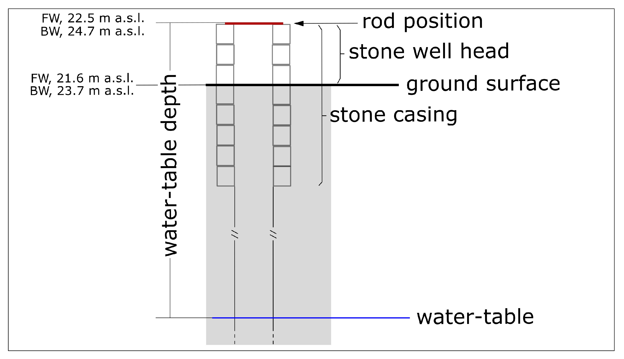
3.1. Groundwater Level Measurements

To collect groundwater levels data, reference points were fixed on the stone casing of each monitored well. A rod was placed on the well head to reference the depth read by the water-table meter (Appendix B, Figure A3 and Figure A5). In this way, it was possible to measure the depth with an accuracy of 0.5 cm. Furthermore, this system allowed the use of several operators without affecting the reliability of the data.

3.2. Surface Measurements

3.2.1. Telescopic Mast (Top Level 14 m above Surface)

The Eddy covariance system (measurements of turbulence, heat, and evapotranspiration fluxes) is composed by one Solent–Gill 20 Hz ultrasonic anemometer and one Campbell Kh20 Krypton hygrometer. One thermohygrometer allows standard air temperature and humidity measurements (Rotronic MP100). Data are firstly collected in a dedicated notebook that calculates the half hour eddy covariance statistics rotated in the ‘streamline’ coordinate system [34] before storage in a daily data file.

3.2.2. Micrometeorological Station

It is equipped with standard meteorological sensors and soil data sensors (data are collected by a dedicated Campbel CR1000-X datalogger).

Standard sensors (2 m height):

Cup anemometer (Campbell A100R), windvane (Campbell W200P), thermohygrometer (Rotronic MP100), four-components net radiometer (Hukseflux NR01), precipitation gauge (EM ARG100), pressure sensor (Campbell PTB101B).

Soil sensors:

2 thermistor temperature sensors (Campbell109L, 2 and 5 cm depth), 2 thermopile soil heat flux sensors (Hukseflux HFP01, 2 and 5 cm depth), 2 moisture content capacitive sensors (Decagon EC-5, 2 and 35 cm depth).

A selection of the available IMS data can be visualized at the address [18] in graphic format. Data are freely available upon request at the address indicated in the staff area. Part of the dataset is also available in the Hymex site for subscribed users [35].

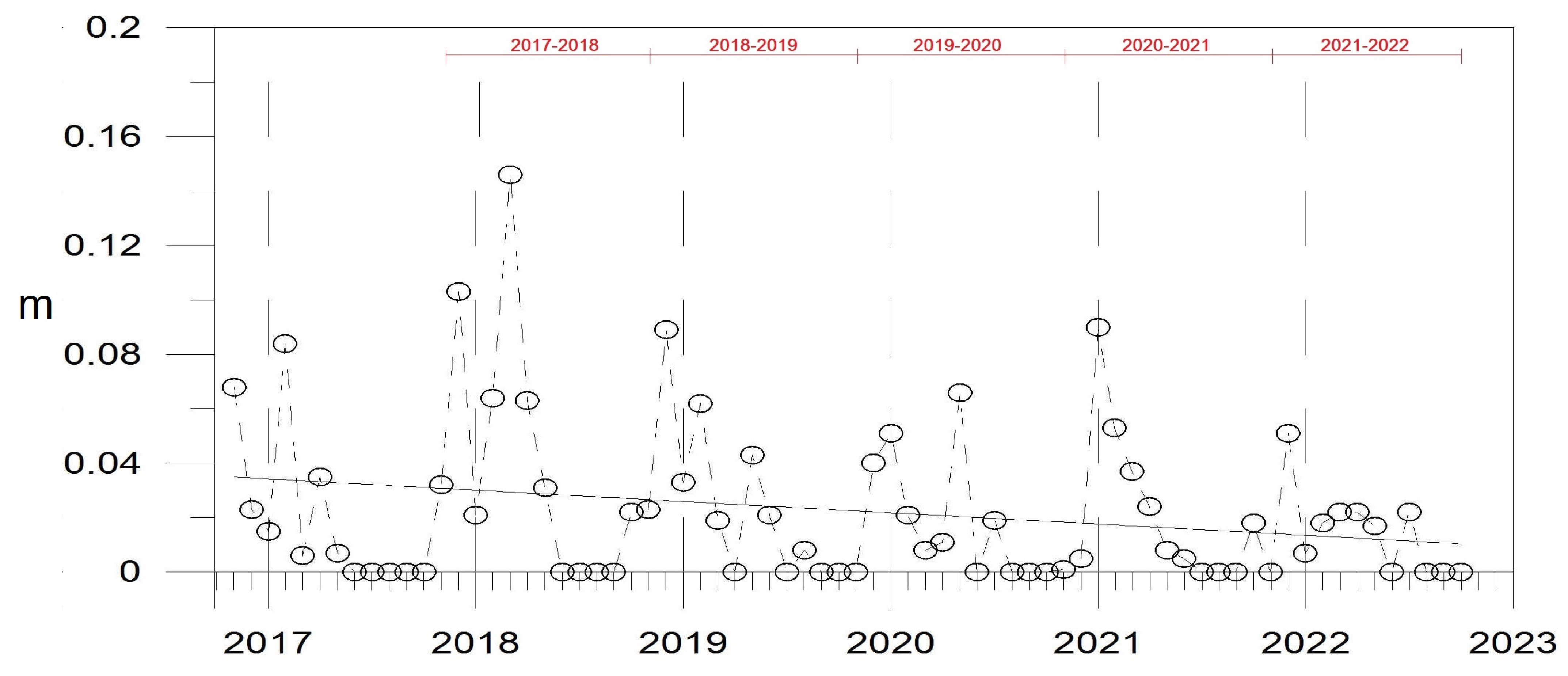
3.3. Surface Water Budget

For the surface water budget, in order to estimate the net infiltration, the following mass conservation equation is considered [22,36,37]:

$$S(t+dt)=S\left(t\right)+P-E-I-R+Ir,$$

(1)

where $S\left(t\right)$ is the soil water content per unit area, and P, E, I, R, and Ir are the total precipitation, actual evapotranspiration, net infiltration, surface-subsurface runoff, and irrigation water in the time interval dt, respectively. Due to the hydrological features of the measurement site and its surroundings, the runoff term R has been neglected. In fact, the site is placed on a large sub-horizontal ground without any appreciable slope, thus neither stream systems nor persistent pond waters are present.

To quantify the surface water transfer data from the IMS the following data have been used:

(1) total precipitation P;

(2) averaged evapotranspiration flux;

(3) averaged soil moisture at 2 cm (s1) and 35 cm (s2) depth.

All data are taken on a 30 min base interval (averages, and totals for precipitation). The averaged evapotranspiration flux has then been transformed to 30-minutes total evapotranspiration E.

After calculating the total daily/monthly values for the above quantities, the daily/ monthly net infiltration I has been calculated by the following expression between the initial $\left(t\right)$ and final $(t+dt)$ time of each day/month [22]:

$$I=P-E-S(t+dt)+S\left(t\right),$$

(2)

In Equation (2) the Ir term has been neglected (as well as R). The anthropic irrigation is indeed absent in the measurement area but still present over the whole MACES region and will be the object of further studies. In Equation (2) P and E are directly derived by the measurements, while $S\left(t\right)$ has been calculated approximating an average soil moisture content per square meter as:

$$S\left(t\right)=h\left(s1\right(t)+s2(t\left)\right)/2,$$

(3)

where s1 and s2 are the available soil moisture density measurements (in m³/m³ at 2 cm and 35 cm underground, respectively) and h represents an effective soil thickness estimated as approximately 0.4 m [22]. Negative values of I (Equation (2)) are still possible in very dry conditions because of the approximations in Equation (3) but they must also be considered, as vanishing contributes to the MACES water balance (see also [22]). In the daily/monthly averaging of the evapotranspiration, where it is more likely to have some missing data, the actual percentage of the available data has also been calculated, generally resulting in over 80%. The results have then been corrected, adding the product of the lacking data percentage times of the calculated daily/monthly average to each total value, to approximately compensate for the effect of the missing data. The estimated infiltration for MACES is shown in Figure 3 with the related linear trend. A more complete data view can be found in “S2.txt” and “S3.txt” in Zenodo repository (https://zenodo.org/record/7572140).

4. User Notes

The trend of the water-table fluctuations (Figure 2) apparently suggests a decline of the groundwater resource and is in agreement with the negative trend in the estimated infiltration for the considered five hydrological years (Figure 3). The infiltration decrease is associated with a decrease in precipitation in the considered five years, while the real evapotranspiration shows a less significant negative trend in the same period (see also Appendix C). Thus, the reduced surface water input affects the MACES groundwater input. This finding gives an insight into the natural stresses that affected MACES from 2017 to 2022. However, no data are available regarding the shallow groundwater exploitation for domestic and irrigation uses [21]. Moreover, the recharge of MACES by irrigation water (Ir) withdrawn from the CA during the warm/dry season is unknown. This currently prevents the calculation of the actual aquifer water budget. The measurements in the site herein shown and the sharing of the updated datasets are scheduled to continue for several more years.

References

1. Van Lanen, H.A.J.; Peters, E. Definition, Effects and Assessment of Groundwater Droughts. In Drought and Drought Mitigation in Europe; Vogt, J.V., Somma, F., Eds.; Springer: Dordrecht, The Netherlands, 2000; Volume 14, pp. 49–61. [Google Scholar]
2. Reghunath, R.; Murthy, T.R.S.; Raghavan, B.R. Time Series Analysis to Monitor and Assess Water Resources: A Moving Average Approach. Environ. Monit. Assess. 2005, 109, 65–72. [Google Scholar] [CrossRef] [PubMed]
3. Van der Velde, Y.; de Rooij, G.H.; Torfs, P.J.J.F. Catchment-scale non-linear groundwater-surface water interactions in densely drained lowland catchments. Hydrol. Earth Syst. Sci. 2009, 13, 1867–1885. [Google Scholar] [CrossRef]
4. Cerlini, P.; Meniconi, S.; Brunone, B. Groundwater Supply and Climate Change Management by Means of Global Atmospheric Datasets. Preliminary Results. Procedia Eng. 2017, 186C, 420–427. [Google Scholar] [CrossRef]
5. Varadharajan, C.; Agarwal, D.A.; Brown, W.; Burrus, M.; Carroll, R.W.H.; Christianson, D.S.; Dafflon, B.; Dwivedi, D.; Enquist, B.J.; Faybishenko, B.; et al. Challenges in Building an End-to-End System for Acquisition, Management, and Integration of Diverse Data From Sensor Networks in Watersheds: Lessons From a Mountainous Community Observatory in East River, Colorado. IEEE Access 2019, 7, 182796–182813. [Google Scholar] [CrossRef]
6. Zabala, M.E.; Sanchez-Murillo, R.; Dietrich, S.; Gorocito, M.; Vives, L.; Manzano, M.; Varni, M. Hydrological dataset of a sub-humid continental plain basin (Buenos Aires, Argentina). Data Br. 2020, 33, 106400. [Google Scholar] [CrossRef]
7. Nordio, G.; Fagherazzi, S. Groundwater, soil moisture, light and weather data collected in a coastal forest bordering a salt marsh in the Delmarva Peninsula (VA). Data Br. 2022, 45, 108584. [Google Scholar] [CrossRef]
8. Taufik, M.; Marliana, T.W.; Awaluddin, A.; Mukharomah, A.K.; Minasny, B. Groundwater table and soil-hydrological properties datasets of Indonesian peatlands. Data Br. 2022, 41, 107903. [Google Scholar] [CrossRef]
9. Lancia, M.; Petitta, M.; Zheng, C.; Saroli, M. Hydrogeological insights and modelling for sustainable use of a stressed carbonate aquifer in the Mediterranean area: From passive withdrawals to active management. J. Hydrol. Reg. Stud. 2020, 32, 100749. [Google Scholar] [CrossRef]
10. Xanke, J.; Liesch, T. Quantification and possible causes of declining groundwater resources in the Euro-Mediterranean region from 2003 to 2020. Hydrogeol. J. 2022, 30, 379–400. [Google Scholar] [CrossRef]
11. Hanel, M.; Rakovec, O.; Markonis, Y.; Maca, P.; Samaniego, L.; Kyselý, J.; Kumar, R. Revisiting the recent European droughts from a long-term perspective. Sci. Rep. 2018, 8, 9499. [Google Scholar] [CrossRef] [Green Version]
12. Moravec, V.; Markonis, Y.; Rakovec, O.; Svoboda, M.; Trnka, M.; Kumar, R.; Hanel, M. Europe under multi-year droughts: How severe was the 2014–2018 drought period? Environ. Res. Lett. 2021, 16, 034062. [Google Scholar] [CrossRef]
13. Garcia-Herrera, R.; Garrido-Perez, J.M.; Barriopedro, D.; Ordonez, C.; Vicente-Serrano, S.M.; Nieto, R.; Gimeno, L.; Sorí, R.; Yiou, P. The European 2016/17 Drought. J. Clim. 2019, 32, 3169–3187. [Google Scholar] [CrossRef]
14. Bissolli, P.; Demircan, M.; Kennedy, J.J.; Lakatos, M.; McCarthy, M.; Morice, C.; Pastor Saavedra, S.; Pons, M.R.; Rodriguez Camino, C.; Rösner, B.; et al. Europe and the Middle East. In State of the Climate in 2017. Special Supplement of the Bulletin of the American Meteorological Society; Blunden, J., Arndt, D.S., Hartfield, G., Eds.; American Meteorological Society: Boston, MA, USA, 2018; pp. 222–232. [Google Scholar]
15. 2017 Dryest Year in Italy for 200 Years. Available online: https://www.ansa.it/english/news/science_tecnology/2017/12/04/2017-dryest-year-in-italy-for-200-years-4_79d13a9e-d0fc-461f-a0c4-36ee4fa33cdb.html (accessed on 10 November 2022).
16. Martano, P.; Elefante, C.; Grasso, F. A Database for long-term atmosphere-surface transfer monitoring in Salento peninsula (Southern Italy). Dataset Pap. Sci. 2013, 2013, 946431. [Google Scholar] [CrossRef]
17. Martano, P.; Elefante, C.; Grasso, F. Ten years water and energy surface balance from the CNR-ISAC micrometeorological station in Salento peninsula (Southern Italy). Adv. Sci. Res. 2015, 12, 121–125. [Google Scholar] [CrossRef]
18. ISAC-CNR. Micrometeorological Station. Available online: http://www.basesperimentale.le.isac.cnr.it (accessed on 10 December 2022).
19. Hartmann, A.; Gleeson, T.; Wada, Y.; Wagener, T. Enhanced groundwater recharge rates and altered recharge sensitivity to climate variability through subsurface heterogeneity. Proc. Natl. Acad. Sci. USA 2017, 114, 2842–2847. [Google Scholar] [CrossRef]
20. Berthelin, R.; Rinderer, M.; Andreo, B.; Baker, A.; Kilian, D.; Leonhardt, G.; Lotz, A.; Lichtenwoehrer, K.; Mudarra, M.; Padilla, I.Y.; et al. A soil moisture monitoring network to characterize karstic recharge and evapotranspiration at five representative sites across the globe. Geosci. Instrum. Method. Data Syst. 2020, 9, 11–23. [Google Scholar] [CrossRef]
21. Alfio, M.R.; Balacco, G.; Delle Rose, M.; Fidelibus, C.; Martano, P. A Hydrometeorological Study of Groundwater Level Changes during the COVID-19 Lockdown Year (Salento Peninsula, Italy). Sustainability 2022, 14, 1710. [Google Scholar] [CrossRef]
22. Delle Rose, M.; Martano, P. Infiltration and Short-Time Recharge in Deep Karst Aquifer of the Salento Peninsula (Southern Italy): An Observational Study. Water 2018, 10, 260. [Google Scholar] [CrossRef]
23. Delle Rose, M.; Fidelibus, C.; Martano, P. Assessment of Specific Yield in Karstified Fractured Rock through the Water-Budget Method. Geosciences 2018, 8, 344. [Google Scholar] [CrossRef]
24. Tadolini, T.; Tazioli, G.S.; Tulipano, L. Hydrogeology of the Idume springs area (Lecce). Geol. Appl. Idrogeol. 1971, 4, 41–63. (In Italian) [Google Scholar]
25. Tadolini, T.; Tulipano, L. The evolution of fresh-water/salt-water equilibrium in connection with withd rawals from the coastal carbonate and carstic aquifer of the Salentine Peninsula (Southern Italy). Geol. Jaharb. 1981, 29, 69–85. [Google Scholar]
26. Delle Rose, M. Sedimentological features of the Plio-Quaternary aquifers of Salento (Puglia). In Memorie Descrittive della Carta Geologica d’Italia; Istituto Superiore per la Protezione e la Ricerca Ambientale: Rome, Italy, 2007; Volume 76, pp. 137–145. [Google Scholar]
27. Tadolini, T.; Calo, G.; Spizzico, M.; Tinelli, R. Hydrogeological characterisation of post-cretaceous soils in the San Cesario di Lecce area (Puglia). In Proceedings of the V Congresso Internazionale sulle Acque Sotterranee, Taormina, Italy, 17–21 November 1985; p. 11. (In Italian). [Google Scholar]
28. HyMeX in Brief. Available online: www.hymex.org (accessed on 30 November 2022).
29. Hsieh, C.I.; Katul, G.; Chi, T. An approximate analytical model for footprint estimation of scalar fluxes in thermally stratified atmospheric flows. Adv. Water Resour. 2000, 23, 765–772. [Google Scholar] [CrossRef]
30. Korus, J. Combining Hydraulic Head Analysis with Airborne Electromagnetics to Detect and Map Impermeable Aquifer Boundaries. Water 2018, 10, 975. [Google Scholar] [CrossRef]
31. Gorgoglione, A.; Castro, A.; Chreties, C.; Etcheverry, L. Overcoming Data Scarcity in Earth Science. Data 2020, 5, 5. [Google Scholar] [CrossRef]
32. Rochford, L.M.; Ordens, C.M.; Bulovic, N.; McIntyre, N. Voluntary metering of rural groundwater extractions: Understanding and resolving the challenges. Hydrogeol. J. 2022, 30, 2251–2266. [Google Scholar] [CrossRef]
33. Butler, J.J.; Knobbe, S.; Reboulet, E.C.; Whittemore, D.O.; Wilson, B.B.; Bohling, G.C. Water Well Hydrographs: An Underutilized Resource for Characterizing Subsurface Conditions. Groundwater 2021, 59, 808–818. [Google Scholar] [CrossRef]
34. McMillen, R. An eddy correlation Technique with extended applicability to non-simple terrain. Bound.-Layer Meteorol. 1988, 43, 231–245. [Google Scholar] [CrossRef]
35. HyMeX Database. Available online: www.hymex.org/database/ (accessed on 30 November 2022).
36. Portoghese, I.; Uricchio, V.; Vurro, M. A GIS tool for hydrogeological water balance evaluation on a regional scale in semi-arid environments. Comput. Geosci. 2005, 31, 15–27. [Google Scholar] [CrossRef]
37. Gomez, D.G.; Ochoa, C.G.; Godwin, D.; Tomasek, A.A.; Zamora Re, M.I. Soil Water Balance and Shallow Aquifer Recharge in an Irrigated Pasture Field with Clay Soils in the Willamette Valley, Oregon, USA. Hydrology 2022, 9, 60. [Google Scholar] [CrossRef]
38. Vacher, H.L. Dupuit-Ghyben-Herzberg analysis of strip-island lenses. GSA Bull. 1988, 100, 580–591. [Google Scholar] [CrossRef]
39. Delle Rose, M.; Federico, A.; Fidelibus, C. A computer simulation of groundwater salinization risk in Salento peninsula (Italy). In Proceedings of the Risk Analysis II—Second International Conference on Computer Simulation in Risk Analysis and Hazard Mitigation, Bologna, Italy, 11–13 October 2000; Brebbia, C.A., Ed.; WIT Press: Southampton, UK, 2000; pp. 465–475. [Google Scholar]
Figure 1. Map of the measurement site (topography from Lecce Province Technical Map at a scale of 1:5000). IMS, ISAC-CNR Micrometeorological Station; FW, Fiorini Well; BW, Benessere Well. Ecotekne Campus in gray (Apulia region, Italy).
Data 08 00038 g001
Figure 2. Smoothed well hydrographs with linear regression (water-table depth in meters below the well head; see Figure A5). Hydrological years are delimited; FW, Fiorini Well; BW, Benessere Well.
Data 08 00038 g002
Figure 3. Estimated monthly net infiltration in meters with linear regression (continuous line). The dashed line is intended only to help viewing. The considered hydrological years are delimited in the upper side.
Data 08 00038 g003
Disclaimer/Publisher’s Note: The statements, opinions and data contained in all publications are solely those of the individual author(s) and contributor(s) and not of MDPI and/or the editor(s). MDPI and/or the editor(s) disclaim responsibility for any injury to people or property resulting from any ideas, methods, instructions or products referred to in the content.