Data Descriptor

A Global Multiscale SPEI Dataset under an Ensemble Approach

1
Division on Impacts on Agriculture, Forests and Ecosystem Services (IAFES), Fondazione Centro Euro-Mediterraneo sui Cambiamenti Climatici (CMCC), 01100 Viterbo, Italy
2
Division on Advanced Scientific Computing (ASC), Fondazione Centro Euro-Mediterraneo sui Cambiamenti Climatici (CMCC), 73100 Lecce, Italy
3
European Commission-Joint Research Centre (JRC), 21027 Ispra, Italy
*
Author to whom correspondence should be addressed.
Submission received: 6 October 2022 / Revised: 30 January 2023 / Accepted: 2 February 2023 / Published: 5 February 2023
(This article belongs to the Section Spatial Data Science and Digital Earth)

Abstract

:
A new multiscale Standardized Precipitation Evapotranspiration Index (SPEI) dataset is provided for a reference period (1960–1999) and two future time horizons (2040–2079) and (2060–2099). The historical forcing is based on combined climate observations and reanalysis (WATer and global CHange Forcing Dataset), and the future projections are fed by the Fast Track experiment of the Inter-Sectoral Impact Model Intercomparison Project under representative concentration pathways (RCPs) 4.5 and 8.5 and by an additional Earth system model (CMCC-CESM) forced by RCP 8.5. To calculate the potential evapotranspiration (PET) input to the SPEI, the Hargreaves–Samani and Thornthwaite equations were adopted. This ensemble considers uncertainty due to different climate models, development pathways, and input formulations. The SPEI is provided for accumulation periods of potential moisture deficit from 1 to 18 months starting in each month of the year, with a focus on the within-period variability, excluding long-term warming effects on PET. In addition to supporting drought analyses, this dataset is also useful for assessing wetter-than-normal conditions spanning one or more months. The SPEI was calculated using the SPEIbase package.
Dataset:https://doi.org/10.25424/cmcc-mfd5-t060 (accessed on 3 February 2023).
Dataset License: The dataset is made available under license CC-BY.

1. Summary

The recent Sixth Assessment Report from Working Group I of the Intergovernmental Panel on Climate Change (IPCC-AR6 [1]) defines drought as a period with below-average moisture conditions, resulting in negative impacts on various components of both natural systems and socioeconomic sectors.
Many authors, e.g., Wilhite and Glantz [2] and Mishra and Singh [3], have identified four macro categories of drought: meteorological (precipitation deficits), agricultural/ecological (soil moisture deficits causing crop and plant stress), hydrological (water shortages in surface or subsurface water bodies), and socioeconomic (water supply–demand imbalance, also known as water scarcity). The distinction of drought types is neither easy nor absolute, as droughts can propagate from one type to another; therefore, there is not a universal definition of drought because, owing to their multifaceted aspects, droughts can be measured or assessed based on a single variable or through a unique index [4,5]. Slette et al. [6] analyzed 564 drought studies and found that in a surprising percentage of studies (more than 30%) drought is considered a synonym for dry conditions without assessment and/or contextualization how such dry conditions compare to normal conditions. Instead, it is crucial to adopt standardized indices that quantify a drought and flag its severity using threshold-based classifications according to the level of deviation from the norm. Not only drought severity matters, as drier-than-normal conditions are often characterized by their spatial and temporal attributes, such as extent, frequency, duration, and timing (i.e., drought onset and/or cessation period), creating specific and “novel” definitions (e.g., mega droughts, flash droughts, and snow droughts) [7].
Many indices have been developed in recent decades for drought characterization. In the case of agricultural and ecological drought assessment, the latest IPCC-AR6 selected two such indices that represent combined air, soil, and vegetation processes: the Palmer Drought Severity Index (PDSI [8]) and the Standardized Precipitation Evapotranspiration Index (SPEI [9]). Both of these indices also consider evaporative losses—and thus temperature data—which alter water availability. Using the SPEI and PDSI, Cook et al. [10] showed that increased evaporative loss due to warming not only intensifies drying dynamics in areas where there has already been a reduction in rainfall but also leads to drought in some areas predicted to dry out slightly or even be wet if only precipitation trends were considered. Moreover, considering SPEI- and PDSI-based studies, IPCC-AR6 [1] mentions a medium confidence in the observed increase in agricultural and ecological droughts on all continents, as well as both high confidence and likelihood that with global warming in the range of +1.5 °C to +4 °C, the land areas affected by increasing drought frequency and severity will expand due to decreasing precipitation and increasing atmospheric evaporative demand. Whereas the PDSI lacks multiscale character and better suited for long droughts, the SPEI is more often used to quantify deviations from normal potential soil moisture conditions (deficit or surplus) by combining thermal and humidity regimes for different accumulation periods (one or more months) and timing (onset/cessation). Although similar to the well-known Standardized Precipitation Index (SPI) [11], a multiscale indicator suitable for meteorological drought assessments, the SPEI merges monthly series of precipitation (P, mm) and potential evapotranspiration (PET, mm) rather than using P alone; therefore, it indirectly considers temperature, as well as other meteorological variables, depending on how PET is calculated. In practice, the SPEI combines the characteristics of the SPI (multiscale) and PDSI (sensitive to PET).
While drought assessment for the historical period is mainly a function of observed climate data and selected indicators [12], projections of future droughts strongly depend on the greenhouse gas concentration scenario, the time horizon, and the set of analyzed climate simulations [13].
To complement the multiscale datasets developed at global and regional scales for historical and future periods [14,15,16,17,18,19], a new SPEI dataset for accumulation periods from 1 to 18 months ending in each month of the year was first generated for a reference historical period (1960–1999) based on a combination of observed climate and reanalysis data (WATer and global CHange Forcing Dataset, (WFD)). Then, future SPEI was calculated according to an ensemble of bias-corrected projections from multiple models and two representative concentration pathways (RCP 4.5 and RCP 8.5) for two time horizons (2040–2079 and 2060–2099) produced by the Inter-Sectoral Impact Model Intercomparison Project (ISIMIP [20]) and its Fast Track (FT) experiment. Moreover, an additional Earth system model (CMCC-CESM) similar to those involved in ISIMIP-FT was considered to rely on bias-corrected data under the RCP 8.5. Whereas using the ensemble allows for consideration of the variability across simulations due to the physics of different models and the uncertain future development pathways [21], this new dataset is associated with three other peculiarities: two PET equations (Hargreaves–Samani vs. Thornthwaite) were adopted to consider the advantages, drawbacks, and uncertainty of simplified empirical formulations based on temperature supported by a wide array of literature in terms of validation and bias-correction procedures [22,23]; the multiscale aspect spanning very short (1 month) to very long (18 months) droughts; and finally, the focus on the variability within each climatological period, excluding long-term warming effects on PET. Although the presented dataset presented herein was conceived for drought analysis, the SPEI is also useful to assess wetter-than-normal conditions spanning one or more months. Table 1 shows a comparison of the characteristics of existing SPEI datasets with different spatial and temporal coverage, confirming that the dataset presented herein is valuable for the provision of high-spatial-resolution maps over medium- to long-term future horizons (in line with other global gridded datasets), in particular because it provides an ensemble comprising various components—multiple driving bias-corrected climate simulations, RCPs, and PET formulations—in addition to covering the highest number of SPEI scales among datasets covering historical-to-future time horizons.
As an example of the provided information, Figure 1 shows maps of the long-term SPEI (over 12 months) according to the two PET equations for periods characterized by very strong El Niño (November 1997–October 1998) and strong La Niña (January 1999–December 1999), highlighting the differing distribution of wetter-than-normal and drier-than-normal regions across the globe for the two opposite events. Whereas the Hargreaves–Samani formulation seems to reveal wider drier-than-normal zones under both La Niña and El Niño, the two equations agree in depicting drier conditions over the south-eastern side of sub-Saharan Africa and South America, across the south of the United States, and along Europe–Asia borders during La Niña and over central Africa, central Asia, the Amazon, and across southeast Asia during El Niño.
As an additional example, Figure 2 represents the change in the frequency (number of occurrences) of moderate-to-extreme abnormal moisture conditions (see Section 2.2) with a length of three months (SPEI-03) as the median between PET formulations for the historical period and among PET formulations, RCPs, and GCMs/ESMs for the two future periods.
Finally, Table 2 offers a view of changes in the global mean of SPEI-03 averaged along all possible timings, under the different PET formulations and as ESMs/GCMs ensemble mean under the different RCPs and time horizons. In all future scenarios, SPEI-03 is expected to be lower than the historical periods (especially under RCP8.5 and in the long term) for up to 28% and 36% under Hargreaves–Samani and Thornthwaite formulations, respectively.

2. Methods and Data Description

2.1. Input Data

For the present work, daily time series of temperature and precipitation available from the Water and Global Change (WATCH) forcing dataset (WFD) [24,25] (https://rda.ucar.edu/datasets/ds314.1/ (accessed on 3 February 2023)) were exploited. The WFD is a twentieth-century meteorological dataset based on the European Centre for Medium-Range Weather Forecasts (ECMWF) reanalysis (ERA-40 [26]) interpolated to a 0.5° by 0.5° grid with successive elevation-based correction of surface meteorological variables plus monthly bias correction mostly based on the monthly gridded observations of the Climatic Research Unit (CRU) (corrected temperature, diurnal temperature range, cloud cover, number of wet days) and the Global Precipitation Climatology Center (precipitation) [24,27]. In accordance with this dataset, the years from 1960 to 1999 were considered as a reference period.
For the future time frame, daily time series of precipitation and temperature are available thanks to the coordinated climate model simulation experiments in the frame of the Coupled Model Intercomparison Project phase 5 (CMIP5) [28]. These simulations are forced by multiple representative concentration pathways (RCPs [29]) formulated to support the IPCC AR5. However, raw climate model simulations are affected by biases that need to be reduced for the purposes of impact studies [30]. To achieve this, the ISIMIP Fast Track (FT) initiative (https://www.isimip.org/about/#simulation-rounds (accessed on 3 February 2023)) provides bias-corrected daily time series of temperature and precipitation up to 2100 that are globally downscaled (through bilinear interpolation) at a 0.5° grid resolution for five general circulation models (GCMs) and Earth system models (ESMs) participating in CMIP5: GFDL-ESM2M, HadGEM2-ES, IPSL-CM5A-LR, MIROC-ESM-CHEM, and NorESM1-M. Bias correction is based on a trend-preserving method [31] developed to adjust the probability distribution over the reference period of 1960–1999 while maintaining the climate sensitivities of the GCMs/ESMs and representing their trend and the long-term mean.
For the purpose of this work, this method was applied also to the Earth system model (ESM) developed and used by the Foundation Euro-Mediterranean Center on Climate Change (CMCC-CESM [32,33]), the raw data of which are available in the CMIP5 data archive (https://esgf-node.llnl.gov/search/cmip5/ (accessed on 3 February 2023)). For the five different ESMs already bias-corrected within the ISIMIP-FT initiative, the RCP4.5 [34] and the RCP8.5 [35] were selected, whereas projections under the RCP8.5 are available from CMCC-CESM runs. Details of the six GCMs/ESMs are shown in Table 3.

2.2. Drought Indicator

The climate variability in terms of combined thermal and moisture conditions was computed through a well-known drought indicator, the Standardized Precipitation Evapotranspiration Index (SPEI [9]), which represents interacting air, soil, and vegetation processes and thus four different attributes of agricultural and ecological droughts. The first attribute is the duration, which is defined as the balance precipitation minus potential evapotranspiration (P-PET), serving as the basis of the SPEI and representative of the potential soil moisture; it can be calculated for one or several consecutive months, namely “accumulation periods”. The second attribute is the magnitude; given a climatological reference period, the SPEI quantifies how much the potential soil moisture deviates from the norm for each month or consecutive months in the period, standardizing the values for each month and location using log–logistic distributions and classifying them as normally, moderately, severely, or extremely dry/wet (Table 4). The third attribute is the timing; the duration can be assumed to start (or end) in any month of the year, representing drought onset (or cessation). The final attribute is the frequency; over the climatological period, the number of occurrences of each magnitude class can be calculated for a considered duration and for any onset (or cessation) month. Finally, the intensity can be estimated by dividing the magnitude by duration.
The PET input to the SPEI was computed by exploiting the Hargreaves–Samani [36] and Thornthwaite [37] formulation (see Supplementary Materials) to balance the drawbacks of each in different global regions [38,39] while maintaining the simplicity of the number of input data required and reinforced by the fact that bias-correction procedures have a large supporting literature for temperature and precipitation. To disentangle the global warming effect on evapotranspiration and concentrate on interannual variability, detrending was applied directly to the monthly P minus PET time series, as in [39,40,41,42,43,44,45,46,47], rather than to the single P and PET time series in order to avoid losing physical consistency between the two variables.
The SPEI was calculated for each land cell of the WFD grid with values available for all regions (except Antarctica). All the possible ending months (m) within a year (1 to 12, hereafter referred to as “timing”) were considered. The SPEI was calculated for lengths from 1 to 18 consecutive months along the 40 years from 1960 to 1999 for the historical period, as well as from 2040 to 2079 and from 2060 to 2099 for the near- and far-future time frames, respectively.

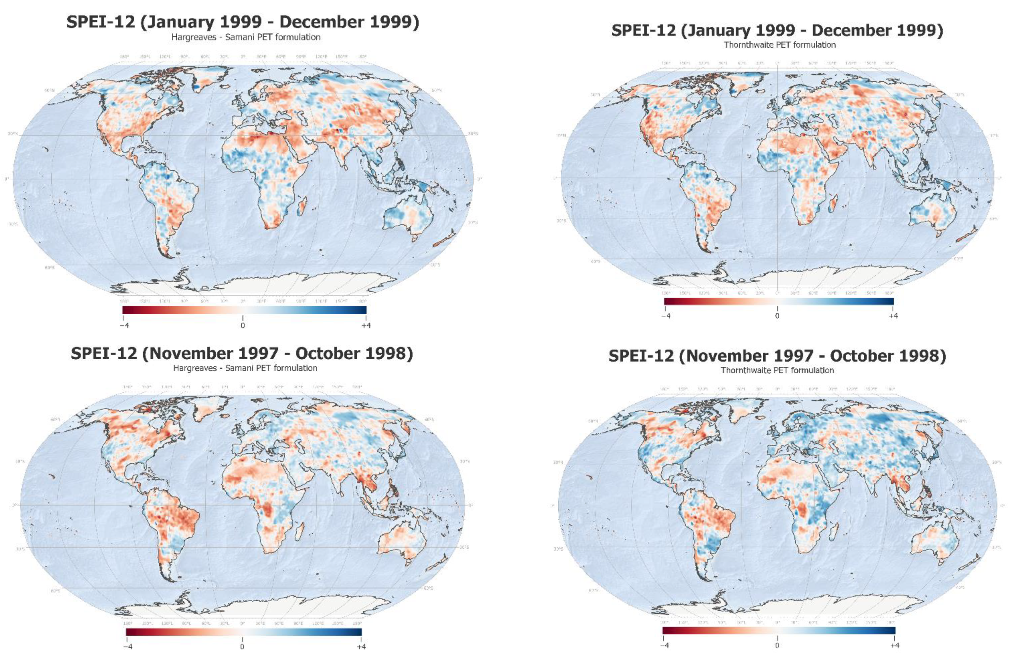
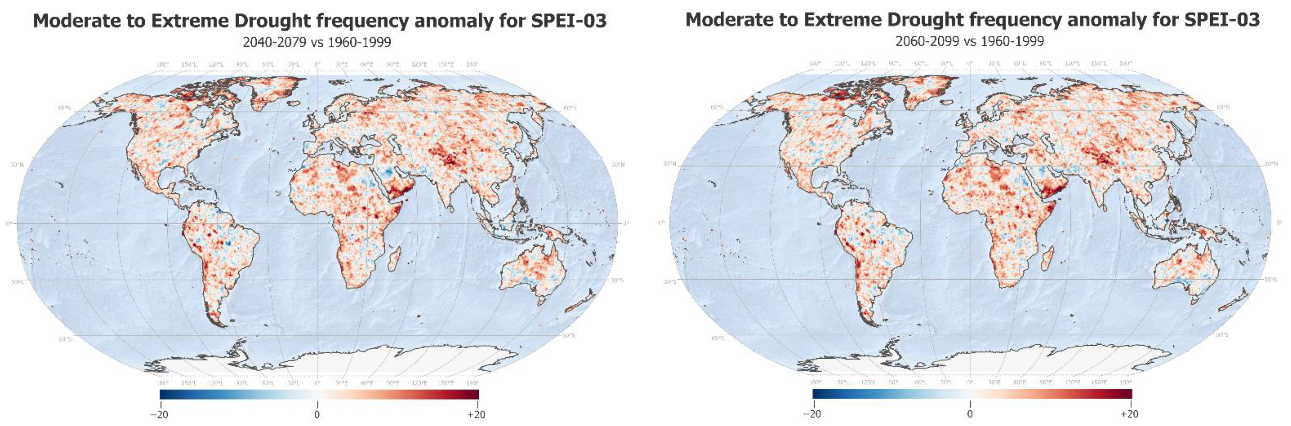
2.3. Data Description
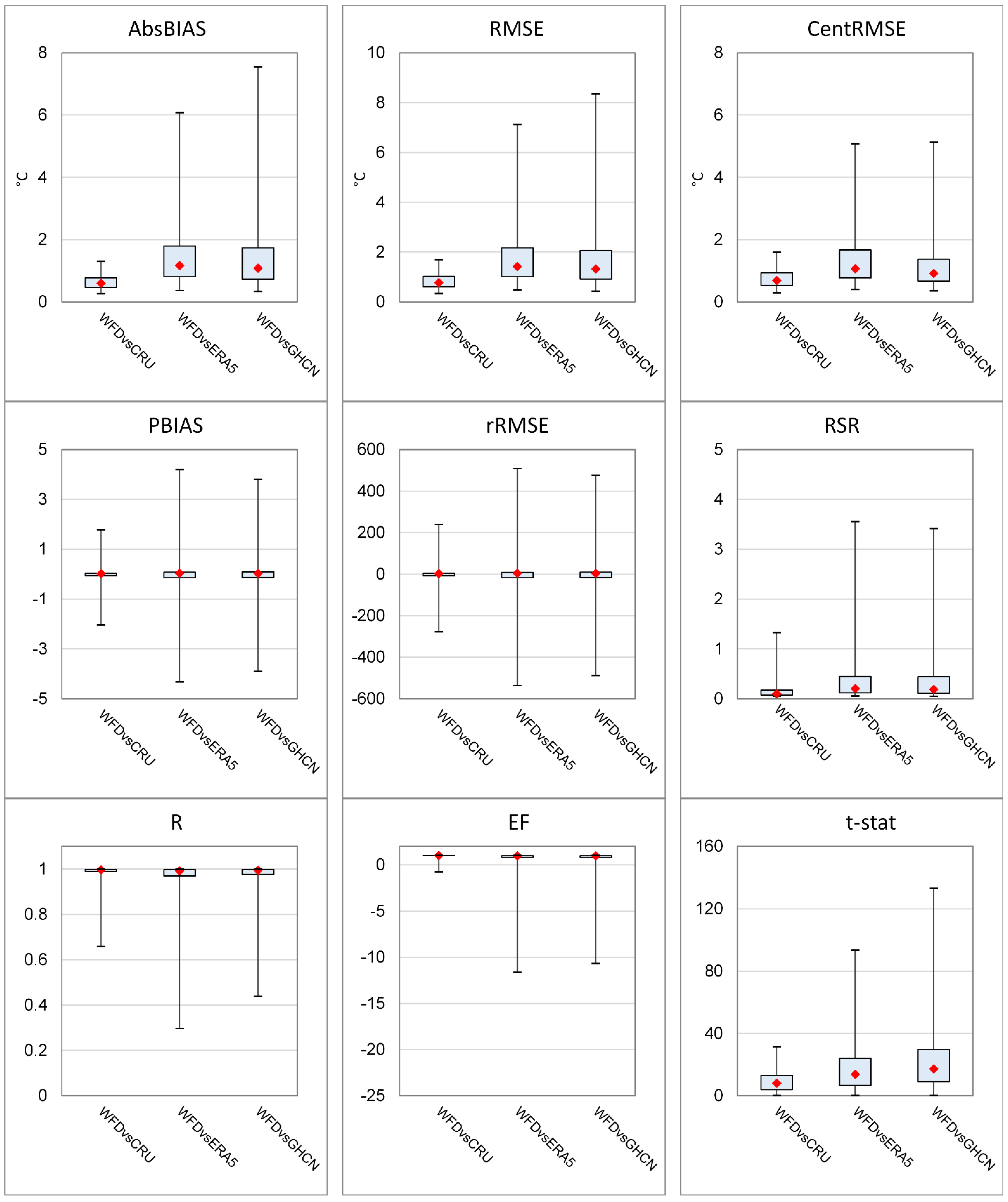
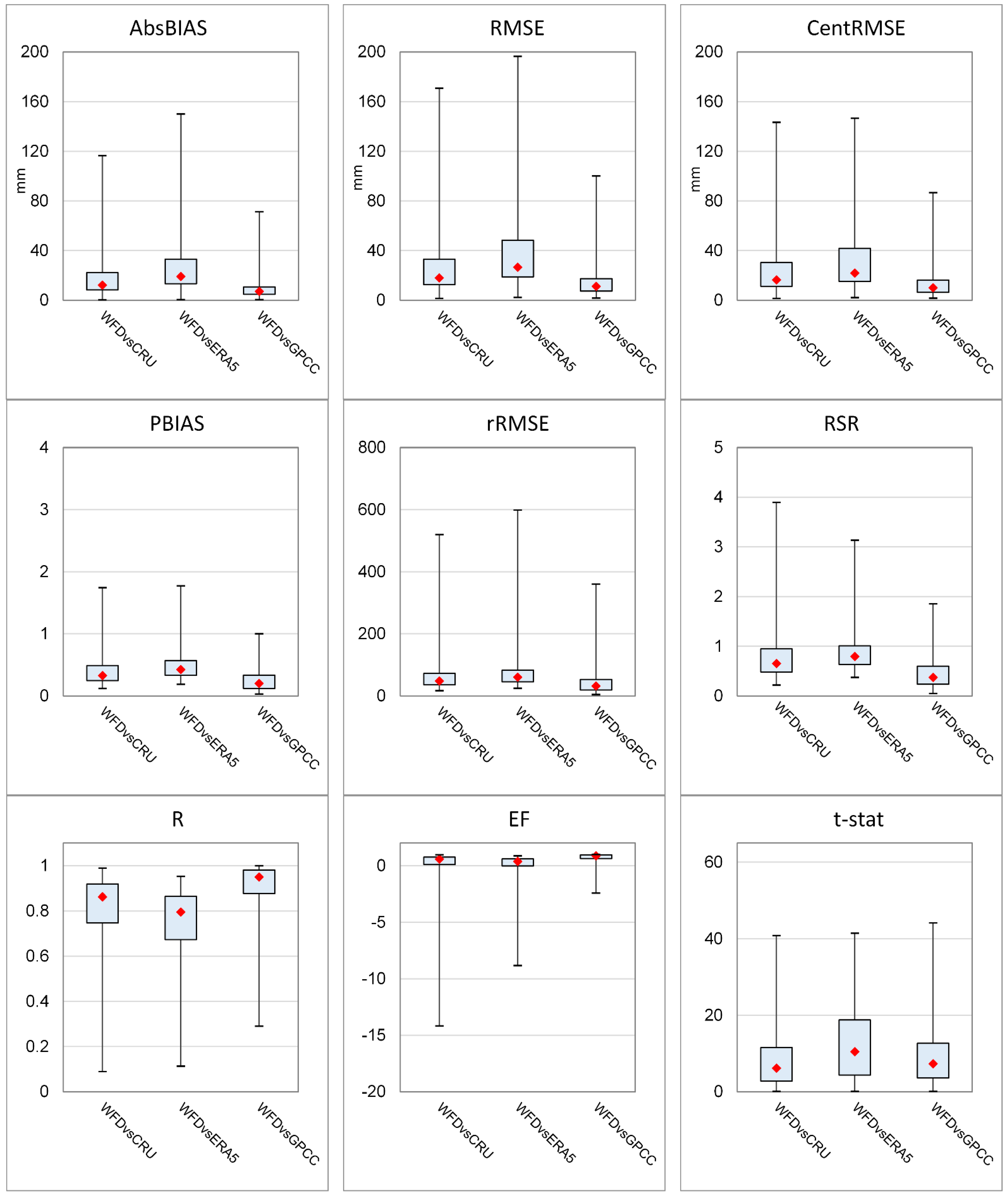
For each source dataset (WFD for the historical period and GCMs/ESMs for two future periods), each RCP (except RCP4.5 for CMCC-CESM), each period (1960–1999, 2040–2079, and 2060–2099), and each PET formulation, 18 maps were generated, representing the durations (i.e., from 1 to 18 consecutive months) considered in calculating the SPEI, i.e., the deviation from the average moisture conditions for the same timing and duration within the respective climatological period. In total, 828 files were generated, providing maps in the multidimensional NetCDF file format. Each file represents a regular spatial grid of 720 columns and 360 rows at 0.5° × 0.5° horizontal resolution and with 480 monthly time steps (12 months for 40 years) for each period. The time steps represent the ending month of the calculated SPEI, (e.g., the 3-month SPEI (SPEI-03) covering months from January to March is flagged as “March”).

2.4. Validation

Considering the nature of the presented dataset, the technical validation has to be interpreted as a comparison based on the variables underlying the SPEI calculation (i.e., temperature (T) and precipitation (P)) between the WFD and the most recent releases of well-consolidated climate datasets that are supposed to be improved at least in terms of the number of embedded observational data at the basis of the given spatialization approach.
Monthly time series of T and P from January 1960 to December 1999 from WFD were evaluated against paired time series of four datasets—GPCCv2018, GHCN-CAMS, CRU4.05, and ERA5—as described in Table 5, together with some comments about the level of independence to be considered in the evaluation. In the case of ERA5, the two datasets available at the time of writing, i.e., 1950–1978 and 1979–present, were merged.
The comparison among datasets for inputs P and T was preferred to directly for the SPEI in order to avoid obtaining good results for the wrong reasons (i.e., simultaneous under- or overestimation of P and T, leading to erroneously comparable P-PET time series between datasets) and to avoid depending on different (and thus not physically consistent) sources to ensure a comparison based on fully independent datasets for both P and T (see Table 5).
Nine performance indices were calculated according to the work of Santini and Caporaso [48]. In particular, like the work of Gudmundsson et al. [49], the correlation coefficient (R), the mean absolute bias (|Bias|), and the root mean square error (RMSE) were computed, with the |Bias| preferred to signed bias in order to avoid compensation of errors across months. The RMSE was also centered (CentRMSE) to make it independent of |Bias| [50]. The employed relative performance indices are the relative root square mean error (rRSME, %), as also applied by Nohara et al. [51]; the percentage absolute bias (P|Bias|) [50]; the ratio of RMSE to the standard deviation of observations (RSR [50]); and the model efficiency index (EF), also known as the Nash–Sutcliffe index [52]. Finally, the t-stat index, as adopted by Despotovic et al. [53], combines the squares of RMSE and of signed bias. All the indices are described in Table S1 in the Supplementary Materials.
Table 1. Characteristics of the main SPEI-based datasets, including those with future projections, those specific to particular regions, and those only based on observations or re-analysis. Concerning PET formulations: H = Hargreaves–Samani; T = Thornthwaite; PM = Penman–Monteith.
Ref.Spatial CoverageTemporal CoverageGCMs/ESMsScenariosDuration
(Months)
PET Formulation(s)
This
dataset
Global (0.5°)1960–1999; 2040–2079; 2060–209962 RCPs1 to 182 (H, T)
[14]Global (0.5°)1976–2005; 2030–208993 RCPs121 (PM)
[17]Global (0.5°)1986–2005; 2016–2035, 2046–206553 RCPs121 (PM)
[54]Global (1°)1961–2005; 2010–2054; 2055–2099151 RCP3, 6, 121 (T)
[55]Global (0.5°)1975–21001 RCM forced by some GCMs/ESMs1 RCP12N.A.
[56]Global
(0.44°)
1981–2100;
4 warming levels between 1 °C to 4 °C
16 to 145 GCMs/ESMs-RCMs chains based on the region2 RCPs121 (H)
[57]Global (0.5°)1961–2100;
8 warming levels between < +1 °C and +4 °C
23Pattern scaling approach121 (PM)
https://climate-scenarios.canada.ca/?page=spei; accessed on 3 February 2023Canada (1°)1900–2100303 RCPs1, 3, 121 (modified H [58])
[15]East Africa (0.5°)2011–2040; 2041–2070; 2071–210053 RCPs1, 3, 6, 121 (PM)
[59]China (0.0083°)1901–2100273 RCPs121 (H)
[60]Australia
(100 km)
1981–210094 RCPs 1 (H)
https://spei.csic.es/database.html; accessed on 3 February 2023Global (0.5°)1901–2020N.A.
(gridded observations)
1 to 481 (PM)
[61]Global (0.5°)1979–presentN.A.
(gridded reanalysis)
0.5, 1, 3, 6, 9, 12, 24, 36, 481 (PM)
[16]Africa
(5–50 km, function of the input dataset)
1981–2016N.A.
(gridded observations)
1 to 48Function of the input dataset method
[62]China (0.1°)1979–2018N.A.
(gridded observations)
1, 3, 12
(daily scale)
1 (H)
[18]China1961–2018N.A.
Station-based
1, 3, 6, 12, 241 (H)
[19]Central Asia (5–25 km, function of the input dataset)1981–2018N.A.
(gridded observations)
1 to 48Function of the input dataset method
Table 2. Global average of SPEI-03 values across all timings under different scenarios. ENS = ensemble among ESMs/GCMs; see Data Availability Statement for scenario naming.
ScenarioAverage SPEI-03
WFD_1960_1999_H0.006504
ENS_2040_2079_45_H0.004764
ENS_2040_2079_85_H0.004690
ENS_2060_2099_45_H0.004682
ENS_2060_2099_85_H0.004686
WFD_1960_1999_T0.005663
ENS_2040_2079_45_T0.004298
ENS_2040_2079_85_T0.003633
ENS_2060_2099_45_T0.004328
ENS_2060_2099_85_T0.003721
Table 3. Description of ESMs/GCMs used in this study.
Model (Code)Atmospheric Resolution (°lat × °lon)RCP
GFDL-ESM2M (GFDL)2° × 2.5°4.5, 8.5
HadGEM2-ES (MOHC)1.25° × 1.875°4.5, 8.5
IPSL-CM5A-LR (IPSL)1.875° × 3.75°4.5, 8.5
MIROC-ESM-CHEM (MIRO)2.8° × 2.8°4.5, 8.5
NorESM1-M (NESM)1.89° × 2.5°4.5, 8.5
CMCC-CESM (CMCC)3.44° × 3.75°8.5
Table 4. SPEI classification of severity classes.
Value ClassificationClass Description
SPEI ≤ −2Extremely dry
−2.0 < SPEI ≤ −1.5Severely dry
−1.5 < SPEI ≤ −1.0Moderately dry
−1.0 < SPEI ≤ 1.0Normally dry to wet
1.0 < SPEI ≤ 1.5Moderately wet
1.5 < SPEI ≤ 2.0Severely wet
SPEI > 2.0Extremely wet
Table 5. Description of the datasets used for validation of P and T.
DatasetWebsiteComments for Validation
GPCCv2018https://psl.noaa.gov/data/gridded/data.gpcc.html (accessed on 3 February 2023) [63]Used to validate P;
older GPCCv4 as the basis of WFD for P
GHCN_CAMShttps://psl.noaa.gov/data/gridded/data.ghcncams.html (accessed on 3 February 2023) [64]Used to validate T; fully independent dataset for T
CRU4.05https://crudata.uea.ac.uk/cru/data/hrg/cru_ts_4.05/ (accessed on 3 February 2023) [65]Used to validate P and T;
older CRU2.1 as the basis of WFD for T but a fully independent dataset for P
ERA5https://cds.climate.copernicus.eu/cdsapp#!/dataset/reanalysis-era5-land?tab=overview (accessed on 3 February 2023);
https://cds.climate.copernicus.eu/cdsapp#!/dataset/reanalysis-era5-single-levels-preliminary-back-extension?tab=overview (accessed on 3 February 2023) [66]
Used to validate P and T;
older ERA-40 as the basis of WFD for T and P
The box plots presented in Figure 3 show the statistical distribution of the nine performance indices at the global level based on the evaluation of the WFD temperature (T) against each of the three datasets reporting the same variable. Figure 4 is the same for precipitation (P).
Results for temperature (precipitation) show that, as expected, due to the dependence reported in Table 5, WFD is closer to the CRU (GPCC) dataset based on the different indices; however, the comparison against the ERA5 and the fully independent GHCN-CAMS (CRU) is also acceptable, with the ERA5 presenting the greatest differences from WFD in some cases, probably due to the large improvements made out since the ERA-40 and the assimilation of many other data in the latest generation reanalysis.
As an example of where deviations are concentrated, maps of the RMSE presenting high and wide interquartile ranges relative to the fully independent datasets (GHCN for T and CRU4 for P) are reported in the Supplementary Materials (Figure S1), revealing slightly lower performances in the intratropical latitudes for P and across limited spots, in particular over regions with the highest elevations for T.

3. User Notes

When using this SPEI dataset or part of it, please cite this manuscript. For any questions, suggestions, or requests for collaboration regarding this SPEI dataset, please contact the corresponding author. For example, besides data sources for the dataset presented in this manuscript, data from further climate simulations can be integrated, e.g., also considering RCPs 2.6 and 6.0 and/or additional models available from other ISIMIP rounds or bias-correction efforts. Additionally, performance index maps related to technical validation (see Section 2.4) are available from the authors upon request.
Data are in NetCDF4 format and can be viewed through Panoply developed in Java (http://www.giss.nasa.gov/tools/panoply/; accessed on 3 February 2023) or using other viewers such as ncBrowse, ncview, and nCDF_Browser. The easiest and fastest way to operate the NetCDF format is via command-/script-based languages such as CDO (Climate Data Operators) and NCO (NetCDF Operators) or through Python, MATLAB, or R. Some commercial GIS packages allow for reading and elaboration of NetCDF data, such as ArcGIS (from version 9.2 on) and IDRISI Taiga.
Other common interoperable formats (i.e., ESRI grid and GeoTIFF) can be requested by contacting the authors for a subselection of the dataset, the size of which will be defined based on the specific request from interested users and on the processing time needed.
Please consider that for SPEI durations of more than one month, the two starting years of each period can have one or more time steps, with no data for the whole spatial domain. This is due to the impossibility of calculating the SPEI; at the beginning of each long-term period, a function of the months is included because the SPEI is dated with the ending month of the consecutive months considered. Indeed, the first valid time step for the SPEI-XX duration is the month (XX) of the time series. For example, in case of SPEI-06, the first valid value is in June of the period’s start year; in the case of SPEI-18, the first valid value is in June of the period’s start year +1.
When using data related to future periods, please consider that in climatological studies, it is recommended to do not work with single dates (years or months) but rather to focus on statistics of the considered variable or derived indicator over the long term (at least 30 years, as recommended by the WMO guidelines (https://library.wmo.int/doc_num.php?explnum_id=4166; accessed on 3 February 2023).

Supplementary Materials

The following supporting information can be downloaded at: https://www.mdpi.com/article/10.3390/data8020036/s1, SupplementaryInformation.doc: PET formulations, performance indices, spatial distribution of RMSE with respect to independent datasets, and an example of CDO commands to use data. Table S1: Performance indices and related formulations [67,68]. Figure S1: Example maps of RMSE spatial distribution.

Author Contributions

Conceptualization, M.S.; methodology, M.S.; software, M.S. and L.C.; validation, M.S. and L.C.; formal analysis, M.S., L.C. and M.M.; data curation, M.S. and M.M.; writing—original draft preparation, M.S. and S.N.; writing—review and editing, M.S., S.N., M.M. and L.C.; visualization, M.S. and S.N.; supervision, M.S. All authors have read and agreed to the published version of the manuscript.

Funding

This research received no external funding.

Institutional Review Board Statement

Not Applicable.

Informed Consent Statement

Not applicable.

Data Availability Statement

The files representing the SPEI dataset were ingested in the CMCC Data Delivery System (DDS; https://dds.cmcc.it/; accessed on 3 February 2023) and are available under the Creative Commons License CC-BY. From the above URL, after login, the user can retrieve the SPEI dataset (https://doi.org/10.25424/cmcc-mfd5-t060; accessed on 3 February 2023) through the DDS Web Portal by selecting the product related to the historical period (historical) or the two future periods (future_2040_2079 and future_2060_2099). For each product, different parameters can be selected; pet indicates the PET formulation (H = Hargreaves–Samani, and T = Thornthwaite), model indicates the source climate dataset (CMCC, GFDL, IPSL, MIRO, MOHC, or NESM; see Table 2), scenario indicates the forcing RCP (RCP 4.5 (45) or RCP 8.5 (85)), and duration indicates the SPEI duration in months (ranging from 01 to 18). Finally, the user can select the months and years within the selected period and the spatial coverage—global or for a subregion—and can submit a request via the Web Portal or by using the DDS Python client (https://pypi.org/project/ddsapi; accessed on 3 February 2023); the result corresponding to the request can be downloaded as a NetCDF file. The “Request Download” option is activated only if the combination of selections is valid, i.e., it appears as deactivated for the default selection of CMCC under RCP 4.5 when accessing the dataset for future periods. The SPEI was calculated using the SPEIbase package (https://github.com/sbegueria/SPEIbase; accessed on 3 February 2023); outputs can be processed through CDO and NCO scripts. For example, the CDO commands used to derive Figure 2 (calculating the differences between the ensemble median of each of the two future periods vs. the historical period) are reported in the Supplementary Materials.

Acknowledgments

The authors are thankful for GPCC precipitation data provided by the NOAA/OAR/ESRL PSL, Boulder, Colorado, USA, which are available from their website at https://psl.noaa.gov/data/gridded/data.gpcc.html (accessed on 29 March 2022) and GHCN gridded V2 data provided by the NOAA/OAR/ESRL PSL, Boulder, CO, USA, which are available from their Web site at https://psl.noaa.gov/data/gridded/data.ghcncams.html (accessed on 29 March 2022). ERA5 reanalysis was accessed through the Copernicus Climate Change Service (C3S) Climate Data Store (CDS) (https://cds.climate.copernicus.eu/#!/home; accessed on 29 March 2022).

Conflicts of Interest

The authors declare no conflict of interest.

References

  1. Seneviratne, S.I.; Zhang, X. Weather and Climate Extreme Events in a Changing Climate. In Climate Change 2021: The Physical Science Basis. Contribution of Working Group I to the Sixth Assessment Report of the Intergovernmental Panel on Climate Change; Masson-Delmotte, V., Zhai, P., Pirani, A., Connors, S.L., Péan, C., Chen, Y., Goldfarb, L., Gomis, L.I., Matthews, J.B.R., Berger, S., Eds.; Cambridge University Press: Cambridge, UK; New York, NY, USA, 2021; pp. 1513–1766. [Google Scholar] [CrossRef]
  2. Wilhite, D.A.; Glantz, M.H. Understanding: The drought phenomenon: The role of definitions. Water Int. 1985, 10, 111–120. [Google Scholar] [CrossRef]
  3. Mishra, A.K.; Singh, V.P. A review of drought concepts. J. Hydrol. 2010, 391, 202–216. [Google Scholar] [CrossRef]
  4. Lloyd-Hughes, B. The impracticality of a universal drought definition. Theor. Appl. Clim. 2014, 117, 607–611. [Google Scholar] [CrossRef]
  5. Van Loon, A.F. Hydrological drought explained. Wiley Interdiscip. Rev. Water 2015, 2, 359–392. [Google Scholar] [CrossRef]
  6. Slette, I.J.; Post, A.K.; Awad, M.; Even, T.; Punzalan, A.; Williams, S.; Smith, M.D.; Knapp, A.K. How ecologists define drought, and why we should do better. Glob. Chang. Biol. 2019, 25, 3193–3200. [Google Scholar] [CrossRef] [PubMed]
  7. Crausbay, S.D.; Betancourt, J.; Bradford, J.; Cartwright, J.; Dennison, W.C.; Dunham, J.; Enquist, C.A.; Frazier, A.G.; Hall, K.R.; Littell, J.S.; et al. Unfamiliar Territory: Emerging Themes for Ecological Drought Research and Management. One Earth 2020, 3, 337–353. [Google Scholar] [CrossRef]
  8. Palmer, W.C. Meteorological Drought Research Paper No. 45; US Department of Commerce Weather Bureau: Washington, DC, USA, 1965; p. 58.
  9. Vicente-Serrano, S.M.; Beguería, S.; López-Moreno, J.I. A multiscalar drought index sensitive to global warming: The standardized precipitation evapotranspiration index. J. Clim. 2010, 23, 1696–1718. [Google Scholar] [CrossRef]
  10. Cook, B.I.; Smerdon, J.E.; Seager, R.; Coats, S. Global warming and 21st century drying. Clim. Dyn. 2014, 43, 2607–2627. [Google Scholar] [CrossRef]
  11. McKee, T.B.; Doesken, N.J.; Kleist, J. The Relationship of Drought Frequency and Duration to Time Scales. In Proceedings of the 8th Conference on Applied Climatology, Anaheim, CA, USA, 17–22 January 1993; American Meteorological Society: Boston, MA, USA, 1993. [Google Scholar]
  12. Vicente-Serrano, S.M.; Beguería, S.; López-Moreno, J.I. Global changes in drought conditions under different levels of warming. Geophys. Res. Lett. 2018, 45, 3285–3296. [Google Scholar] [CrossRef]
  13. Zhao, T.; Dai, A. Uncertainties in historical changes and future projections of drought. Part II: Model-simulated historical and future drought changes. Clim. Chang. 2016, 144, 535–548. [Google Scholar] [CrossRef]
  14. Lu, Y.; Cai, H.; Jiang, T.; Sun, S.; Wang, Y.; Zhao, J.; Yu, X.; Sun, J. Assessment of global drought propensity and its impacts on agricultural water use in future climate scenarios. Agric. For. Meteorol. 2019, 278, 107623. [Google Scholar] [CrossRef]
  15. Haile, G.G.; Tang, Q.; Hosseini-Moghari, S.; Liu, X.; Gebremicael, T.G.; Leng, G.; Kebede, A.; Xu, X.; Yun, X. Projected impacts of climate change on drought patterns over East Africa. Earth’s Future 2020, 8, e2020EF001502. [Google Scholar] [CrossRef]
  16. Peng, J.; Dadson, S.; Hirpa, F.; Dyer, E.; Lees, T.; Miralles, D.G.; Vicente-Serrano, S.M.; Funk, C. A pan-African high-resolution drought index dataset. Earth Syst. Sci. Data 2020, 12, 753–769. [Google Scholar] [CrossRef]
  17. Liu, Y.; Chen, J. Future global socioeconomic risk to droughts based on estimates of hazard, exposure, and vulnerability in a changing climate. Sci. Total Environ. 2021, 751, 142159. [Google Scholar] [CrossRef] [PubMed]
  18. Wang, Q.; Zeng, J.; Qi, J.; Zhang, X.; Zeng, Y.; Shui, W.; Xu, Z.; Zhang, R.; Wu, X.; Cong, J. A multi-scale daily SPEI dataset for drought characterization at observation stations over mainland China from 1961 to 2018. Earth Syst. Sci. Data 2021, 13, 331–341. [Google Scholar] [CrossRef]
  19. Pyarali, K.; Peng, J.; Disse, M.; Tuo, Y. Development and application of high resolution SPEI drought dataset for Central Asia. Sci. Data 2022, 9, 172. [Google Scholar] [CrossRef]
  20. Warszawski, L.; Frieler, K.; Huber, V.; Piontek, F.; Serdeczny, O.; Schewe, J. The Inter-Sectoral Impact Model Intercomparison Project (ISI-MIP): Project framework. Proc. Natl. Acad. Sci. USA 2014, 111, 3228–3232. [Google Scholar] [CrossRef]
  21. Collins, M. Ensembles and probabilities: A new era in the prediction of climate change. Philos. Trans. R. Soc. 2007, 365, 1957–1970. [Google Scholar] [CrossRef]
  22. Subedi, A.; Chávez, J.L. Crop Evapotranspiration (ET) Estimation Models: A Review and Discussion of the Applicability and Limitations of ET Methods. J. Agric. Sci. 2015, 7, 50–68. [Google Scholar] [CrossRef] [Green Version]
  23. Vicente-Serrano, S.M.; Azorin-Molina, C.; Sanchez-Lorenzo, A.; Revuelto, J.; Lopez-Moreno, J.I.; Gonzalez-Hidalgo, J.C.; Morán-Tejeda, E.; Espejo, F. Reference evapotranspiration variability and trends in Spain, 1961–2011. Glob. Planet. Chang. 2014, 121, 26–40. [Google Scholar] [CrossRef]
  24. Weedon, G.P.; Gomes, S.; Viterbo, P.; Shuttleworth, W.J.; Blyth, E.; Österle, H.; Adam, J.C.; Bellouin, N.; Boucher, O.; Best, M. Creation of the WATCH Forcing Data and Its Use to Assess Global and Regional Reference Crop 309 Evaporation over Land during the Twentieth Century. J. Hydrometeorol. 2011, 12, 823–848. [Google Scholar] [CrossRef]
  25. Hadley Centre for Climate Prediction and Research/Met Office/Ministry of Defence/United Kingdom. WATer and Global Change (WATCH) Forcing Data (WFD)—20th Century. Research Data Archive at the National Center for Atmospheric Research, Computational and Information Systems Laboratory (2018). Available online: https://doi.org/10.5065/1B5Z-KQ51 (accessed on 28 January 2023).
  26. Uppala, S.M.; Kållberg, P.W.; Simmons, A.J.; Andrae, U.; Da Costa Bechtold, V.; Fiorino, M.; Gibson, J.K.; Haseler, J.; Hernandez, A.; Kelly, G.A.; et al. The ERA-40 re-analysis. Q. J. R. Meteorol. Soc. 2005, 131, 2961–3012. [Google Scholar] [CrossRef]
  27. Piani, C.; Weedon, G.; Best, M.; Gomes, S.; Viterbo, P.; Hagemann, S.; Haerter, J. Statistical bias correction of global simulated daily precipitation and temperature for the application of hydrological models. J. Hydrol. 2010, 395, 199–215. [Google Scholar] [CrossRef]
  28. Taylor, K.E.; Stouffer, R.J.; Meehl, G.A. An overview of CMIP5 and the experiment design. Bull. Am. Meteorol. Soc. 2012, 93, 485–498. [Google Scholar] [CrossRef]
  29. van Vuuren, D.P.; Edmonds, J.; Kainuma, M.; Riahi, K.; Thomson, A.; Hibbard, K.; Hurtt, G.C.; Kram, T.; Krey, V.; Lamarque, J.-F.; et al. The representative concentration pathways: An overview. Clim. Chang. 2011, 109, 5–31. [Google Scholar] [CrossRef]
  30. Ehret, U.; Zehe, E.; Warrach-Sagi, K.; Liebert, J. HESS Opinions “Should we apply bias correction to global and regional climate model data? ”. Hydrol. Earth Syst. Sci. 2012, 16, 3391–3404. [Google Scholar] [CrossRef]
  31. Hempel, S.; Frieler, K.; Warszawski, L.; Schewe, J.; Piontek, F. A trend-preserving bias correction—The ISI-MIP approach. Earth Syst. Dynam. 2013, 4, 219–236. [Google Scholar] [CrossRef]
  32. Cherchi, A.; Fogli, P.G.; Lovato, T.; Peano, D.; Iovino, D.; Gualdi, S.; Masina, S.; Scoccimarro, E.; Materia, S.; Bellucci, A.; et al. Global Mean Climate and Main Patterns of Variability in the CMCC-CM2 Coupled Model. J. Adv. Model. Earth Syst. 2019, 11, 185–209. [Google Scholar] [CrossRef]
  33. Vichi, M.; Manzini, E.; Fogli, P.G.; Alessandri, A.; Patara, L.; Scoccimarro, E.; Masina, S.; Navarra, A. Global and regional ocean carbon uptake and climate change: Sensitivity to a substantial mitigation scenario. Clim. Dyn. 2011, 37, 1929–1947. [Google Scholar] [CrossRef]
  34. Thomson, A.M.; Calvin, K.V.; Smith, S.J.; Kyle, G.P.; Volke, A.; Patel, P.; Delgado-Arias, S.; Bond-Lamberty, B.; Wise, M.A.; Clarke, L.E.; et al. RCP4.5: A pathway for stabilization of radiative forcing by 2100. Clim. Chang. 2011, 109, 77–94. [Google Scholar] [CrossRef]
  35. Riahi, K.; Rao, S.; Krey, V.; Cho, C.; Chirkov, V.; Fischer, G.; Kindermann, G.E.; Nakicenovic, N.; Rafaj, P. RCP 8.5-A scenario of comparatively high greenhouse gas emissions. Clim. Chang. 2011, 109, 33–57. [Google Scholar] [CrossRef]
  36. Hargreaves, G.H. Estimating Potential Evapotranspiration. J. Irrig. Drain. Div. 1982, 108, 225–230. [Google Scholar] [CrossRef]
  37. Thornthwaite, C.W. An approach toward a rational classification of climate. Geogr. Rev. 1948, 38, 55–94. [Google Scholar] [CrossRef]
  38. Almorox, J.; Quej, V.H.; Martí, P. Global performance ranking of temperature-based approaches for evapotranspiration estimation considering Köppen climate classes. J. Hydrol. 2015, 528, 514–522. [Google Scholar] [CrossRef]
  39. Bai, P.; Liu, X.; Yang, T.; Li, F.; Liang, K.; Hu, S.; Liu, C. Assessment of the Influences of Different Potential Evapotranspiration Inputs on the Performance of Monthly Hydrological Models under Different Climatic Conditions. J. Hydrometeorol. 2016, 17, 2259–2274. [Google Scholar] [CrossRef]
  40. Ceglar, A.; Zampieri, M.; Gonzalez-Reviriego, N.; Ciais, P.; Schauberger, B.; Van Der Velde, M. Time-varying impact of climate on maize and wheat yields in France since 1900. Environ. Res. Lett. 2020, 15, 094039. [Google Scholar] [CrossRef]
  41. Kukal, M.S.; Irmak, S. Climate-Driven Crop Yield and Yield Variability and Climate Change Impacts on the U.S. Great Plains Agricultural Production . Sci. Rep. 2018, 8, 3450. [Google Scholar] [CrossRef] [PubMed]
  42. Liu, D.; Mishra, A.K.; Ray, D.K. Sensitivity of global major crop yields to climate variables: A non-parametric elasticity analysis. Sci. Total Environ. 2020, 748, 141431. [Google Scholar] [CrossRef] [PubMed]
  43. Matiu, M.; Ankerst, D.P.; Menzel, A. Interactions between temperature and drought in global and regional crop yield variability during 1961-2014. PLoS ONE 2017, 12, e0178339. [Google Scholar] [CrossRef] [Green Version]
  44. Ray, D.K.; Gerber, J.S.; MacDonald, G.K.; West, P.C. Climate variation explains a third of global crop yield variability. Nat. Commun. 2015, 6, 5989. [Google Scholar] [CrossRef]
  45. Vogel, E.; Donat, M.G.; Alexander, L.V.; Meinshausen, M.; Ray, D.K.; Karoly, D.; Meinshausen, N.; Frieler, K. The effects of climate extremes on global agricultural yields. Environ. Res. Lett. 2019, 14, 054010299. [Google Scholar] [CrossRef]
  46. Zampieri, M.; Ceglar, A.; Dentener, F.; Toreti, A. Wheat yield loss attributable to heat waves, drought and water excess at the global, national and subnational scales. Environ. Res. Lett. 2017, 12, 064008. [Google Scholar] [CrossRef]
  47. Santini, M.; Noce, S.; Antonelli, M.; Caporaso, L. Complex drought patterns robustly explain global yield loss for major crops. Sci. Rep. 2022, 12, 5792. [Google Scholar] [CrossRef] [PubMed]
  48. Santini, M.; Caporaso, L. Evaluation of Freshwater Flow From Rivers to the Sea in CMIP5 Simulations: Insights From the Congo River Basin. J. Geophys. Res. Atmos. 2018, 123, 10278–10300. [Google Scholar] [CrossRef]
  49. Gudmundsson, L.; Tallaksen, L.M.; Stahl, K.; Clark, D.; Dumont, E.; Hagemann, S.; Bertrand, N.; Gerten, D.; Heinke, J.; Hanasaki, N.; et al. Comparing large-scale hydrological model simulations to observed runoff percentiles in Europe. J. Hydrometeorol. 2011, 13, 604–620. [Google Scholar] [CrossRef]
  50. Yang, H.; Piao, S.; Zeng, Z.; Ciais, P.; Yin, Y.; Friedlingstein, P.; Sitch, S.; Ahlström, A.; Guimberteau, M.; Huntingford, C.; et al. Multicriteria evaluation of discharge simulation in dynamic global vegetation models. J. Geophys. Res. Atmos. 2015, 120, 7488–7505. [Google Scholar] [CrossRef]
  51. Nohara, D.; Kitoh, A.; Hosaka, M.; Oki, T. Impact of climate change on river discharge projected by multimodel ensemble. J. Hydrometeorol. 2006, 7, 1076–1089. [Google Scholar] [CrossRef]
  52. Nash, J.E.; Sutcliffe, J.V. River flow forecasting through conceptual models, part I—A discussion of principles. J. Hydrol. 1970, 10, 282–290. [Google Scholar] [CrossRef]
  53. Despotovic, M.; Nedic, V.; Despotovic, D.; Cvetanovic, S. Evaluation of empirical models for predicting monthly mean horizontal diffuse solar radiation. Renew. Sust. Energ. Rev. 2016, 56, 246–260. [Google Scholar] [CrossRef]
  54. Touma, D.; Ashfaq, M.; Nayak, M.A.; Kao, S.-C.; Diffenbaugh, N.S. A multi-model and multi-index evaluation of drought characteristics in the 21st century. J. Hydrol. 2015, 526, 196–207. [Google Scholar] [CrossRef]
  55. Naumann, G.; Alfieri, L.; Wyser, K. High Resolution SPEI Monthly Projection for the Globe (1975-2100). European Commission, Joint Research Centre (JRC), 2017. Available online: http://data.europa.eu/89h/jrc-climate-spei-drought-helix-ec-earth-1975-2100 (accessed on 3 February 2023).
  56. Spinoni, J.; Barbosa, P.; Bucchignani, E.; Cassano, J.; Cavazos, T.; Cescatti, A.; Christensen, J.H.; Christensen, O.B.; Coppola, E.; Evans, J.P.; et al. Global exposure of population and land-use to meteorological droughts under different warming levels and SSPs: A CORDEX-based study. Int. J. Climatol. 2021, 41, 6825–6853. [Google Scholar] [CrossRef]
  57. Price, J.; Warren, R.; Forstenhäusler, N.; Wallace, C.; Jenkins, R.; Osborn, T.J.; Van Vuuren, D.P. Quantification of meteorological drought risks between 1.5 °C and 4 °C of global warming in six countries. Clim. Chang. 2022, 174. [Google Scholar] [CrossRef]
  58. Droogers, P.; Allen, R.G. Estimating Reference Evapotranspiration Under Inaccurate Data Conditions. Irrig. Drain. Syst. 2002, 16, 33–45. [Google Scholar] [CrossRef]
  59. Ding, Y.; Peng, S. Spatiotemporal Trends and Attribution of Drought across China from 1901–2100. Sustainability 2020, 12, 477. [Google Scholar] [CrossRef]
  60. Araujo, D.S.A.; Marra, F.; Merow, C.; Nikolopoulos, E. Today’s 100 year droughts in Australia may become the norm bythe end of the century. Environ. Res. Lett. 2022, 17, 044034. [Google Scholar] [CrossRef]
  61. Vicente-Serrano, S.M.; Domínguez-Castro, F.; Reig, F.; Tomas-Burguera, M.; Peña-Angulo, D.; Latorre, B.; Beguería, S.; Rabanaque, I.; Noguera, I.; Lorenzo-Lacruz, J.; et al. A global drought monitoring system and dataset based on ERA5 reanalysis: A focus on crop- growing regions. Geosci. Data J. 2022, 1, 1–14. [Google Scholar] [CrossRef]
  62. Zhang, R.; Bento, V.A.; Qi, J.; Xu, F.; Wu, J.; Qiu, J.; Li, J.; Shui, W.; Wang, Q. The first high spatial resolution multi-scale daily SPI and SPEI raster dataset for drought monitoring and evaluating over China from 1979 to 2018. Big Earth Data 2023. [Google Scholar] [CrossRef]
  63. Schneider, U.; Becker, A.; Finger, P.; Meyer-Christoffer, A.; Rudolf, B.; Ziese, M. GPCC Full Data Reanalysis Version 6.0 at 0.5°: Monthly Land-Surface Precipitation from Rain-Gauges Built on GTS-Based and Historic Data; Global Precipitation Climatology Centre: Boulder, NV, USA, 2011. [Google Scholar] [CrossRef]
  64. Fan, Y.; van den Dool, H. A global monthly land surface air temperature analysis for 1948-present. J. Geophys. Res. Atmos. 2008, 113, D01103. [Google Scholar] [CrossRef]
  65. Harris, I.; Osborn, T.J.; Jones, P.; Lister, D. Version 4 of the CRU TS monthly high-resolution gridded multivariate climate dataset. Sci. Data 2020, 7, 109. [Google Scholar] [CrossRef]
  66. Hersbach, H.; Bell, B.; Berrisford, P.; Hirahara, S.; Horanyi, A.; Muñoz-Sabater, J.; Nicolas, J.; Peubey, C.; Radu, R.; Schepers, D.; et al. The ERA5 global reanalysis. Q. J. R. Meteorol. Soc. 2020, 146, 1999–2049. [Google Scholar] [CrossRef]
  67. Li, M.F.; Tang, X.P.; Wu, W.; Liu, H.B. General models for estimating daily global solar radiation for different solar radiation zones in mainland China. Energy Convers. Manag. 2013, 70, 139–148. [Google Scholar] [CrossRef]
  68. Moriasi, D.N. Model evaluation guidelines for systematic quantification of accuracy in watershed simulations. Trans. ASABE 2007, 50, 885–900. [Google Scholar] [CrossRef]
Figure 1. Example of the dataset for the 12-month SPEI (SPEI-12) from January 1999 to December 1999 (top panels, corresponding to a strong La Niña event) and from November 1997 to October 1998 (bottom panels, corresponding to a very strong El Niño event) under PET calculated by Hargreaves–Samani (left panels) and Thornthwaite (right panels) equations.
Data 08 00036 g001
Figure 2. Example of possible dataset elaboration to derive anomalies in the frequency (number of occurrences) of moderate-to-extreme droughts (SPEI ≤ −1; see Section 2.2) according to 3-month SPEI (SPEI-03) for the mid-term (2040–2079, (left)) and long-term (2060–2099, (right)) periods with respect to the historical period (1960–1999).
Data 08 00036 g002
Figure 3. Statistical distribution of the performance indices used in the comparison between WFD and the other datasets for temperature (CRU, ERA5, and GHCN) for the period of 1960–1999. Red symbols represent the median, box edges are the 25th and 75th percentiles, and the whiskers are the 0.7th and 99.3rd percentiles.
Data 08 00036 g003
Figure 4. Statistical distribution of the performance indices used in the comparison between WFD and the other datasets for precipitation (CRU, ERA5, and GPCC) during the period of 1960–1999. Red symbols represent the median, box edges are the 25th and 75th percentiles, and the whiskers are the 0.7th and 99.3rd percentiles.
Data 08 00036 g004
Disclaimer/Publisher’s Note: The statements, opinions and data contained in all publications are solely those of the individual author(s) and contributor(s) and not of MDPI and/or the editor(s). MDPI and/or the editor(s) disclaim responsibility for any injury to people or property resulting from any ideas, methods, instructions or products referred to in the content.

