Classification of Building Types in Germany: A Data-Driven Modeling Approach

Abstract

Details on building levels play an essential part in a number of real-world application models. Energy systems, telecommunications, disaster management, the internet-of-things, health care, and marketing are a few of the many applications that require building information. The essential variables that most of these models require are building type, house type, area of living space, and number of residents. In order to acquire some of this information, this paper introduces a methodology and generates corresponding data. The study was conducted for specific applications in energy system modeling. Nonetheless, these data can also be used in other applications. Building locations and some of their details are openly available in the form of map data from OpenStreetMap (OSM). However, data regarding building types (i.e., residential, industrial, office, single-family house, multi-family house, etc.) are only partially available in the OSM dataset. Therefore, a machine learning classification algorithm for predicting the building types on the basis of the OSM buildings’ data was introduced. Although the OSM dataset is the fundamental and most crucial one used for modeling, the machine learning algorithm’s training was performed on a dataset that was prepared by combining several features from three other datasets. The generated dataset consists of approximately 29 million buildings, of which about 19 million are residential, with 72% being single-family houses and the rest multi-family ones that include two-family houses and apartment buildings. Furthermore, the results were validated through a comparison with publicly available statistical data. The comparison of the resulting data with official statistics reveals that there is a percentage error of 3.64% for residential buildings, 13.14% for single-family houses, and −15.38% for multi-family houses classification. Nevertheless, by incorporating the building types, this dataset is able to complement existing building information in studies in which building type information is crucial.

1. Introduction

Real-world application models take account of the facts concerning buildings and their details [1,2]. The energy system model is one such application that uses building-level information. Energy systems are undergoing extensive transformations in an effort to reduce carbon dioxide (CO₂) emissions. Consequently, renewable energy sources (RES) are being widely introduced into energy mixes. Evaluating the optimal integration of RES necessitates better enumeration of total energy consumption. Building energy consumption accounts for a significant proportion of the total energy consumed. Therefore, estimating energy consumption in buildings necessitates building-level information (e.g., building type, number of residents, living space, etc.). Unfortunately, detailed information with respect to buildings is not publicly available.

However, despite containing detailed building information, synthetic data on buildings, apartments, families, households, and populations are openly available [3]. The synthetic data for Germany were produced from a survey conducted as part of the country’s 2011 census. Moreover, these data were aggregated for 100-m and one-kilometer grid cells. Each cell (100 m × 100 m) conveyed information about the buildings within it (i.e., the total number of each type, the identity of each cell, etc.). Nevertheless, data on the total number of buildings within the cells do not offer critical information regarding each of them. Therefore, building type classification of the building footprints is required.

Several studies have been conducted to date using a variety of classification approaches for building types. The classification of building types can be performed manually or automatically. As previously stated, surveying methods provide information about buildings (i.e., manually). However, this process requires a significant amount of time and human effort. Thus, automatic classification is the best method available at the moment. Advancements in remote sensing technology have enabled the extraction of physical features of buildings such as textures, geometries, size, and shape from remotely sensed images at low, medium, high, and very high resolution [4]. Additionally, light detection and ranging (LiDAR) offers the building’s height information, which is missing from the image data [5]. However, these building characteristics are retrieved through the use of machine learning or deep learning models. In addition to these features, the building footprints are gathered using edge-based geometric grouping or object-based classification [6]. The labeling of buildings or the classification of building types were accomplished in [5,7,8,9,10,11,12,13,14,15,16,17] using the datasets produced from the aforementioned approaches using remote sensed images, google earth images [18,19] and LiDAR data. Ref. [20] employs machine learning models to categorize buildings into single-family houses, multi-family houses, and non-residential buildings by utilizing LiDAR extracted data, including height and shape. Similarly, ref. [5,8,13] classified buildings as low-rise [5], multi-storey [13], high-rise [13], apartment [5], residential [8], non-buildings [5], and various commercial buildings [8]. Additionally, semantic labeling [6,12,21] and ontology-based categorization [7] were performed on the remote sensing data to identify building footprints as residential, non-residential, industrial, or factory. Here, several supervised machine learning techniques were used in these studies, including Random Forest [5,6,8], Support Vector Machines (SVM) [8], and deep learning methods [12]. Apart from supervised machine learning techniques, ref. [9,15] used unsupervised machine learning techniques to cluster settlement types based on the spatial pattern of building footprints. However, because the experts’ high degree of semantics highlights a semantic gap in the remote sensed imaging data [7], Point-of-Interest (POI) data (i.e., specific point location, e.g., hospital, office, restaurant, etc.), which is often user-generated data, was mapped to the remote sensed data to identify building types [10,11]. In this context, ref. [10] used remote sensing imagery and point-of-interest data to increase the accuracy and completeness of classification tasks. In addition to the POI data, ref. [14] identified residential and industrial buildings using nighttime light data and land cover data.

However, due to the complexity of image object extraction and classification in the remote sensing technique, several researchers are concentrating their research on classifying building types using geospatial vector data (i.e., points, lines, and polygons) [22]. To categorize different types of buildings, ref. [22,23,24,25,26,27,28,29] included geospatial vector data gathered and maintained by national mapping agencies [25], real estate cadasters [23], government agencies [22,24], commercial data suppliers, and web mapping services [4,30,31]. Additionally, ref. [32] recommended using taxi and population density statistics to identify building functions. However, due to the scarcity of data from remote sensing, point-of-interest data, commercial geospatial vector data, and human activity data, the researchers are classifying buildings using data from web mapping services. The web mapping services include not only the footprints of buildings, but also point-of-information data such as addresses, building usage, building type, and building functionality, as well as other information about the buildings. In this context, several prior research [4,30,33,34,35,36,37,38] identified building types using web mapping services such as OpenStreetMap (OSM) [39,40], Google maps, Gaode Maps, and Baidu Maps [4,35]. For instance, ref. [35] classified residential and numerous non-residential types using geographical data and POI data from Gaode and Baidu Maps. Additionally, ref. [33] used OSM’s building footprints and POI data to identify residential and non-residential buildings suitable for pesticide spraying to aid with malaria prevention. This clearly implies that building type information is beneficial not just for energy, transportation, and marketing objectives, but also for the health sector in light of the current global crisis.

In summary, extracting building type information from remote sensing methods needs a significant amount of computational power when executing global or even country-level classification and object segmentation tasks. Additionally, managing and retrieving image data for such a large spatial coverage is implausible. Furthermore, acquiring geographic vector data and POI data from commercial and government agencies is always subject to constraints and limitations. Additionally, human activity data is always a source of concern when it comes to privacy. As a result, volunteer-generated open map data from OSM is now the best option for utilizing and classifying building types. The OSM dataset provides building footprints (instead of data acquired from images by remote sensing) and POI data (alternative to POI data from commercial data providers and government agencies). However, according to [27], the incompleteness and discrepancies in OSM data are particularly noticeable. According to the results of the analysis of data collected from OSM, it has been discovered that the data is still incomplete, with several missing values; see Section 3.

To address the limitations mentioned above; this study developed a means of predicting the building type for each building extracted from the OSM data as accurately as possible. In order to perform this task effectively, several additional features have been added to the OSM data from various datasets. The most significant datasets bolstering the OSM data are Coordination of Information on the Environment (CORINE) [41], the height of buildings in Berlin [42], and 2011 census data for Germany [3]. The work conducted herein was motivated by a need for geo-referenced building location data and their labels, which could be used in several real-world applications. Moreover, the work conducted attempts to fill some of the gaps in the literature by classifying building types through the application of state-of-the-art machine learning algorithms to the incomplete dataset extracted from OSM. This study also addresses the challenges with respect to missing values and class imbalances in the datasets by pursuing the following objectives: (1) To extract building data with all of the corresponding features (e.g., geometry, area, address, tags, etc.); (2) to perform data analysis on the extracted data in order to quantify missing data; (3) to integrate additional features from the above-mentioned additional sources; and (4) to use sophisticated machine learning algorithms in order to classify building types with missing values and rectify class imbalances in the dataset.

The structure of the paper is as follows: the dataset is described in Section 2. Section 3 presents the data extraction, analysis, and preprocessing steps followed. This section also includes the application of a machine learning algorithm to the processed dataset. In addition, the results and validation of the tagged buildings are outlined. Section 4 provides the discussion concerning the method, application of the results, and the limitations. Finally, Section 5 conveys the conclusions and user notes regarding data usage.

2. Data Description

Prior to beginning the methods, this section describes the generated dataset with building types classified for Germany. The dataset was explicitly generated for Germany due to the requirement of building labels for developing geo-referenced synthetic electrical distribution grids in the country. However, the developed methodology can be applied to the generating of a dataset in any country. The dataset was provided in the GeoJSON file format. For the geographical features, the coordinate reference system used was the World Geodetic System 1984 (WGS 84) (EPSG:3857)—the original coordinate reference system of OSM data. The dataset comprises the attributes listed below.

The main features from the OSM data are as follows:

• osm_id (numerical): unique identity for each building footprint (e.g., 208594362, 107204221, 208593145, etc.).
• way_area (numerical): area of the building footprint in Mercator square meter obtained from original OSM data projection (e.g., 377, 2218.18, 493.99, 490.901, etc.).
• amenity_real (categorical): facility of buildings tagged in OSM (e.g., office, shop, leisure, construction site, supermarket, grocery, etc.).
• building_type (categorical): building tag originally tagged in OSM (e.g., yes, commercial, garage, terrace, office, train station, etc.).
• area (numerical): area of the building footprint when projected on ETRS89 (i.e., EPSG:3035).
• geometry (geometry): geometry for each building (EPSG:3857).

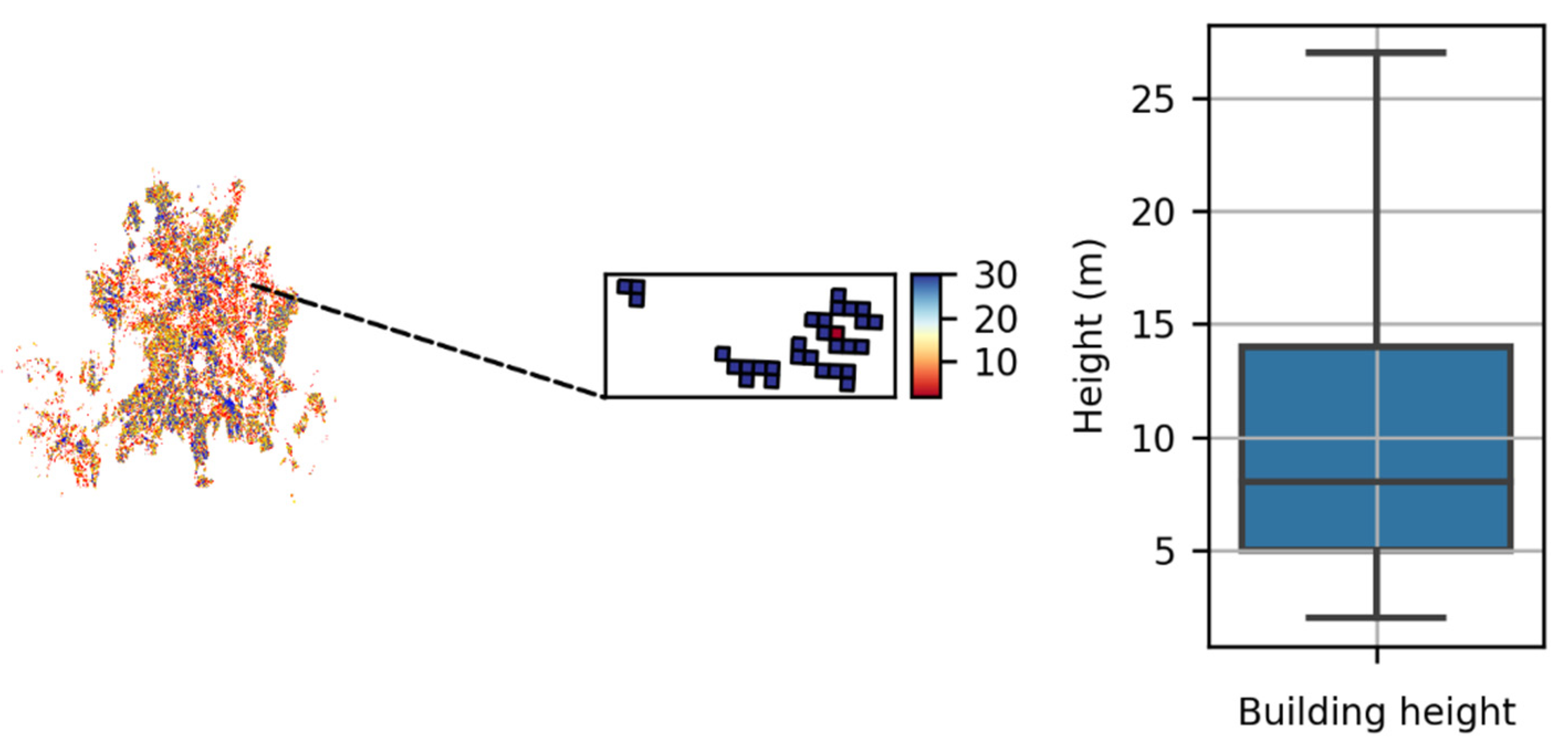
In addition, the height of each building was considered with respect to the heights dataset for Berlin public buildings.

• height (numerical): height of each building in Berlin (e.g., 4, 5, 10, etc.).

Furthermore, in order to improve the model’s performance, additional features from the Corine dataset were considered:

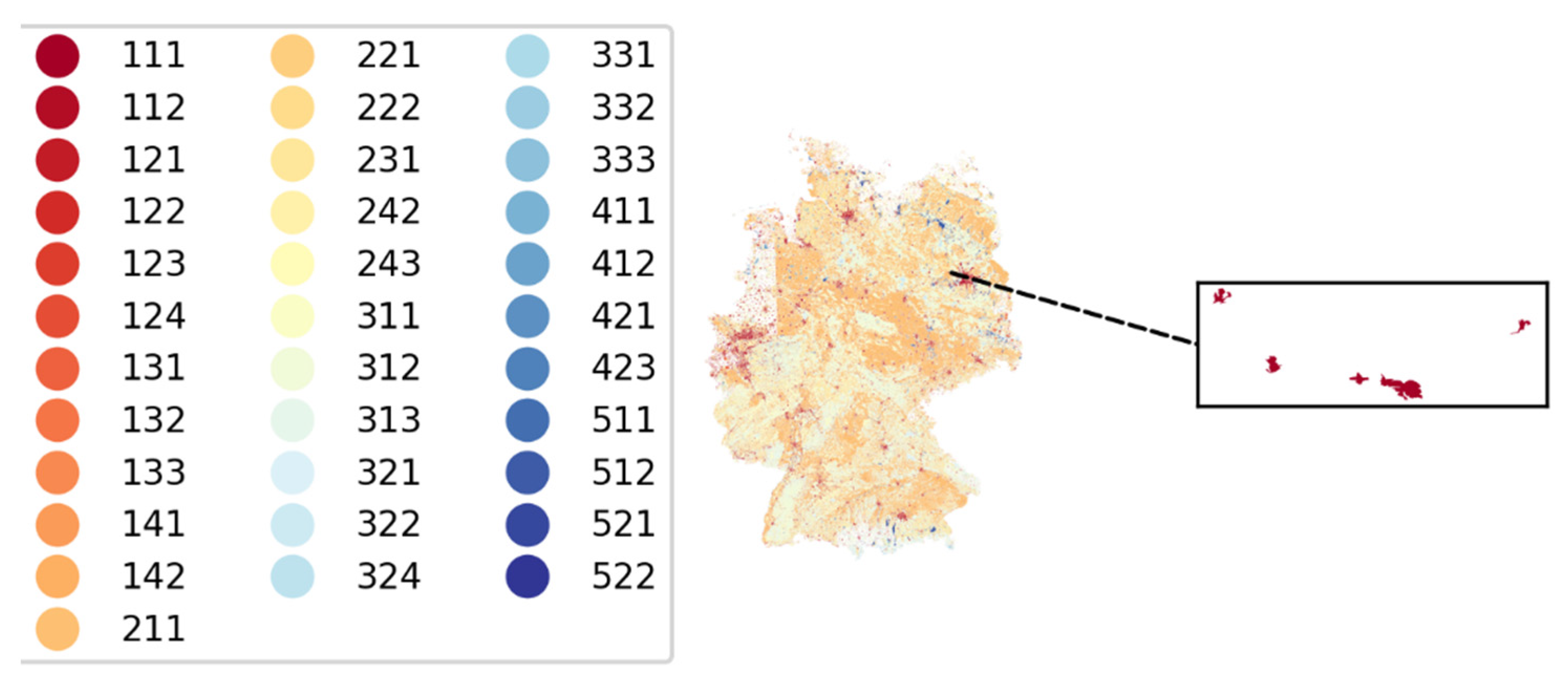
• code 18 (numerical): this feature corresponds to the land cover type (e.g., 111: Continuous urban fabric, 112: Discontinuous urban fabric, 121: Industrial or commercial units, 141: Green urban areas, etc.)

Moreover, a few other features from the most crucial dataset (the 2011 census) were integrated into the OSM buildings data. The dataset for Germany was accumulated across 100 m × 100 m grid cells, as follows:

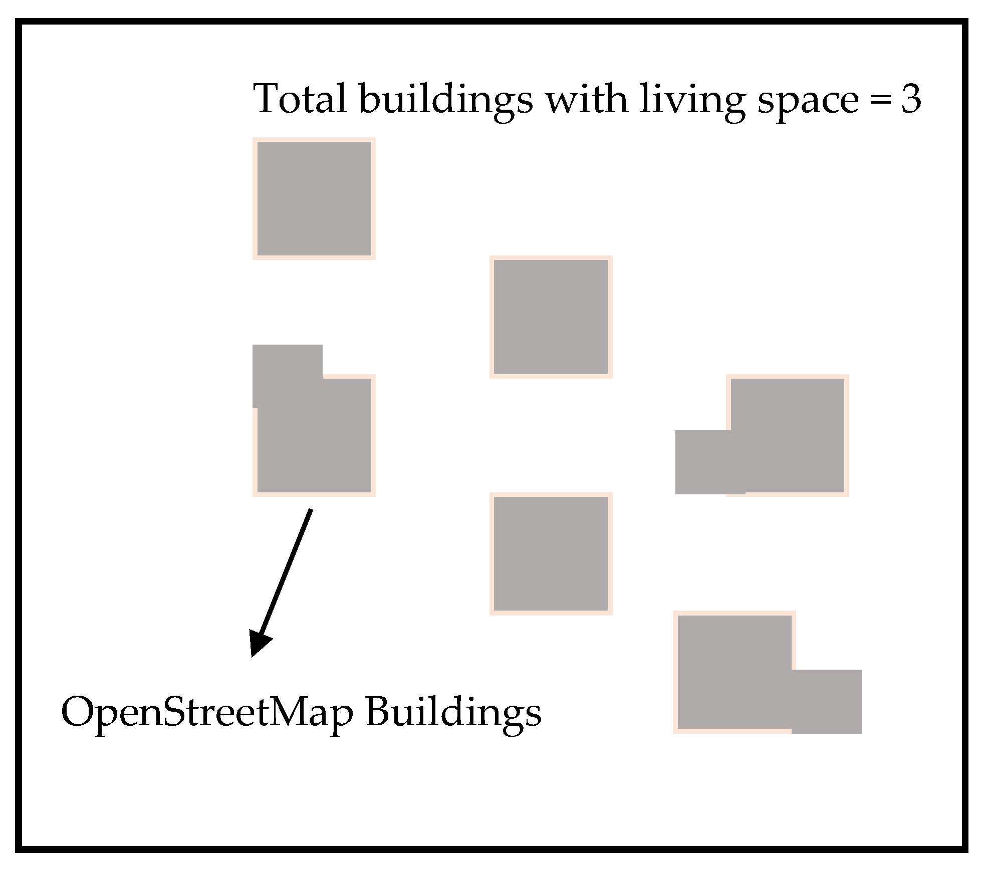
• buildings_living_total (numerical): total number of buildings with living space within a 100 m × 100 m cell.
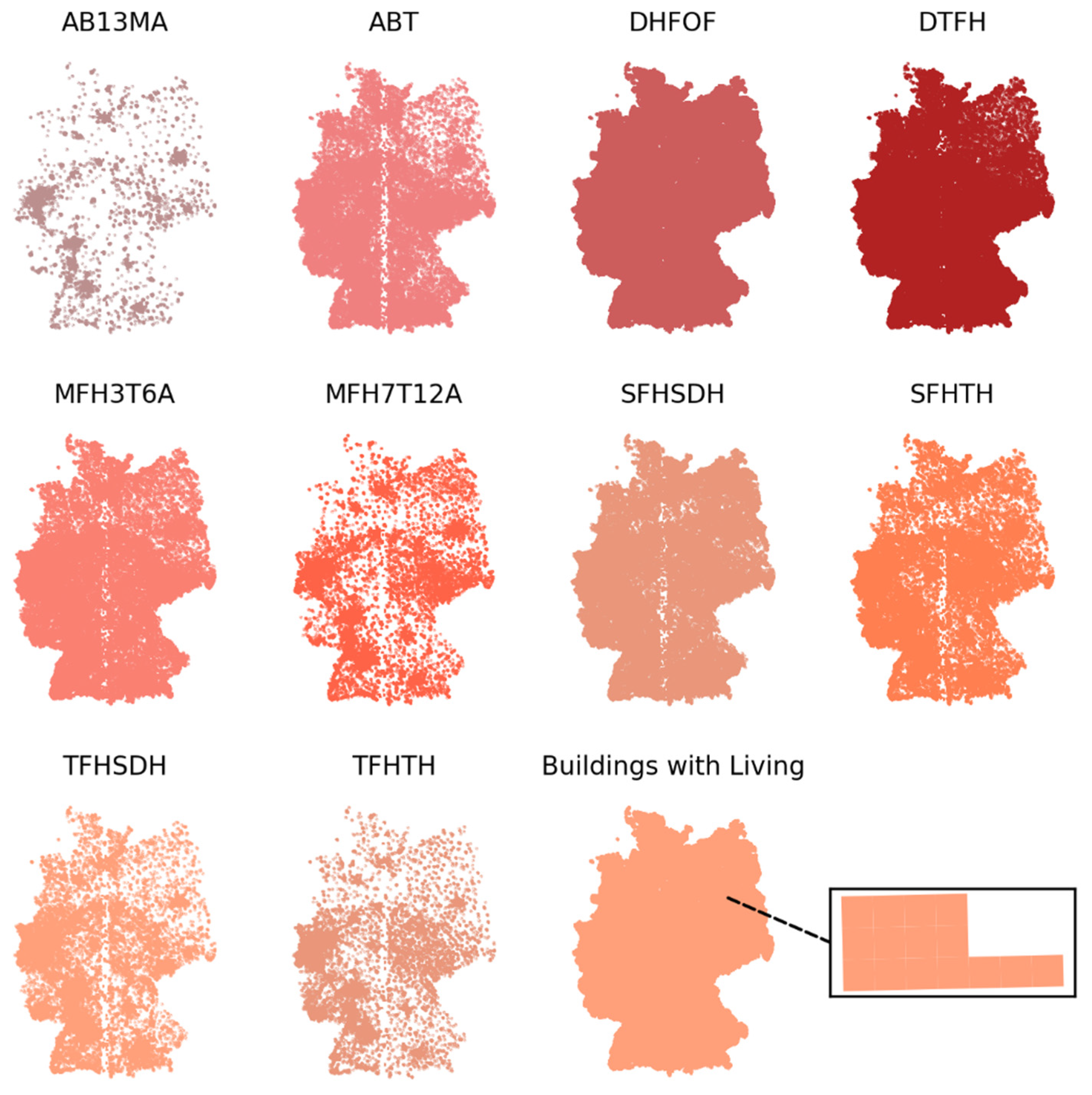
• AB13MA_total (numerical): total number of apartment buildings, with 13 or more within a grid cell.
• ABT_total (numerical): total number of other buildings within a grid cell.
• DHFOF_total (numerical): total number of detached houses for single families within a grid cell.
• DTFH_total (numerical): total number of detached two-family houses within a grid cell.
• MFH3T6A_total (numerical): total number of multi-family houses within a grid cell (3–6 apartments).
• MFH7T12A_total (numerical): total number of multi-family houses within a grid cell (7–12 apartments).
• SFHSDH_total (numerical): total number of single-family houses within a grid cell (semi-detached house).
• SFHTH_total (numerical): total number of single-family houses within a grid cell (terraced house).
• TFHSDH_total (numerical): total number of two-family houses within a grid cell (semi-detached house).
• TFHTH_total (numerical): total number of two-family houses within a grid cell (terraced house).

With the help of these 11 features from the census data, 11 other features were added to each building; see Section 3. These features correspond to a percentage probability of buildings likely to correspond to the given type (i.e., building with living space, apartment, single-family house, multi-family house, and two-family house). These 11 features are percentage_buildings_living, percentage_AB13MA, percentage_ABT, percentage_DHFOF, percentage_DTFH, percentage_MFH3T6A, percentage_MFH7T12A, percentage_SFHSDH, percentage_SFHTH, percentage_DTFH, percentage_SFHTH, all of which constitute integers in percentages.

Finally, the essential characteristics result from the tags from OSM and machine the learning model’s output.

• building_class (categorical): building type labels taken from OSM and labels generated by the machine learning model.
• house_type (categorical): house type labels taken from OSM and labels generated by the machine learning model.

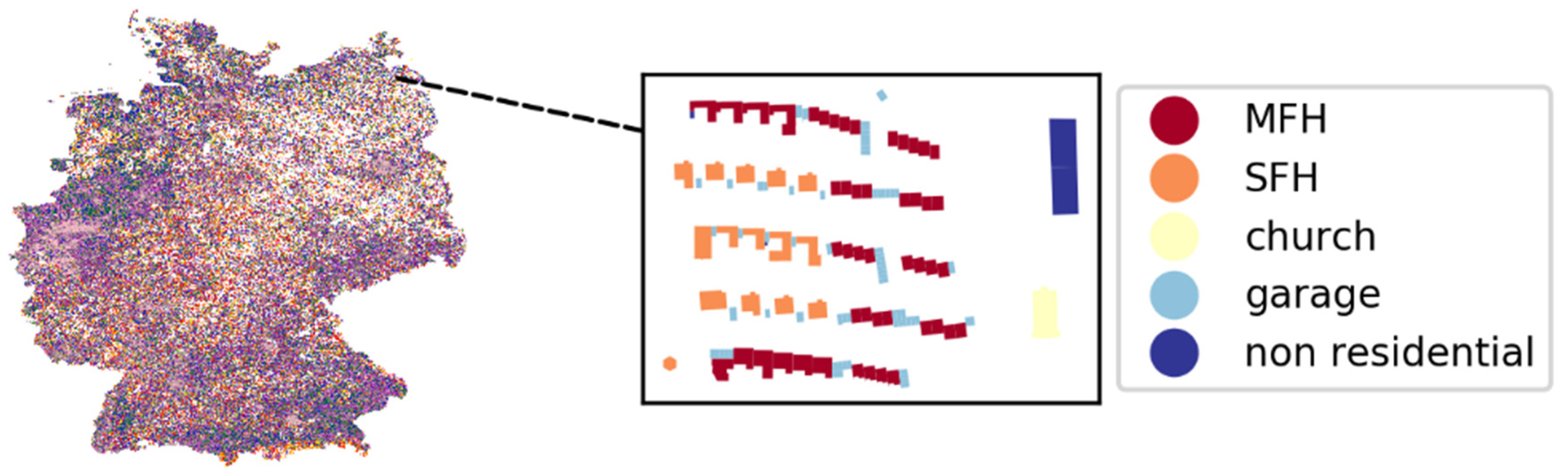
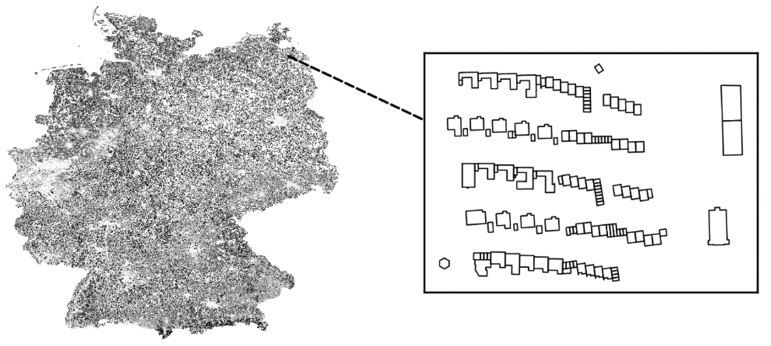
This dataset thus contains 29,497,772 buildings as rows and 32 features for each of the buildings as columns. Figure 1 shows the building footprints and final labels for each unit (zoomed).

3. Methods

After discussing the research gap and the requirement of classifying building types using open data in the introduction section, this section discusses the process of data generation and of extracting and preparing various data elements for the development of a machine learning model. The steps involved in data generation incorporate data extraction from various sources, including the identification of required features, data preprocessing, preparation for training the machine learning model, machine learning model development, prediction of building labels using the model, and technical validation. The steps involved in generating building labels are schematically displayed in Figure 2.

3.1. Data Acquisition

The acquisition of data is the initial phase in the model development process. Data acquisition for various datasets required in preparing the final data is outlined in this subsection. Here, the process involved in collecting the datasets, preprocessing them if necessary, and the file format in which the file was saved, are presented.

3.1.1. OpenStreetMap Data

The first and main dataset used in the modeling was that of the OSM buildings dataset. The OSM data is being investigated as an alternative to remote sensing and POI data. The OSM full metadata, however, is only available to its contributors. Therefore, Geofabrik’s server was used to download it. The server holds data extracts from the OSM project, and the data are updated regularly. For the modeling itself, the most recent data was downloaded from this server [43]. Moreover, the data downloaded contain map components that were redundant for this purpose. For this reason, osmosis [44], a command-line Java application, was used for the OSM data processing. A command-line query that accepts nodes and ways tagged as buildings was provided in the application to extract buildings and their components. The extracted file was in Protocolbuffer Binary Format (PBF). However, this file format is not helpful for modeling purposes, especially in this case, where the data are placed in machine learning algorithms. Hence, data were transferred to the PostgreSQL server using osm2pgsql [45]. From there, the data were extracted to the local disk in the comma-separated values (CSV) format. However, these data feature geographical components and were converted into the Geographical Information Systems (GIS) support format. The coordinate reference system that OSM data have and used while creating the geometries was WGS 84 (i.e., EPSG:3857). Figure 3 shows the building footprints extracted following this approach.

This dataset contains 29,497,772 buildings and 71 features of each of these. However, all of these features are superfluous and hold numerous missing values. Consequently, few essential features are considered from among those available. Therefore, some of the redundant features are removed, reducing the total to 12. The feature considered to represent the building types was named ‘building_type’ and contains various labels. The most essential of these and the labels with the majority of buildings are displayed in Figure 4. However, not every building in the dataset is represented by its type. As Figure 4 shows, the majority of the buildings are tagged as ‘yes,’ representing buildings of unknown type. In addition, the buildings that are labeled with ‘yes’ must be predicted using machine learning techniques. Machine learning model training must be performed on buildings with certain labels. However, the features contain missing values, excluding the building_type feature, which is inadequate for classification. Therefore, this study considers other features from different datasets.

3.1.2. Building Height Data

As previously stated, the characteristics of buildings from the OSM data alone are insufficient for predicting building types; additional features must be added to increase the dataset quality. One useful dataset is that for building height [42], which is one of the key parameters for classifying building types. Obtaining heights for each building is impossible, and no such dataset is available for whole nation. Nevertheless, the urban atlas from the Copernicus project [42] specifies building heights for some major cities. In Germany, the building height dataset for the state of Berlin is available and was downloaded from the urban atlas database [42]. The dataset contains a 10 m high-resolution raster layer with building height information. Moreover, the coordinate reference system this dataset uses is ETR89 (i.e., EPSG:3035). Figure 5 exhibits the raster layers with building height information for the state of Berlin, Germany. Furthermore, the inter-quartile range for the heights ranges from 4 to 14 m (see Figure 5).

3.1.3. CORINE Land Cover Data

Aside from building properties from OSM and building heights datasets, land use data (i.e., continuous urban fabric, discontinuous urban fabric, industrial, commercial, etc.) also add value to the building dataset. This information is available via CORINE land cover datasets produced through the Copernicus project [41]. This dataset is based on the classification of satellite images developed by a team from EEA member countries (i.e., EEA39) [41] and has one feature with 44 classes. The classes in the dataset represent continuous urban fabric, discontinuous urban fabric, industrial or commercial units, and airports; see [41]. As it is considered to be an essential additional feature that adds value to the primary dataset, the dataset was downloaded from the Copernicus land monitoring service [41]. Moreover, the projected coordinate system was ETR89 (i.e., EPSG:3035). Figure 6 displays a geographical representation of the downloaded data. In addition,

Table 1. CORINE land cover code representation.

Code	Representation	Code	Representation
111	Continuous urban fabric	112	Discontinuous urban fabric
121	Industrial or commercial units	122	Road and rail networks and associated land
123	Port areas	124	Airports
131	Mineral extraction sites	132	Dump sites
133	Construction sites	141	Green urban areas
142	Sport and leisure facilities	211	Non-irrigated arable land
212	Permanently irrigated land	213	Rice fields
221	Vineyards	222	Fruit trees and berry plantations
223	Olive groves	231	Pastures
241	Annual crops associated with permanent crops	242	Complex cultivation patterns
243	Land principally occupied by agriculture	311	Broad-leaved forest
312	Coniferous forest	313	Mixed forest
321	Natural grasslands	322	Moors and heathland
323	Sclerophyllous vegetation	324	Transitional woodland-shrub
331	Beaches, dunes, sands	332	Bare rocks
333	Sparsely vegetated areas	334	Burnt areas
335	Glaciers and perpetual snow	411	Inland marshes
412	Peat bogs

provides the code representation of CORINE land cover data.

3.1.4. Census Data

In addition to the above-mentioned datasets, census data for Germany was considered. In 2011, a register-based census survey was conducted in Germany. This survey was conducted to determine how many people live and work in Germany, and how they do so. In addition, the census data was extended in the area of buildings and apartments to include the total number of buildings with living spaces, types of apartments, form of ownership, number of apartments in the building, and type of heating, with a resolution down to the municipality level [3]. Comprehensive data regarding buildings and apartments were downloaded from the 2011 census database [3]. This dataset corresponds to the total number of buildings with living spaces per 100 m × 100 m grid cells. The data were further split into different types, namely: single-family houses, two-family houses, multi-family houses, and apartment buildings.

Furthermore, each grid cell in the dataset was assigned a unique identity that was further combined with the geographical shapefile corresponding to each cell. The geographical shapefile was download from the Geoinformation and Geodesy databases [46]. The data also included a unique ID like that of previously-downloaded building and apartment data. With the help of these unique IDs, geographical shapefiles were added to each grid cell, thus forming a complete georeferenced dataset for each building type. Moreover, this dataset’s projected coordinate reference system is similar to the CORINE data (i.e., EPSG:3035). Figure 7 indicates the locations of the grid cells and the total number of units for each type for Germany. Additionally,

Table 2. Total number of buildings per building type in Germany.

Feature	Abbreviation	Count
buildings_living_total	Buildings with living space	18,494,939
DHFOF	Detached house for one family	1,637,974
SFHSDH	Single-family house: semi-detached	411,851
SFHTH	Single-family house: terraced	292,062
DTFH	Detached two-family houses	552,705
TFHSDH	Two-family house: semi-detached	65,266
TFHTH	Two-family house: terraced	50,873
MFH3T6A	Multi-family house: 3–6 dwellings	437,990
MFH7T12A	Multi-family house: 7–12 dwellings	153,802
AB13MA	Apartment building: 13 or more units	36,214
ABT	Another building type	104,205

presents the total number of buildings according to their type. Here, a detached house is considered a free-standing building; irrespective of its type, a semi-detached house is a building that is built against another building, a terraced house is a building that is built against two other buildings, and other building types are those which are not a detached house, semi-detached house, or terrace house, and encompass all types of inhabited domiciles.

3.2. Data Preprocessing

Having discussed the datasets for modeling, this section introduces data preparation. In this stage, all of the features from the above-mentioned datasets were added to the OSM building dataset. In order to combine all of the datasets, the coordinate reference system for each one should be the same. For convenience, a coordinate reference system WGS 84 (i.e., EPSG:3857) was selected because the primary (i.e., OSM) data were placed in this reference system, and all of the datasets were projected to this coordinate system.

First, the CORINE land cover data feature was added to the OSM buildings by intersecting the buildings with the CORINE data. Performing this task provided an additional feature with land cover information for each building. Next, the building height information for the buildings in Berlin was added by intersecting the buildings with the building height information dataset, which delivered building height features for the buildings in the city. Furthermore, buildings outside the state were assigned null values and considered missing values for the purposes of this feature. Finally, census data with 11 features shown in Table 2 were assigned to the dataset. Following this operation, the final data contained 29,497,772 buildings with 19 features for each building. However, several values were missing for each feature, which will be addressed in the following subsection.

After combining the features from various sources with the final dataset, further processing was performed on the target class (i.e., building_type). As can be seen from Figure 4, there were several uncertainties in the tags within the OSM dataset. There were almost 1575 unique tags in this feature (i.e., building_type). The cause of this uncertainty was the ambiguous representation of the buildings, e.g., spelling errors, multi-language use, etc. Nevertheless, some of these uncertainties are presented in

Table 3. Ambiguity of data labels/tags in the target class.

Building	Varying Representation
Apartments	Apartments|Apartment building
Warehouse	Lagerhaus|Lagerhalle
Terrace	Terrasse
Youth Centre	Jugendzentrum
Nursing home	Plegeheim
House	Haus|Hause|house

.

However, refinement of these features reduced the labels to 895 unique types, which is still a large number. Therefore, the labels in the target class were further reduced to 25 based on a Wiki model [47] and named ‘building_class’, which now constitutes the target class for classification.

Furthermore, many buildings are evidently not suitable for living in—for instance, garages, which are considered buildings and labeled as ‘yes’ (i.e., buildings of unknown type) in the OSM dataset. Additionally, the built-up area for garages varies according to individual requirements, but most garages were built to typical size specifications. From pre-labeled buildings, the area of the building types with garages/attachments is shown in Figure 8. From the figure, it can be seen that around 75% of buildings with areas of fewer than 35 m² were labeled garages/attachments. Hence, using this information, buildings with a size less than or equal to 35 m² were labeled as garages in the target class.

Additionally, information from census dataset features and new features representing percentage probabilities for each building were generated. These new features were formulated by applying the fraction of the total number of buildings with living space from the census data per grid cell to the total number of OSM buildings in that specific grid cell (for clearer understanding, see Figure 9). Figure 9 shows the total number of buildings with living space from the census dataset for this 100 m × 100 m grid cell, which is three. In addition, a total of six OSM buildings are in this cell. Therefore, each building in the grid has a 50% chance of being a residential building/building with living space. By applying this procedure to other features extracted from the census dataset (refer to Table 2), 11 new features with percentage probabilities for each building type were generated.

Now, using this information, buildings with 100% or more changes to become a building with living space were labeled in the target class as residential. After applying all of these preprocessing steps, the dataset contained 29,497,772 buildings with 30 features.

3.3. Data Analysis

In addition to the preprocessing of the data, the dataset was further analyzed to address challenges with respect to the data itself. Prior to this step, the buildings with labels in the target class numbered 6,047,266, which amounted to 20.41% of the total buildings. However, after preprocessing, the labeled data in the target class were increased to 35.12% of the total buildings. Moreover, increasing the labels in the target class helps achieve more efficient model performance. Figure 10 displays the labeled buildings before and after preprocessing. The labeled data following preprocessing was used for training the machine learning model. In addition, the prediction was performed on the unlabeled data using the trained model.

However, further analysis of the data indicators reveals that 77% of the values in the dataset were missing. Nevertheless, the lack of data per feature is shown in Figure 11. There were 0% missing values in the feature containing the building identification numbers and area of each. However, there were missing values in the other features, which led to inefficient model performance. Therefore, it is necessary to fill in the missing values for each feature. The missing data can be filled by using specific techniques, which are discussed in the next subsection.

Analyzing the distribution of each label in the target class presented a problem of class imbalance in the dataset. Figure 12 displays the distribution of labels in the target class. Most of these were attachments, residential, commercial, industrial, and agricultural, at 52.81%, 35.29%, 9.02%, 0.57%, and 0.98%, respectively. This means that attachments and residential units shared the highest percentage at 88.10%, and the remaining labels only constituted 11.90%. Therefore, if the model is trained on this dataset, the algorithm has a higher chance of picking up the label with more weight in the dataset.

To conclude, after analyzing it, the dataset presented problems in terms of missing values and class imbalances. Nevertheless, these challenges are addressed by adopting a classification with the missing values and class imbalance.

3.4. Classification

The classification task is the next crucial stage in the model generation process once the data has been prepared. This section provides details about the adopted machine learning models and the experiments conducted on the dataset. The dataset with the known labels was considered for training the machine learning models. In the classification process, a two-step approach was used to classify the building types. For the first task, classification was performed in order to classify residential and non-residential buildings. In the second, classification was performed to classify houses (i.e., single-family houses, multi-family houses, and apartments) among the predicted residential buildings. Figure 13 shows the methodology adopted for the building type classification.

Upon analyzing the dataset presented in the previous subsection, it was found to suffer from two main issues, namely missing values and class imbalance. In order to overcome these challenges, two different methods were considered. These methods included implicit and explicit approaches. In the implicit method, missing values, class imbalance, and classification tasks were solved within a single architecture. Here, two models were deployed: HexaGAN [48] and a modified Artificial Neural Network (ANN) [49]. In addition, the explicit method, including missing value imputation, class imbalance, and classification tasks, was performed using different models consecutively. Multiple Imputation by Chained Equations (MICE) [50] was used to resolve the missing value problem in the first step. By applying MICE, the missing values in the training dataset could be filled with model-generated ones. In order to generate balanced labels in the target class, Synthetic Minority Oversample Techniques (SMOTE) [51] and cost-sensitive learning for imbalance classification (Class-Weighting) (CS) were considered. This model was then applied to the training dataset to produce balanced labels by overcoming class imbalance issues. Finally, the classification problem was solved by means of a Random Forest classifier.

3.4.1. Experiments

Using the model’s setup, experiments were conducted on the training dataset. Three state-of-the-art machine learning algorithms for classification with missing values and class imbalance (both implicit and explicit) were tested. However, the best-performing algorithm was used as the final model in order to perform the building type classification task. The classification performances of three models were tested on the training dataset. Here, implicit algorithms were implemented, trained and tested with baseline data and compared to the baseline results. Furthermore, all of the models were trained with the preprocessed training dataset. In this context, all of the experiments were repeated ten times with five-fold cross-validation. In order to evaluate the model performance, F1 score metrics were used and calculated for all three of the models.

Table 4. Classification performance of the models.

Model	Baseline Results	Implementation with Baseline Data	OSM Data
HexaGAN(Implicit Model)	0.9762 ± 0.021	0.9780	0.8154
Modified ANN (Implicit Model)	0.8170	0.7911	0.6308
Explicit Model	-	-	0.9958

displays the performance of the considered models.

From the results obtained with the respective algorithms using the OSM data, the model with MICE, CS, and a random forest classifier performed far better than the other models. Nevertheless, the other two models are unique in their methodologies and performed impressively on the baseline datasets. However, the explicit method outperformed the two implicit ones using the OSM data. Therefore, to predict the missing building types, the explicit method; MICE, together with class-weighting and a random forest classifier model were chosen.

The building type labels were predicted with the selected model. The results for the predicted building types were as shown in

Table 5. Building type classification results for buildings in Germany.

Building Type	Predicted Count
Residential	19,747,802
Attachments	5,583,658
Commercial	3,127,442
Industrial	460,698
Hospital	217,103
Hotel	114,013
Agricultural	105,888
Government	151,98
Event venues	35,935
School	46,452
Religious	33,645
Transport	3117
University	2927
Military	1048
Others	2866

. The major labels predicted were residential, attachments, commercial, and industrial. However, the share of residential labels was greater when compared to all others. Using the predicted labels, all labels other than the residential were considered as non-residential buildings. The total of 19,747,802 residential buildings were further utilized to classify house types (i.e., single-family, multi-family, and apartments).

The second task in these two folded approaches was to classify residential buildings into house types. The training data for the model consisted of label data from the residential buildings predicted in the previous step. In addition, the target class for this classification was the new feature class drawn from the ‘building_type’ feature and named as the ‘house type.’ However, less than 2% of data with proper house types was labeled in the OSM data. Moreover, the labels therein differed from those expected; see

Table 6. House type labeling.

OSM Building Type	Proposed House Type
Detached	Single-Family House
Semi-Detached	Multi-Family House
Terrace	Multi-Family House
Apartment	Apartment
House	To predict
Residential	To predict

. With the aid of this, the dataset was labeled according to the proposed types listed in Table 6. These assumptions were considered to increase the quality, as well as to match with the expected house. Furthermore, in order to increase the training data, the same procedure used in the preprocessing step to pre-label residential buildings with the help of percentage probability features was applied here. If the percentage probability of building type is greater than or equal to 100%, the buildings are labeled according to their respective house type. Furthermore, as per Table 2, different single-family, two-family, and multi-family houses were combined into single-family and multi-family houses.

The target class label distribution, showing the class imbalance proportion after preprocessing of the data, is shown in

Table 7. Distribution of house type target class.

Class	Count	Percentage
Single-Family House	1,063,379	60.07%
Multi-Family House	386,995	21.86%
Apartment	319,663	18.06%

. Here, the single-family house shares a large portion compared to the other two labels. The class imbalance issue addressed in the previous subsection helps overcome this issue when modeling.

An experiment using the best model assumption considered in the first task was adopted with this final data. The model with MICE, together with oversampled SMOTE and weighted data, was trained on 1,769,997 samples. The rest of the 17,977,805 residential buildings were predicted with the help of this model. The total house types, following prediction of the residential buildings in Germany, are shown in

Table 8. House type for residential buildings in Germany.

Class	Count
Single-family House	14,378,635
Multi-Family House	4,350,183
Apartment	1,018,984

. The predicted results reflect the fact that the majority of the buildings are single-family houses.

3.4.2. Technical Validation

This section validates the findings after generating the dataset with labels for each building footprint with residential, non-residential, single-family house, multi-family house, apartment building, industry, commercial, and so on. There is no ground truth to be used to evaluate the data outcomes of the model. However, our primary concern was to label all of the buildings extracted from OSM as residential and non-residential. In addition, the residential buildings were to be classified into different house types. Validation of the predicted building labels was performed using the census data. The total number of residential buildings in Germany was 19,053,216 [52]. However, the total predicted residential buildings amounted to 19,747,802, with a percentage error of 3.64%. This means that the model predicted 3.64% more buildings as residential of the total residential buildings in Germany. Figure 14 shows a comparison of the total residential buildings in Germany and the predicted ones.

Furthermore, in order to spatially verify the quality of the predicted buildings, validation was performed using the census data for each federal state in Germany. Figure 15 displays the predicted residential building count per federal state and the corresponding information according to the official data for that state. The percentage error for the predicted residential buildings in each state ranged from a minimum of −18.68% to a maximum of 22.73%. The results clearly indicate that the predicted residential buildings for the two states of Baden-Württemberg and North Rhine-Westphalia are comparatively more than other states. This may be because these states feature more buildings compared to other ones. Moreover, the buildings taken from these states for training were fewer, which could be a possible reason for the percentage error.

Figure 16 shows the correlation between the predicted residential buildings and the actual, which is close to one. However, more training data with proper labels and fewer missing values could improve the percentage error.

Further validation of the predicted data for house type was performed using the official statistics. The total single-family houses in Germany numbered 12,707,978, with predicted single-family houses totaling 14,378,638, with a percentage error of 13.14%. Furthermore, multi-family houses and apartments were considered multi-family houses because the statistical data contained two-family houses that were not considered while predicting house types. Nevertheless, the total number of multi-family houses, including two-family and multi-family ones, as well as residential establishments, was 6,345,238. Meanwhile, predicted multi-family houses and apartments totaled 5,369,167. Upon comparing the real data with the predicted data, a percentage error of −15.38% was noted, as shown in Figure 17.

Further spatial validation was performed by accumulating the single-family house stocks for federal states and comparing this with the data for each federal state. Figure 18 shows predicted single-family houses in each federal state and a comparison with the statistical data. The percentage error for the predicted single-family houses ranged from a minimum of −16.59% to a maximum of 50.88%. The maximum errors were recorded for the three states of Baden-Württemberg, North Rhine-Westphalia, and Sachsen, with 37.63%, 38.38%, and 50.88%, respectively. The large deviation in the prediction count was due to the unavailability of the actual required labels in the OSM data. Furthermore, this task was solely dependent on the assumption and predefined labeling of the target class with the help of census data. Therefore, an improvement in the actual required labeling in the OSM data could overcome these challenges in the future.

Nevertheless, by all standards this is a good sign, as it was, to the best of our knowledge the first time that the building types obtained from OSM data were classified in their entirety for Germany.

4. Discussion

Building type information serves as the foundation for a variety of models, including energy, mobility, disaster management, health care, and other applications that benefit humanity in a variety of ways. For example, in energy system models, forecasting the future energy required at the national level requires knowledge of the type of building and how it will be used. In the end, the introduction of environmentally friendly technologies is aided by this prognosis. Furthermore, this is not just in the energy systems, as ref. [33] employed building types to locate buildings where pesticide spraying was necessary, demonstrating that building level information is significant in the health sector. Therefore, information at the building level is essential for technological and economic advancements.

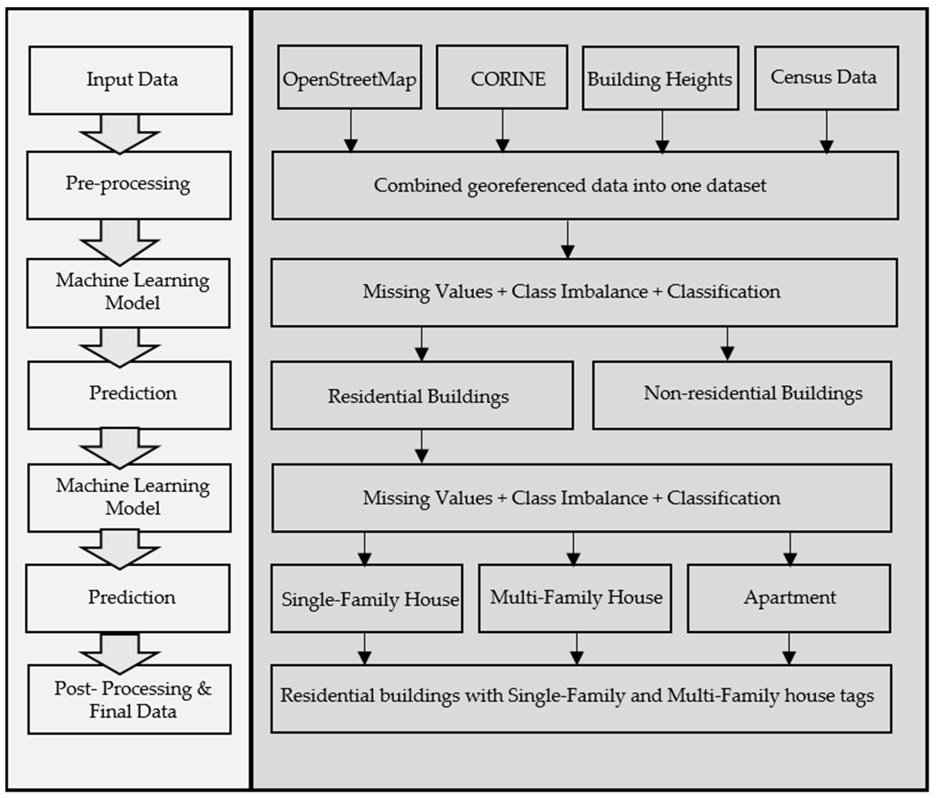
To identify building types, earlier research relied primarily on remote sensing data, geospatial vector data, and POI data from government agencies, mapping agencies, commercial POI data suppliers, and real estate cadasters, among others, despite data availability and computational complexity limitations. This study establishes the building type classification for the entire country by addressing the above limitations and resolving missing values and class imbalances in OpenStreetMap POI data and by mapping additional data to increase classification accuracy. Apart from OSM data with building footprint geometries and POI data, other data such as land cover data, census details, and building height data were also mapped to the building footprints in this study. However, the following are some of the advantages of the suggested classification methodology: To begin, the building footprints and POI data are derived directly from the same source of data, whereas in previous studies, the building footprints and POI data were derived from independent sources; as a result, mapping POI data to the building footprint is not always reliable. Second, the extra data from the census (manually surveyed) is mapped to the country’s existing dataset. Besides census data, land cover data with several classes has also been mapped in order to increase the accuracy of the classification. Third, the missing values and class imbalance concerns in the OSM data were handled by using implicit and explicit methods of classification algorithms that account for missing values and class imbalance issues. However, when trained on OSM labeled data, the explicit method outperforms the implicit methods.

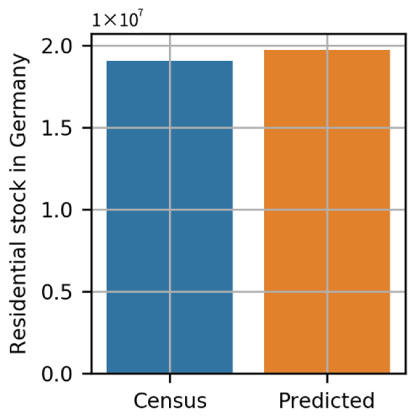
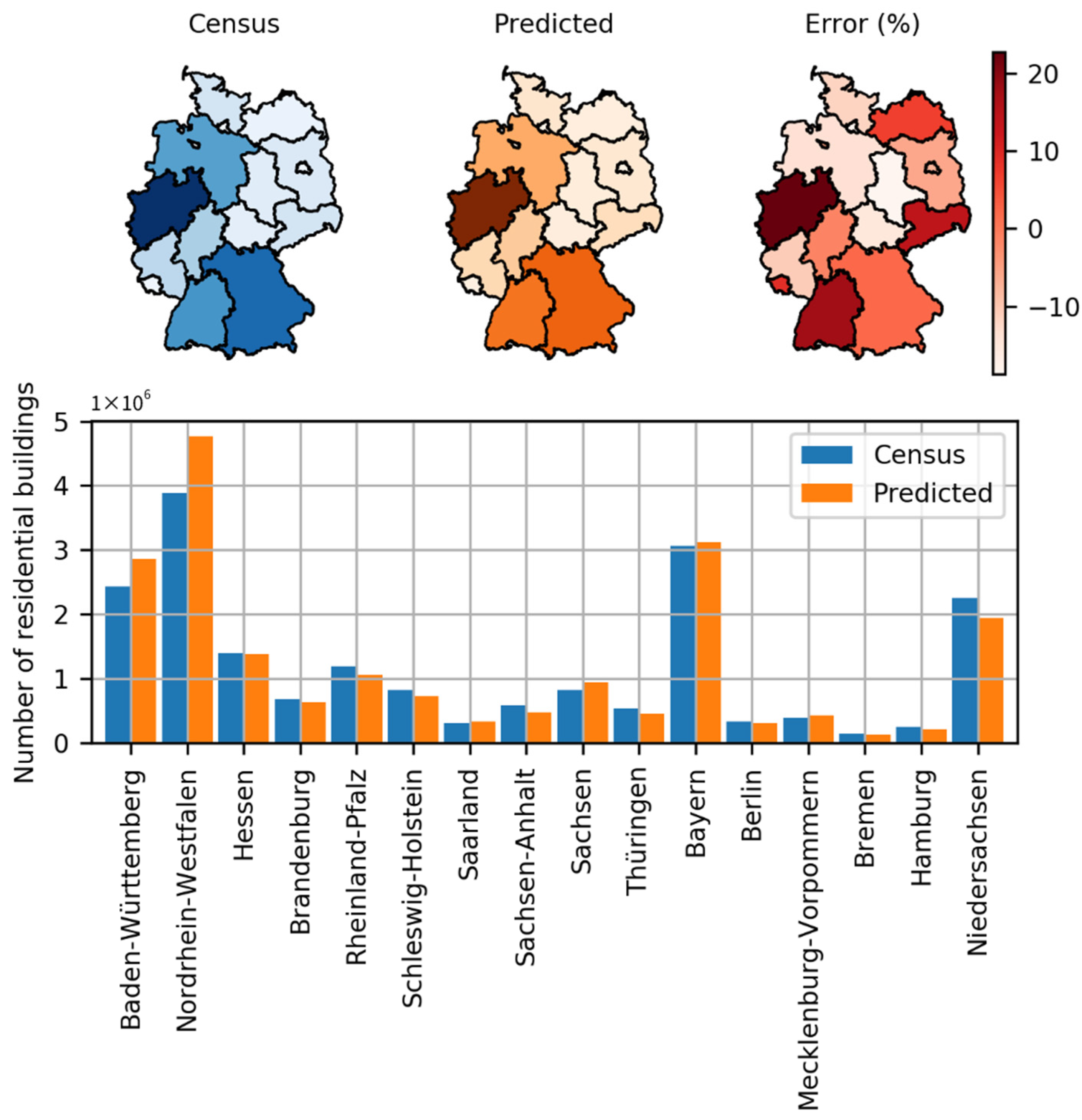
When deployed, the explicit method classified approximately 29 million building footprints into approximately 19 million buildings and the remainder as non-residential buildings, which comprised industrial, commercial, garage, and noncommercial-nonindustrial buildings. When compared to official statistics, the results indicate a percentage error of 3.64%. Furthermore, when compared to [23], these results are encouraging, since ref. [23] classifies polygons extracted from a real estate cadaster as residential buildings with a percentage error of 4.9% for Germany. Additionally, ref. 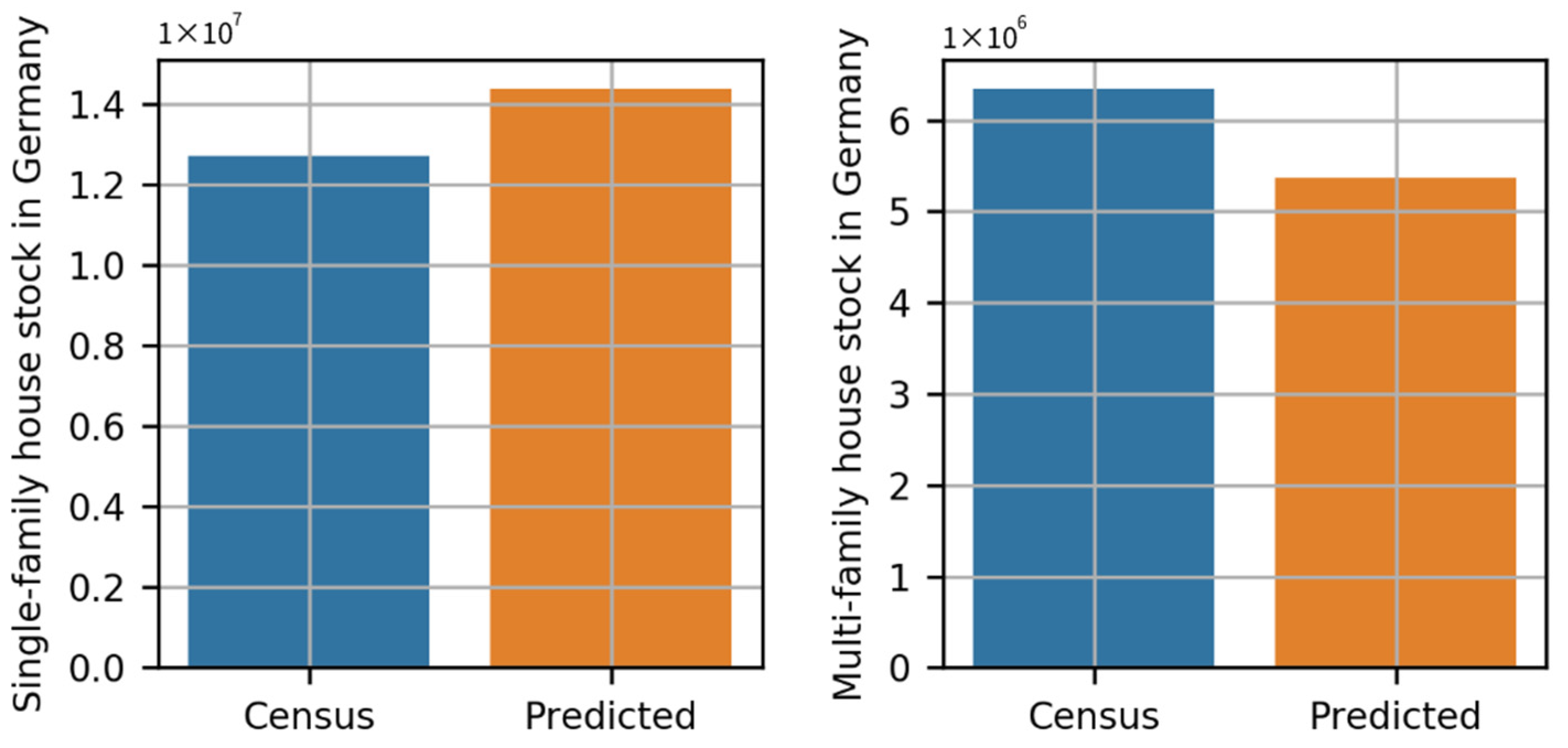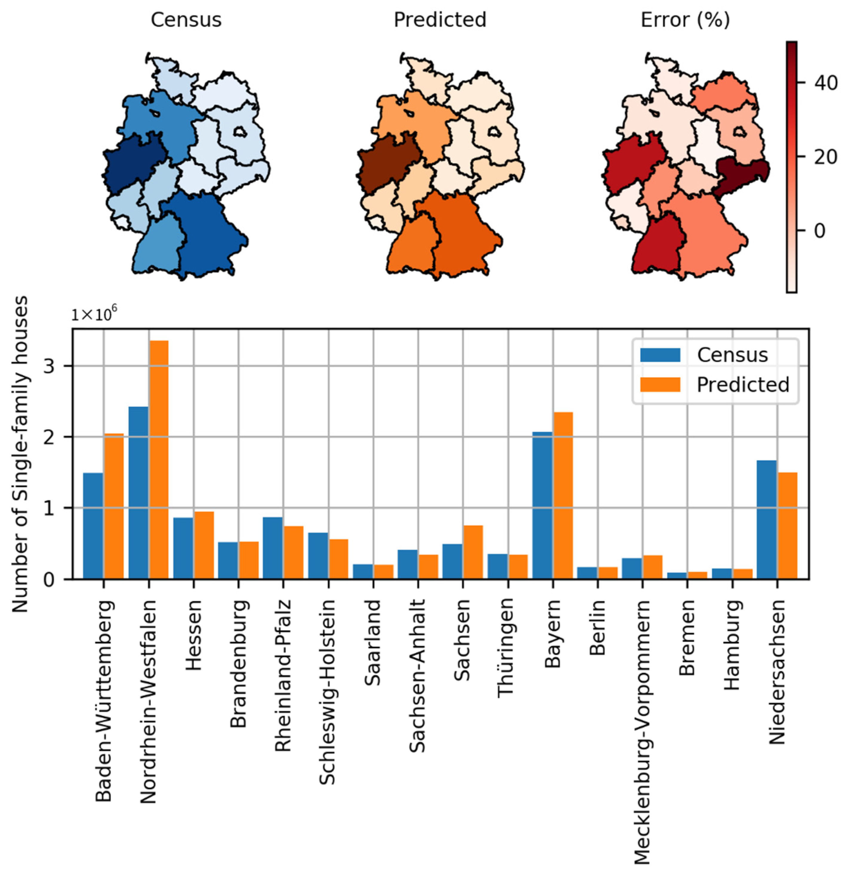[23] recommends using OSM data as supplemental data for classification. On the other hand, our study utilized OSM data and classified building types by addressing challenges with the OSM dataset (i.e., missing values and class imbalance). Furthermore, our analysis identified each residential building as a single-family house, a multi-family house, or an apartment building with a percentage error of 13.14% and −15.38%, respectively.

The collected results, however, are applied to the energy system model. Geo-referenced synthetic electrical distribution networks for Germany are estimated using data corresponding to residential buildings. Before the tagged residential building data for Germany was included in this model, the geo-referenced synthetic electrical low-voltage distribution networks developed had a percentage error of 33% when validated against the overall low-voltage network length for Germany [53]. However, when classified residential buildings are included in the geo-referenced synthetic distribution network generator model, a percentage error of 0.89% is obtained. This improvement in the energy system model’s percentage error reflects the building type classification model’s accuracy. However, its accuracy varies depending on the model, as this model considers the entire nation, and any mismatch in one geographical location may be compensated for in another. As a consequence, it can be stated that the method employed delivered superior results and addressed the gap created by the complex image classification and POI data availability.

However, according to the findings of this study, the data mapping to the OSM data is still inadequate for the classification of non-residential buildings. The census data employed to achieve the precise classification concentrated exclusively on residential buildings and population. Additionally, the land cover data label the polygons to indicate if they are in an industrial or non-residential zone. Thus, additional data that assists in training the model that can focus on identifying the precise commercial and industrial buildings (i.e., offices, restaurants, supermarkets, glass industries, hospitals, schools, mini-supermarkets, shopping complex, etc.) provides additional classification of non-residential buildings. Moreover, this study covers a single nation owing to the requirement of developing a model capable of generating geo-referenced synthetic electrical distribution networks. Nevertheless, with certain adjustments, this methodology may be extended to other nations. The constraints may occur during the pre-processing stage due to ambiguity in the labels due to spelling errors and multilingual use. The manual decision tree recognizes and updates the labels based on the data analysis conducted on the building labels. If the uncertainty is due to the language, a different approach would be necessary in this stage when applying this methodology to another nation. This is because OSM maps are entirely volunteer based, and if an individual contributor does not adhere to the process for labeling, the labels will be ambiguous. This limitation will prevent this methodology from being used in other countries; however, with some data analysis and adaptive labeling during the preprocessing stage, this limitation can be addressed.

5. Conclusions

The dataset was developed by classifying building types extracted from OSM data for Germany with the specific goal of generating geo-referenced synthetic electrical distribution networks and assessing synthetic energy profiles for the buildings. However, this dataset can be used in any other models that require building information.

Our approach consists of classifying building types with missing values and class imbalances in data extracted from OSM, from which the primary building data were drawn. This study also considered different datasets from various sources and added these to the primary dataset. Moreover, careful refining of the data, including hand label and data cleaning, was performed as part of the data-driven approach. This study employed two state-of-the-art implicit algorithms to classify missing values and class imbalances in one architecture and an explicit cascaded approach. The best performance model was used to classify building and house types in Germany.

The experiments conducted for this study showed the ability to predict building types in light of building footprints and some features corresponding to these. The results indicated a percentage error of 3.64% for the classification of residential buildings, 13.14% for single-family houses, and −15.38% for multi-family houses classification. In addition, this percentage error could be attributed to significant missing values and fewer features. Applying these results to the geo-referenced synthetic distribution model, the percentage error in the total network length was reduced from 33% to 0.89%.

However, given the limitations of non-residential building type prediction and the need to increase the accuracy of house type prediction (i.e., single-family house, multi-family house, and apartment building), some of these points should be considered in future work. First, more data should be collected to avoid misinterpretation of missing values in the dataset. Second, a significant number of additional features with building parameters would contribute to improving the model’s accuracy. Third, more fine-grained location-based data would help in the evaluation of inference data.

References

1. Aubrecht, C.; Steinnocher, K.; Hollaus, M.; Wagner, W. Integrating earth observation and GIScience for high resolution spatial and functional modeling of urban land use. Comput. Environ. Urban Syst. 2009, 33, 15–25. [Google Scholar] [CrossRef]
2. Maantay, J.; Maroko, A. Mapping urban risk: Flood hazards, race, & environmental justice in New York. Appl. Geogr. 2009, 29, 111–124. [Google Scholar] [PubMed] [Green Version]
3. Zensus-2011. Ergebnisse des Zensus 2011 zum Download—Erweitert. Available online: https://www.zensus2011.de/DE/Home/Aktuelles/DemografischeGrunddaten.html?nn=3065474 (accessed on 8 August 2020).
4. Deng, Y.; Chen, R.; Yang, J.; Li, Y.; Jiang, H.; Liao, W.; Sun, M. Identify urban building functions with multisource data: A case study in Guangzhou, China. Int. J. Geogr. Inf. Sci. 2022, 1–26. [Google Scholar] [CrossRef]
5. Huang, Y.; Zhuo, L.; Tao, H.; Shi, Q.; Liu, K. A novel building type classification scheme based on integrated LiDAR and high-resolution images. Remote Sens. 2017, 9, 679. [Google Scholar] [CrossRef] [Green Version]
6. Du, S.; Zhang, F.; Zhang, X. Semantic classification of urban buildings combining VHR image and GIS data: An improved random forest approach. ISPRS J. Photogramm. Remote Sens. 2015, 105, 107–119. [Google Scholar] [CrossRef]
7. Belgiu, M.; Tomljenovic, I.; Lampoltshammer, T.J.; Blaschke, T.; Höfle, B. Ontology-based classification of building types detected from airborne laser scanning data. Remote Sens. 2014, 6, 1347–1366. [Google Scholar] [CrossRef] [Green Version]
8. Duchscherer, S.E. Classifying Building Usages: A Machine Learning Approach on Building Extractions. Master’s Thesis, University of Tennessee, Knoxville, TN, USA, 2018. [Google Scholar]
9. Jochem, W.C.; Leasure, D.R.; Pannell, O.; Chamberlain, H.R.; Jones, P.; Tatem, A.J. Classifying settlement types from multi-scale spatial patterns of building footprints. Environ. Plann. B Urban Anal. City Sci. 2021, 48, 1161–1179. [Google Scholar] [CrossRef]
10. Lin, A.; Sun, X.; Wu, H.; Luo, W.; Wang, D.; Zhong, D.; Wang, Z.; Zhao, L.; Zhu, J. Identifying urban building function by integrating remote sensing imagery and POI data. IEEE J. Sel. Top. Appl. Earth Obs. Remote Sens. 2021, 14, 8864–8875. [Google Scholar] [CrossRef]
11. Dimassi, M.; Samhat, A.E.; Zaraket, M.; Haidar, J.; Shukor, M.; Ghandour, A.J. Buildings Classification using Very High Resolution Satellite Imagery. arXiv 2021, arXiv:2111.14650. [Google Scholar]
12. Wurm, M.; Droin, A.; Stark, T.; Geiß, C.; Sulzer, W.; Taubenböck, H. Deep learning-based generation of building stock data from remote sensing for urban heat demand modeling. ISPRS Int. J. Geo Inf. 2021, 10, 23. [Google Scholar] [CrossRef]
13. Xie, J.; Zhou, J. Classification of urban building type from high spatial resolution remote sensing imagery using extended MRS and soft BP network. IEEE J. Sel. Topics Appl. Earth Obs. Remote Sens. 2017, 10, 3515–3528. [Google Scholar] [CrossRef]
14. Sritarapipat, T.; Takeuchi, W. Building classification in Yangon City, Myanmar using Stereo GeoEye images, Landsat image and night-time light data. Remote Sens. Appl. Soc. Environ. 2017, 6, 46–51. [Google Scholar] [CrossRef]
15. Jochem, W.C.; Tatem, A.J. Tools for mapping multi-scale settlement patterns of building footprints: An introduction to the R package foot. PLoS ONE 2021, 16, e0247535. [Google Scholar] [CrossRef] [PubMed]
16. Yi, Y.; Zhang, Z.; Zhang, W.; Zhang, C.; Li, W.; Zhao, T. Semantic segmentation of urban buildings from VHR remote sensing imagery using a deep convolutional neural network. Remote Sens. 2019, 11, 1774. [Google Scholar] [CrossRef] [Green Version]
17. Zheng, Y.; Weng, Q. Model-driven reconstruction of 3-D buildings using LiDAR data. IEEE Geosci. Remote Sens. Lett. 2015, 12, 1541–1545. [Google Scholar] [CrossRef]
18. Zhu, H.; Cai, L.; Liu, H.; Huang, W. Information extraction of high resolution remote sensing images based on the calculation of optimal segmentation parameters. PLoS ONE 2016, 11, e0158585. [Google Scholar] [CrossRef]
19. Batty, M. Planning support systems: Progress, predictions, and speculations on the shape of things to come; CASA Working Paper Series 122. In Proceedings of the Planning Support Systems for Urban and Regional Analysis, Cambrdige, MA, USA, 27–28 September 2007. [Google Scholar]
20. Lu, Z.; Im, J.; Rhee, J.; Hodgson, M. Building type classification using spatial and landscape attributes derived from LiDAR remote sensing data. Landsc. Urban Plann. 2014, 130, 134–148. [Google Scholar] [CrossRef]
21. Droin, A.; Wurm, M.; Sulzer, W. Semantic labelling of building types. A comparison of two approaches using Random Forest and Deep Learning. Publik. DGPF 2020, 29, 527–538. [Google Scholar]
22. Jochem, W.C.; Bird, T.J.; Tatem, A.J. Identifying residential neighbourhood types from settlement points in a machine learning approach. Comput. Environ. Urban Syst. 2018, 69, 104–113. [Google Scholar] [CrossRef]
23. Hartmann, A.; Meinel, G.; Hecht, R.; Behnisch, M. A workflow for automatic quantification of structure and dynamic of the German building stock using official spatial data. ISPRS Int. J. Geo Inf. 2016, 5, 142. [Google Scholar] [CrossRef] [Green Version]
24. Yan, X.; Ai, T.; Yang, M.; Yin, H. A graph convolutional neural network for classification of building patterns using spatial vector data. ISPRS J. Photogramm. Remote Sens. 2019, 150, 259–273. [Google Scholar] [CrossRef]
25. Beck, A.; Long, G.; Boyd, D.S.; Rosser, J.F.; Morley, J.; Duffield, R.; Sanderson, M.; Robinson, D. Automated classification metrics for energy modelling of residential buildings in the UK with open algorithms. Environ. Plann. B Urban Anal. City Sci. 2020, 47, 45–64. [Google Scholar] [CrossRef]
26. Steiniger, S.; Lange, T.; Burghardt, D.; Weibel, R. An approach for the classification of urban building structures based on discriminant analysis techniques. Trans. GIS 2008, 12, 31–59. [Google Scholar] [CrossRef]
27. Hecht, R.; Meinel, G.; Buchroithner, M. Automatic identification of building types based on topographic databases–a comparison of different data sources. Int. J. Cartogr. 2015, 1, 18–31. [Google Scholar] [CrossRef] [Green Version]
28. Wurm, M.; Schmitt, A.; Taubenböck, H. Building types’ classification using shape-based features and linear discriminant functions. IEEE J. Selected Topics Appl. Earth Observ. Remote Sens. 2015, 9, 1901–1912. [Google Scholar] [CrossRef]
29. Henn, A.; Römer, C.; Gröger, G.; Plümer, L. Automatic classification of building types in 3D city models. GeoInf. 2012, 16, 281–306. [Google Scholar] [CrossRef]
30. Zhou, P.; Chang, Y. Automated classification of building structures for urban built environment identification using machine learning. J. Build. Eng. 2021, 43, 103008. [Google Scholar] [CrossRef]
31. Wang, J.; Luo, H.; Li, W.; Huang, B. Building Function Mapping Using Multisource Geospatial Big Data: A Case Study in Shenzhen, China. Remote Sens. 2021, 13, 4751. [Google Scholar] [CrossRef]
32. Zhuo, L.; Shi, Q.; Zhang, C.; Li, Q.; Tao, H. Identifying building functions from the spatiotemporal population density and the interactions of people among buildings. ISPRS Int. J. Geo Inf. 2019, 8, 247. [Google Scholar] [CrossRef] [Green Version]
33. Sturrock, H.J.; Woolheater, K.; Bennett, A.F.; Andrade-Pacheco, R.; Midekisa, A. Predicting residential structures from open source remotely enumerated data using machine learning. PLoS ONE 2018, 13, e0204399. [Google Scholar] [CrossRef] [Green Version]
34. Thomson, D.R.; Stevens, F.R.; Chen, R.; Yetman, G.; Sorichetta, A.; Gaughan, A.E. Improving the Accuracy of Gridded Population Estimates in Cities and Slums to Monitor SDG 11: Evidence from a Simulation Study in Namibia. Preprints 2021, 2021070510. [Google Scholar] [CrossRef]
35. Chen, W.; Zhou, Y.; Wu, Q.; Chen, G.; Huang, X.; Yu, B. Urban building type mapping using geospatial data: A case study of beijing, china. Remote Sens. 2020, 12, 2805. [Google Scholar] [CrossRef]
36. Forget, Y.; Linard, C.; Gilbert, M. Supervised classification of built-up areas in sub-Saharan African cities using Landsat imagery and OpenStreetMap. Remote Sens. 2018, 10, 1145. [Google Scholar] [CrossRef] [Green Version]
37. Fan, H.; Zipf, A.; Fu, Q. Estimation of building types on OpenStreetMap based on urban morphology analysis. In Connecting a Digital Europe Through Location and Place; Springer: Berlin/Heidelberg, Germany, 2014; pp. 19–35. [Google Scholar]
38. Bast, H.; Storandt, S.; Weidner, S. Fine-grained population estimation. In Proceedings of the 23rd SIGSPATIAL International Conference on Advances in Geographic Information Systems, Seattle, WA, USA; 2015; pp. 1–10. [Google Scholar]
39. Haklay, M.; Weber, P. Openstreetmap: User-generated street maps. IEEE Perv. Comp. 2008, 7, 12–18. [Google Scholar] [CrossRef] [Green Version]
40. OSM. © Openstreetmap Contributors, Open Data Commons Open Database License (ODbL). Available online: https://www.openstreetmap.org/copyright (accessed on 10 March 2019).
41. Corine-Land-Cover. CLC 2018. Available online: https://land.copernicus.eu/pan-european/corine-land-cover/clc2018?tab=download (accessed on 31 August 2020).
42. Urban-Atlas. Building Height 2012. Available online: https://land.copernicus.eu/local/urban-atlas/building-height-2012 (accessed on 31 August 2020).
43. Geofabrik. OpenStreetmap Data Download. Available online: https://download.geofabrik.de/europe/germany.html (accessed on 10 March 2019).
44. OSMOSIS. OSMOSIS—A Command Line Java Application for Processing OSM Data. Available online: http://wiki.openstreetmap.org/wiki/Osmosis (accessed on 10 March 2019).
45. osm2pgsql. Osm2pgsql—An OSM Data Importer for Postgis Databases. Available online: https://osm2pgsql.org/ (accessed on 10 March 2019).
46. BKG. Federal Agency for Cartography and Geodesy. Available online: https://www.bkg.bund.de/EN/Home/home.html (accessed on 30 October 2020).
47. Wikimedia. Category: Buildings and Structures in Germany by Type. Available online: https://en.wikipedia.org/wiki/Category:Buildings_and_structures_in_Germany_by_type (accessed on 1 September 2020).
48. Hwang, U.; Jung, D.; Yoon, S. Hexagan: Generative adversarial nets for real world classification. In Proceedings of the International Conference on Machine Learning, Long Beach, CA, USA, 10–15 June 2019; pp. 2921–2930. [Google Scholar]
49. Smieja, M.; Struski, Ł.; Tabor, J.; Zieliński, B.; Spurek, P. Processing of missing data by neural networks. arXiv 2018, arXiv:1805.07405. [Google Scholar]
50. Van Buuren, S.; Groothuis-Oudshoorn, K. mice: Multivariate imputation by chained equations in R. J. Stat. Softw. 2011, 45, 1–67. [Google Scholar] [CrossRef] [Green Version]
51. Chawla, N.V.; Bowyer, K.W.; Hall, L.O.; Kegelmeyer, W.P. SMOTE: Synthetic minority over-sampling technique. J. Artif. Intell. Res. 2002, 16, 321–357. [Google Scholar] [CrossRef]
52. DESTATIS. Database of the Federal Statistical Office of Germany. Available online: https://www-genesis.destatis.de/genesis/online (accessed on 5 November 2020).
53. Abhilash, B.; Syranidou, C.; Linssen, J.; Stolten, D. Geo-referenced synthetic low-voltage distribution networks: A data-driven approach. In Proceedings of the 2021 IEEE PES Innovative Smart Grid Technologies Europe (ISGT Europe), Espoo, Finland, 18–21 October 2021; pp. 1–6. [Google Scholar]
Figure 1. Building footprints of Germany extracted from OSM and machine learning generated labels for each building.
Data 07 00045 g001
Figure 2. Simplified schematic of the modeling process for predicting building type labels on building footprints of Germany.
Data 07 00045 g002
Figure 3. Building footprints of Germany extracted from OpenStreetMap.
Data 07 00045 g003
Figure 4. Considerable building types labeled in OSM data (total in log scale).
Data 07 00045 g004
Figure 5. Building height information in a 10m raster layer for the state of Berlin, Germany and box plot representing building heights.
Data 07 00045 g005
Figure 6. CORINE land cover data for Germany.
Data 07 00045 g006
Figure 7. Total number of buildings with living spaces in 100 m × 100 m grid cells for different building types.
Data 07 00045 g007
Figure 8. Box plot representing the areas of each building tagged as garage/attachments.
Data 07 00045 g008
Figure 9. Mapping OSM buildings with 100 m × 100 m census dataset grid cell.
Data 07 00045 g009
Figure 10. Labeled and unlabeled buildings before and after preprocessing.
Data 07 00045 g010
Figure 11. Percentage missingness of data for each feature in the dataset.
Data 07 00045 g011
Figure 12. Distribution of labels in the target class.
Data 07 00045 g012
Figure 13. Classification methodology adopted to classify the building types.
Data 07 00045 g013
Figure 14. Comparison of actual residential stock with predicted residential stock in Germany.
Data 07 00045 g014
Figure 15. Comparison of the predicted residential stock with actual stock in each state of Germany.
Data 07 00045 g015
Figure 16. Correlation between different predicted and actual indicators.
Data 07 00045 g016
Figure 17. Comparison of actual single-family and multi-family housing stock with predicted stock in Germany.
Data 07 00045 g017
Figure 18. Comparison of actual single-family houses with predicted stock in federal states in Germany.
Data 07 00045 g018