Comparing Statistical Downscaling and Arithmetic Mean in Simulating CMIP6 Multi-Model Ensemble over Brunei

Abstract

The climate is changing and its impacts on agriculture are a major concern worldwide. The impact of precipitation will influence crop yield and water management. Estimation of such impacts using inputs from the General Circulation Models (GCMs) for future years will therefore assist managers and policymakers. It is therefore important to evaluate GCMs on a local scale for an impact study. As a result, under the Shared Socioeconomic Pathways (SSPs) future climate scenarios, namely SSP245, SSP370, and SSP585, simulations of mean monthly and daily precipitation across Brunei Darussalam in Phase 6 of the Coupled Model Intercomparison Project (CMIP6) were evaluated. The performance of two multi-model ensemble (MME) methods is compared in this study: the basic Arithmetic Mean (AM) of MME and the statistical downscaling (SD) of MME utilizing multiple linear regression (MLR). All precipitation simulations are bias-corrected using linear scaling (LS), and their performance is validated using statistical metrics such as Root Mean Square Error (RMSE) and coefficient of determination (R²). The adjusted mean monthly precipitation during the validation period (2010–2019) shows an improvement, especially for the SD model with R² = 0.85, 0.86 and 0.84 for SSP245, SSP370 and SSP585, respectively. Although the two models produced unsatisfying results in producing annual precipitation. Future analysis under the SD model shows that there will be a much lower average monthly trend in comparison with the observed trend. On the other hand, the forecasted monthly precipitation under AM predicted the same rainfall trend as the baseline period in the far future. It is projected that the annual precipitation in the near future will be reduced by at least 27% and 11% under the SD and AM models, respectively. In the long term, less annual precipitation changes for the SD model (17%). While the AM model estimated a decrease in precipitation by at least 14%.

1. Introduction

Precipitation is the most crucial hydro-climate phenomenon that plays a vital role in agricultural production and water management due to its significant influence on long-lasting social, economic, and environmental conditions. Climate change is having a significant impact on hydrology and the ecosystem [1,2]. Extreme weather (such as heavy rain, flooding, and strong winds), an increase in landslides during the rainy season, the loss of forestry and biodiversity due to forest fires, particularly during the dry season; the loss of agriculture due to untimely precipitation; impacts on fisheries due to increased salinity caused by backwater flow influenced by tidal surge; and threats to public health are all potential effects of climate change in Brunei Darussalam [3]. Therefore, a reliable forecasting system is essential, which can play a vital role in financial investment decision-making and risk management, and mitigation policies in many sectors, including agriculture, water management infrastructures, coastal and disaster management, and their preparedness plans [3]. Good knowledge of the climate drivers and their influence on localized rainfall events can facilitate an understanding of the precipitation trend [4]. Climate scenario development is necessary as a strategy commonly used in preparing for disaster risks or climate change impact studies. For example, Adib et al. (2022) projected future precipitation to estimate effective rainfall, which is an important component in evaluating optimum rice irrigation water requirements [5]. Ayugi et al. (2022) evaluated the effect of future climate scenarios from CMIP6 on drought events in East Africa. They were able to locate potential drought hotspots for early drought preparedness and mitigation [6]. Another climate change adaptation study conducted by Hamed et al. (2022) focuses on the projection of CMIP6 temperature to map potential changes in bioclimatic characteristics in Southeast Asia [7].

The General Circulation Model (GCMs) outputs of the Coupled Model Intercomparison Project (CMIP) are an essential dataset for forecasting future climate trends. The sixth assessment report (AR6) is the latest series of reports concerning climate change, produced by the United Nations Intergovernmental Panel on Climate Change (IPCC) which is refined further from the fifth assessment report (AR5). One of the major differences between CMIP5 and CMIP6 output is the set of future scenarios used to project climate evolution. The purpose of the CMIP6 phase is to overcome and improve the restrictions identified in the CMIP5 output, namely identifying systematic errors in simulations and improving the representation of land use changes on climate (IPCC report). Several new scenarios are used by CMIP6 called Shared Socioeconomic Pathways (SSPs), which are in combination with previous CMIP5 scenarios of climate radiative forcing called Radiative Concentration Pathways (RCPs) [8]. However, GCM outputs are often coarse in the temporal and spatial dimensions, resulting in systematic biases [9]. Therefore, downscaling of these model outputs is necessary to improve the resolution to match the resolution at a local scale. Downscaling is the process whereby spatial data is represented with lower spacing and with smaller temporal intervals. Among the methods that have been used for post-processing, GCMs are dynamical downscaling and statistical downscaling. The statistical approach has advantages over dynamical downscaling as it is a lot less resource intensive. Additionally, during statistical downscaling, calibration or training periods aim at conserving and replicating historical regional climatic features. Statistical downscaling is based on empirical relationships between observed climate predictand and a set of suitable large-scale predictors obtained from GCM data.

Among the statistical methods, multiple linear regression (MLR) is the most popular approach used by many researchers, hydrologists, and climatologists [10,11]. Multiple Linear Regression (MLR) is a method for developing prediction models that are widely used in the field of hydrology for flood, streamflow, and rainfall forecasting [12,13]. The benefits of MLR models include easy identification of critical factors contributing to peak events. Another approach to statistical downscaling of climate is through the application of statistical downscaling model (SDSM) software. It has also been widely used to evaluate the hydrologic impacts of climate change, particularly for CMIP5 GCM outputs [12].

Numerous studies in Brunei have used other statistical downscaling techniques to examine both historical and potential future climate change in Brunei Darussalam for changes in precipitation and temperatures [14,15,16]. Statistical downscaling methods that have been employed include the use of MLR with correlation analysis by Aziz (2018) [13] and the integration of SWR and MLR used by Hasan (2018) [14]. Screening of predictors plays a vital role in statistical downscaling in terms of the practicality and accuracy of the results of the models. Several predictor screening methods have been applied under the downscaling model of precipitation in Brunei Darussalam, such as correlation analysis and backward stepwise regression (BSR) [15]. BSR is the simplest form of stepwise regression, and it begins by including all variables and repeating the process of removing the most insignificant variables until a set of optimal predictors that are highly significant at p-value < 0.05 is reached. Others also applied stepwise regression (SWR) and principal component analysis (PCA) [16]. It is evident that climate change studies have been growing in Brunei, but much focus has been on the application of CMIP5 GCM models, and CMIP6 is relatively new. CMIP6 has better correlation and lower error coefficients as compared to CMIP5 [17], and performs better than CMIP6 HighResMIP in simulating precipitation [18], particularly in monsoon precipitation and hydrological extremes [19,20,21]. Therefore, one of the approaches used for forecasting precipitation is statistical downscaling to evaluate CMIP6 simulations of mean monthly and daily precipitation over Brunei Darussalam using the GCMs.

Over the past few decades, another climate forecasting approach is the application of multiple GCM techniques to achieve a multi-model ensemble (MME). The MME approach offers an effective strategy to tackle any uncertainties among GCMs and further enhancement in forecasting skills has been achieved through the combination of the MME approach and downscaling techniques [22]. Wang et al. 2021 studied the performance of MME of the CMIP5 and CMIP6 to downscale precipitation and reported that CMIP6-MME outperformed CMIP-MME, although both show unsatisfied simulation of rainy days [23]. Recent studies with the application of a multi-model ensemble derived from CMIP6 output to simulate future rainfall and temperature to study climate variability have been conducted over the Southeast Asia (SEA) region. For example, future rainfall under the two monsoon seasons was assessed by Wang et al. (2020) [24]. It utilized an ensemble of 15 CMIP6 models, where a significant increase in monsoon rainfall is forecasted during the June to September period (under the influence of the Southwest Monsoon). The increasing trend in monsoon rainfall also corresponds to the rainfall simulation over selected SEA regions (Cambodia, Laos, Vietnam, Thailand, and Myanmar) as deduced by Supharatid et al. 2022, based on the ensemble of 18 CMIP6 models under SSP245 and SSP585 [25]. The arithmetic-mean approach of averaging multiple models is more commonly applied for CMIP6-based climate change projection for several regions, such as Canada [26], Uganda [27], South Asia [28] and East Asia [29]. Guo et al. evaluated the annual precipitation pattern, annual cycle precipitation, and the long-term change in Central Asia by evaluating a simple ensemble mean based on the top X (X is 1 to 30 GCMs), and they discovered that the optimal number of GCM ensembles varied across the region between 8 to 16 GCMs [30]. Juneng et al. 2010 made a comparative study between the ensemble mean (MME without downscaling) approach and the downscaling of MME for rainfall in Malaysia, and the results show that the downscaled MME prediction has greater skills than the ensemble of raw GCM outputs [22]. Over South Korea, Kang et al. investigated the performance of three different types of statistical downscaling MME approach to predict both temperature and precipitation, the methods comprise of MME using data downscaled from the single-model ensemble means, calculated the simple ensemble mean applied to statistical downscaling and the weighted ensemble mean after statistical downscaling. They found that the weighted ensemble mean performed the best relative to spatial and temporal observations [31]. However, the aforementioned studies did not consider bias correction of the model output. The comparison of these MME approaches with bias correction should be further investigated.

Projection of climate change derived from GCM models tends to produce biased output; hence, bias correction is required to prevent over-or-under estimation and to ensure a realistic representation of the future climate. Dk. Fathiyah et al. (2021) compared power transformation (PT) and quantile mapping for screening predictors and found that PT showed better performance in terms of sensitivity of timing and length and calibration and validation periods [15]. Previous studies performed in Brunei Darussalam by Aziz (2018) [14] have used linear scaling, whereas Hasan et al. (2018) used linear scaling and power transformation as bias correction methods [15]. Both studies have shown satisfying results when compared to the observed precipitation data, but with a low correlation. As a result, linear scaling adjusts the mean precipitation without affecting the Coefficient of Variation (CV), as a result of the same factor multiplying both mean and standard deviation.

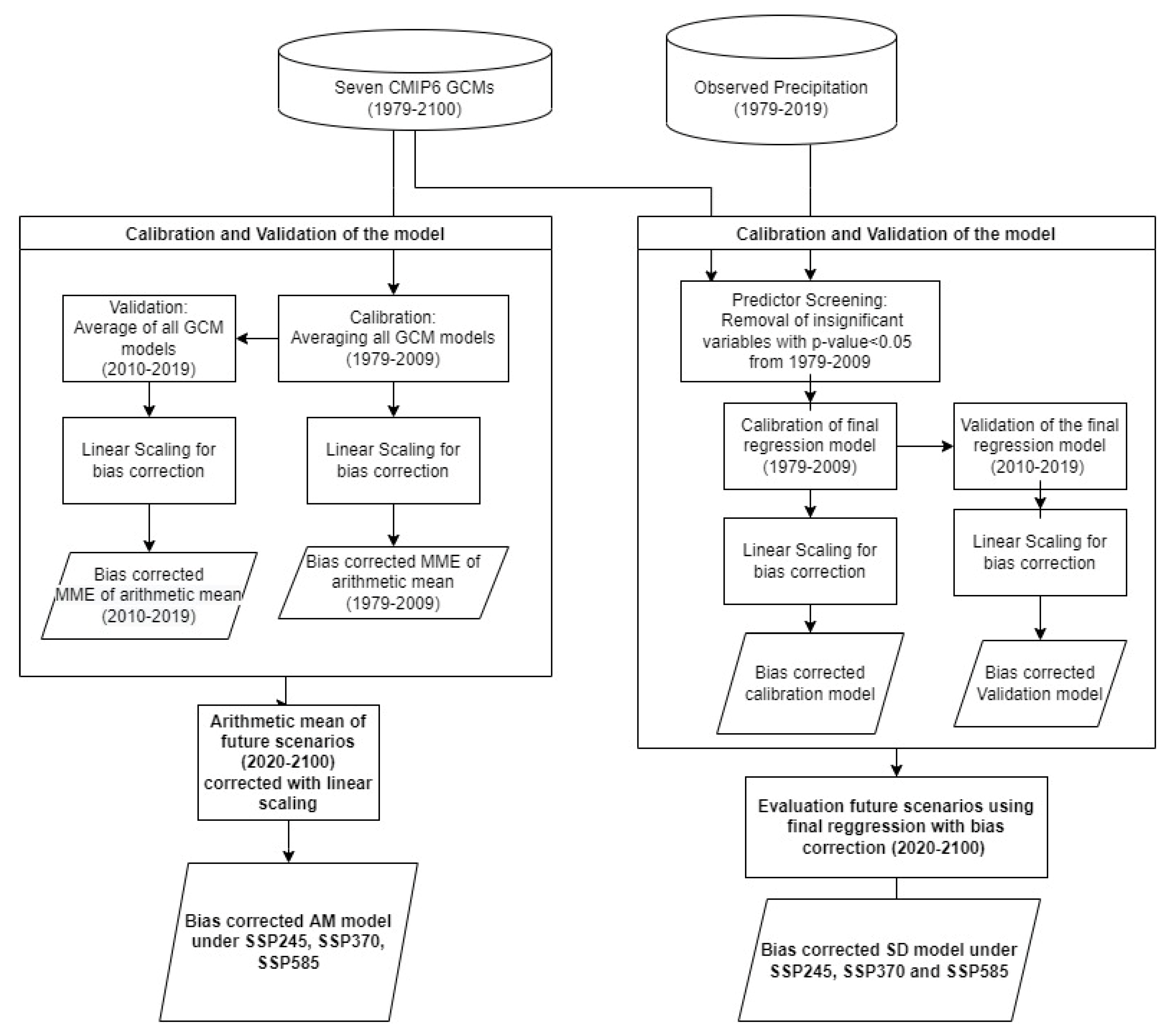
Previous similar studies in Brunei focus on several atmospheric variables in downscaling CMIP5 climate, which involves (atmospheric) predictor selections. This study tried to improve the data usage by applying a more high-resolution CMIP6, focusing on a multi-model ensemble of several CMIP6 GCM outputs, where precipitation was the sole predictor. This study thus seeks to project precipitation in Brunei Darussalam by two approaches. The first approach is to use a statistical downscaling method, MLR, with linear scaling as the bias-correcting method. The second method is to use a seven-GCM multi-model ensemble by averaging all GCMs without downscaling. Furthermore, this paper aims to assess the projected climate scenarios derived from CMIP6 models, which will be useful as input for the integration of hydrological models for the evaluation of the impacts of climate change on water resources.

2. Study Area

Brunei Darussalam is situated on the island of Borneo in Southeast Asia, covering an area of 5765 sq. km. The Belait River, Tutong River, Brunei River, and Temburong River are the major rivers that drain freshwater from the country into the sea. Most of the coastal areas are flat and swampy with alluvial depositions, whereas the inland is hilly and covered with tropical rainforests rich in biodiversity. Brunei Darussalam has a tropical equatorial climate which is hot all year round. The average annual precipitation is about 3000 mm/year, in which wet seasons with high precipitation tend to be from October to January (a total average of about 1320 mm) and May to July (a total average of about 490 mm), based on rainfall records from 1979–2019. Precipitation is not only influenced by the monsoon season but also by the Inter-Tropical Convergence Zone (ITCZ) and the localized land-sea circulation as shown in Figure 1.

3. Methodology

3.1. Data

The observed precipitation was obtained from the Brunei Darussalam Meteorological Department, in which hourly precipitation (in mm) was recorded from the station located at Brunei International Airport, at an altitude of 22 m above sea level. In this study, 41 years of observed daily precipitation (in mm) from the period 1979 to 2019 is used to validate the rainfall generated by MME of CMIP6′s precipitation from several GCM models (

Table 1. List of CMIP6 models used for MME approaches: SD and EM.

Model Name	Modeling Center	Resolution (Lon × Lat)
ACCESS-CM2	Australian Community Climate and Earth System Simulator, Australia	1.25° × 1.875°
AWI-CM-1-MR	Alfred Wegener Institute, Helmholtz Centre for Polar and Marine Research, Germany	0.94° × 0.94°
INM-CM5-0	Institute for Numerical Mathematics, Russia	2° × 1.5°
MIROC6	University of Tokyo, National Institute for Environmental Studies and Japan Agency for Marine-Earth Science and Technology, Japan	1.41° × 1.41°
MPI-ESM1-2-LR	Max Planck Institute for Meteorology, Germany	1.875° × 1.875°
MRI-ESM2-0	Meteorological Research Institute, Japan	1.125° × 1.125°
NorESM2-MM	Norwegian Climate Centre, Norway	1.25° × 0.9375°

). In previous climate downscaling studies, precipitation and temperature changes in Brunei Darussalam were generated from the predecessor GCMs from phase 5 of CMIP [17,18,27,30]. In this study, historical and future climate scenarios are obtained from https://esgf-node.llnl.gov/search/cmip6/ (accessed on 20 May 2022), which is the outcome of the coupled model intercomparison project of Phase 6 (CMIP6) under several SSP scenarios (shown in

Table 2. Summary of the selected CMIP6 scenarios for the study.

CMIP6 Scenarios	Description
SSP245	Middle-of-the-road: It considers slight improvement to economic growth with challenges to minimizing vulnerability to environmental changes persist
SSP370	Regional Rivalry: It represents the inequality in income within and between countries.
SSP585	Fossil-fueled development: It involves strong economic growth due to fossil fuel usage

) for the calibration period (1979–2009), validation period (2010–2019) and future periods (2020–2100). The future period is further broken down into three time categories: (i) near-future period (2020–2046); (ii) mid-future period (2047–2073); and (iii) far-future period (2074–2100). Each SSP scenario depends on different radiative forcing from RCPs and the projection of future rainfall by CMIP6.

The first approach is based on a statistical downscaling model using multi-linear regression, hereinafter referred to as SD, and the second approach is the arithmetic mean of a multi-model ensemble (MME). The selection of GCMs for both MME approaches is based on the availability of all scenarios of Shared Socioeconomic Pathways (SSP245, SSP270, SSP585) in the study area. These GCMs are selected based on several criteria: (i) historical runs and future scenarios for all GCMs are included in Table 1; (ii) all GCMs are available at a daily time step; and (iii) this study is a sub-model of a climate change projection that also includes maximum and minimum temperature, relative humidity, and wind speed. In which, the listed GCMs in Table 2, such climatic variables are available in the daily historical and future run.

3.2. Statistical Downscaling Model of MME (SD)

Multiple linear regression is applied to downscale precipitation based on the relationship between precipitation from seven GCMs and observed precipitation. Figure 2 is the methodology showing the steps of the downscaling process involving two stages, namely, the predictor selection and training stage, also known as the calibration stage (1979–2010) and the validation stage (2011–2019). The MLR equation initially includes all the GCM precipitation as its predictor to generate rainfall, then the predictors with a p-value greater than 0.05 are removed from the equation. This is due to p-value > 0.05 having an insignificant relationship with the predictand rainfall.

3.3. Arithmetic Mean of MME (AM)

Precipitation forecasted from the arithmetic mean (or ensemble mean) of seven GCMs is calculated by using the arithmetic mean under SSP245, SSP370, and SSP585, and the formula is as follows:

$$MME=\frac{1}{N}{{\displaystyle \sum }}_{i=1}^N{P}_i$$

(1)

Daily precipitation ($P_i)$ from nine GCMs listed in Table 1 is averaged to generate precipitation under the future SSPs. Figure 2 also represents the steps in the AM method. Similarly, the AM approach also undergoes a calibration and validation process with a bias correction using linear scaling. To evaluate the changes in precipitation throughout the future scenarios (2020–2100), three-time spans are categorized into the near future period (2020–2047), mid-future period (2048–2074) and far future period (2075–2100).

3.4. Bias Correction

A Bias correction is applied to the generated precipitation time series under the historical SSPs scenarios (1979–2019). The method used is linear scaling (LS), based on Shrestha M. [33]. LS is a simple approach to adjusting the mean of simulated precipitation to match the mean of observed precipitation in Equation (2).

$$P_{corrected}=P_{raw,m,d}\times \frac{\mu \left(P_{observed,m}\right)}{\mu \left(P_{raw,m}\right)}$$

(2)

where, $P_{corrected}$ is the corrected precipitation for all SSP scenarios and is obtained by multiplying daily precipitation simulated under SSP scenarios (denoted by $P_{raw}$) by the monthly mean observed precipitation, $P_{observed,m}$ divided by the mean monthly simulated precipitation ($P_{raw,m})$.

3.5. Performance of Model Evaluation

The next step after bias correction is to downscale SSP245, SSP370, and SSP585 generated climate parameters to obtain bias-corrected precipitation for the validation period (2011–2019) using the regression model. During the validation process, the performance of the regression model is evaluated based on a comparison between statistical indicator parameters, including mean and standard deviation, and the goodness of fit of the models, which is evaluated using the coefficient of determination (R²) and Root Mean Square Error (RMSE).

The coefficient of determination (R²) is a measure of the strength of the linear association between observed and simulated values. R² can be between zero and one, for instance, R² of 0.75 can be interpreted as 75% of the variation in observed precipitation is accounted for by the simulated precipitation values. R-squared is written as:

$$R^2=1-\frac{{{\displaystyle \sum }}_{i=1}^N{\left(y_i-\widehat{y_i}\right)}^2}{{{\displaystyle \sum }}_{i=1}^N{\left(y_i-\overline{y}\right)}^2}$$

(3)

Similar to R², RMSE is also a widely popular metric to determine how well-simulated values fit into the datasets in several studies [34,35].

$$RMSE=\frac{\sqrt{{{\displaystyle \sum }}_{i=1}^N{\left(y-\widehat{y}\right)}^2}}{\sqrt{N}}$$

(4)

The predictand (observed precipitation) and simulated precipitation are indicated as y and $\widehat{y}$, respectively, $y$ indicates the predicted value of precipitation (y), and $\overline{y}$ is the sample mean of y with sample size N.

Changes in mean precipitation for the near future (2020–2046), the mid-future (2047–2073), and the far future (2074–2100) are calculated relative to the historical period (1979–2019), by calculating the difference between the historical mean and the projected mean for their respective periods, and calculating their percentage change, as follows:

$$Changes in Precipitation=\frac{\left( mean of simulated – mean of observed\right)}{mean of observed}\times 100\%$$

(5)

4. Results and Discussion

4.1. Statistical Downscaling Model (SD)

The initial regression model of precipitation from selected GCMs as predictor variables against observed precipitation is shown in

Table 3. Initial regression model of precipitation from selected GCMs as predictor variables.

Variable	Definition	Coefficient	Std.Err.	p-Value
$a$	MRI-ESM2	−0.000230	0.017	0.989
$b$	MPI-ESM-1-2-LR	0.005601	0.029	0.846
$c$	MIROC6	−0.020	0.019	0.314
$d$	NOR-ESM2-MM	0.036	0.018	0.046
$e$	INM-CSM-0	0.036	0.016	0.024
$f$	ACCESS_CM2	0.050	0.021	0.019
$g$	AWI-CM-1-MR	0.047	0.017	0.006
	Constant	6.705	0.439	0.000

, y before the reduction in variables is written as

$$y=-0.000230 a+0.005601 b-0.020 c+0.036 d+0.036 e+0.050 f+0.047 g+6.705$$

(6)

Three insignificant variables from (MRI-ESM2, MPI-ESM-1-2-LR and MIROC6) are removed due to p-value greater and equal to 0.05, whereas, the predictors listed below ($x_1$–$x_4$) exhibits p-value < 0.05, showing that there is a statistically significant relationship between the observed and the predictors. Hence, the final regression model is written as in Equation (7), which generates the precipitation time series for the SD model under all SSP scenarios as shown in

Table 4. Final regression model with satistical parameters.

Variable	Definition	Coefficient	Std.Err.	p-Value
	Constant	6.601	0.363	0.000
$x_1$	ACCESS-CM2	0.049	0.021	0.020
$x_2$	AWI-CM-1-MR	0.046	0.017	0.006
$x_3$	INM_-SM_-	0.036	0.016	0.026
$x_4$	NOR-ESM2-MM	0.035	0.018	0.053

.

$$y=0.049 x_1+0.046 x_2+0.036 x_3+0.035 x_4+6.601$$

(7)

4.2. Calibration and Validation of the Models

Validation of the model is measured based on the daily mean, root mean square error (RMSE), and determination of coefficient (R²) of average monthly for observed data, ensemble mean of seven GCM data, and statistical downscaling precipitation (SD) after bias adjustment.

Table 5. Summary of mean and standard deviation for calibration and validation period before and after bias correction for SD model and AM model.

		Before Bias Correction			After Bias Correction
Calibration (1979–2009)	Time Series	Mean	NSE	R2	Mean	NSE	R2
	Obs	8.13
	SD	13.90	−0.63	0.82	8.13	1.00	1.00
	EM	8.48	0.48	0.71	8.13	1.00	1.00
Validation (2010–2019)	Obs	8.97
	SD_SSP245	11.90	115.04	0.33	7.08	75.74	0.85
	SD_SSP370	12.16	119.826	0.42	6.92	71.02	0.86
	SD_SSP585	12.07	118.15	0.39	7.84	89.812	0.84
	EM_SSP245	8.13	85.22	0.22	7.74	57.37	0.83
	EM_SSP370	8.13	85.22	0.22	7.64	61.15	0.80
	EM_SSP585	7.05	73.07	0.23	7.48	66.60	0.77

summarizes the comparison of these statistical measurements for monthly average observed and corrected data under calibration and validation periods before and after bias adjustment. Before bias adjustment, the AM model has the closest mean value of (µ = 8.48) in the calibration period. The mean for bias-corrected SD precipitation (under all SSP scenarios) improved significantly (Supplementary Materials), ranging from 6.29 to 7.84, matching the mean of observed precipitation (µ = 8.97). After bias correction of AM for the validation period, there are mean differences ranging from 7.48 to 7.74 between the mean of the observed data (µ = 8.97) and bias-corrected SSP scenarios. Table 5 also compares the R² and RMSE values for the AM and SD models of the SSP245, SSP370, and SSP585 scenarios. The results showed that there was an improvement achieved in bias-corrected precipitation simulated by the SD model. The highest correlation with observed precipitation is found for SSP370 (R² = 0.86), while SSP245 and SSP585 show also a very good correlation with the observed time-series (minimum R² = 0.85 and 0.84). After bias correction, the RMSE of SD precipitation improves significantly more than AM. Moreover, the bias-corrected AM model resulted in a lower R² than the SD model and RMSE values. The result indicates that corrected SD under the SSP245 scenario yields better performance in terms of RMSE and R² values. Therefore, the statistical metric in Table 5 shows that the SD model outperforms the arithmetic mean (AM) for the validation period after bias correction (2015–2019). Figure 3 shows the boxplot displaying the observed and the simulated precipitation to show the variability of the data. For the annual precipitation, both models seem to diverge significantly from the observed data, but the similarity in median precipitation with the observed data. In terms of monthly variations, the two models were able to capture the same variance and median with the reference data. These findings suggest that the bias correction with linear scaling may be suitable for improving the mean of the monthly variation following the observed data, in comparison to annual precipitation. Further investigation is required to compare the performance of the model in terms of annual precipitation with different bias correction methods, such as power transformation or variance scaling.

Figure 4 shows the downscaled MME by statistical downscaling (SD) and arithmetic mean (AM) results for the validation period compared to the baseline period. After bias correction, average monthly SD and AM precipitation generates the typical highest rainfall amount of the baseline period during January, November, and December, compared to the rest of the month. However, they still tend to show significant underestimation for the months of January, November, and December in comparison to observed precipitation.

Although the SSP370 time series for corrected SD precipitation follows the observed trend closer than others, the biggest overestimation can be found in October under SSP245 and SSP370. On the other hand, AM shows significant improvement after bias correction, but it has a slight overestimation of the average monthly rainfall in August (under SSP370 and SSP585), October (under SSP245and SSP370), and March (under SSP585). Throughout the validation period, SD models under all SSP scenarios give the best outcome, as the SD time series follows the closest trend to the observed precipitation.

4.3. Future Projection of Precipitation

The future projection of precipitation is divided into three time slices: the near future period (2020–2046), the mid-future period (2047–2073), and the far future (2047–2100). Overall, the trend of precipitation in the late 21st century for SSP scenarios generated by SD and AM precipitation follows the observed trend but with some underestimation and overestimation for some scenarios and months. Figure 5a–c represents the comparison of monthly variation between the arithmetic mean (AM) and the downscaled future MME (SD) under different SSP scenarios after bias correction. SD generated future precipitation with lower monthly precipitation compared to AM precipitation. Towards the end of the century, the rainy season from October-December under the SD approach will experience a slight increase in monthly precipitation compared to the previous mid-future period. On the other hand, the future precipitation by the AM model has smaller differences with the observed rainfall shown in Figure 5. However, AM also produced a similar lower rainfall amount than the previous SD Near and Mid-future time series during the wet season (October, November, and December). Furthermore, the far-future period under the AM approach forecasted the same average rainfall amount as the baseline period. Similarly, months with a lesser precipitation amount (February and April) remain the same for both SD and AM models throughout the future periods. From an agricultural perspective, a lower precipitation trend in the future, especially during the wet season, may affect the agricultural water needs for rain-fed crops, leading to crop failure. More irrigation may be required, and precautionary actions should be taken to adapt to the changing climate. Such adaptations are deficit irrigation scheduling methods to estimate the proper amount and timing during those lower rainy occurrences; farmers should start to rely on a water-saving irrigation method such as alternate wetting and drying water regime [36].

Annual precipitation for future scenarios under SD and AM approaches can be observed in Figure 6. It is predicted that the precipitation time series generated under the SD model will have a steady increase and the lowest annual precipitation trend. The EM model simulated a higher amount of annual precipitation than the SD model. These findings also coincide with the previous work by Hasan et al. (2018), in which a downward trend is detected in the future precipitation based on CMIP5 future scenarios under HadCM3 A1B and CGCM3 A1B, but a more fluctuating trend is observed for annual precipitation under CanESM2 [15].

Table 6. Changes in future precipitation in comparison to observed mean of 3041.2 mm.

	Precipitation Change (%)
	Near Future	Mid Future	Far Future
	(2020–2046)	(2047–2073)	(2074–2100)
SD_SSP245	−27.3	−27.1	−17.7
SD_SSP370	−27.8	−27.8	−18.5
SD_SSP585	−27.6	−25.4	−16.7
AM_SSP245	−10.8	−11.1	−14.4
AM_SSP370	−11.7	−9.4	−17.6
AM_SSP585	−12.1	−8.4	−18.7

presents the changes in annual precipitation in the three future periods. Under the SD approach, the annual precipitation is reduced significantly by approximately 28% in the near and mid future for all SSP scenarios. Towards the end of the century, the SD projected an increasing trend as the precipitation change began to reduce by at least 16.7% (SSP585). On the contrary, the AM model predicted a smaller precipitation change but with a steady decreasing trend towards the far future. This result is in contrast with the study reported by Dk Fathiyah et al. (2021), where the annual CMIP5 precipitation projection in Brunei was predicted to have a more chaotic nature with a significant increasing trend. Hasan et al. (2018), and Dk Fathiyah et al., (2021) applied SDSM and statistical downscaling with backward regression, respectively, and yielded different outcomes for the same region in comparison to this study. This may be due to the use of several atmospheric predictors to develop the SD model.

5. Conclusions

A Multi-Model Ensemble (MME) of CMIP6 precipitation is applied to forecast future rainfall in Brunei Darussalam. The predictor variables of seven CMIP6 GCM precipitation from 1979 to 2009 are used to develop the relationship with observed daily and monthly precipitation obtained from BMDB. The first approach is statistical downscaling by evaluating the relationship between observed rainfall and the selected CMIP6 GCM predictors using multiple linear regression. The second MME approach is the arithmetic mean of seven CMIP6 GCMs by taking all the mean of seven precipitations with bias correction of linear scaling. During the validation period, linear scaling has significantly improved monthly precipitation with both SD and AM models, and there is a reasonable agreement with observation. However, linear scaling shows poor performance in the annual precipitation for both SD and AM.

The precipitation projection based on the arithmetic mean suggests an Increasing trend in the future with both monthly and annual precipitation consistently below the observation. Statistical downscaling of MME predicted a steady decreasing trend during the near and mid-future periods, but with a slight increase in the far future term. This study provides a climate scenario as input for simulating hydrological models to help assess future water resources and/or monitor potential drought spells. Further research needed to be carried out includes incorporating other bias corrections such as Power transformation or Quantile Mapping to produce a better performance of annual precipitation, and spatial change of precipitation based on available satellite data can also be useful. Furthermore, the arithmetic mean model can be improved further through careful selection of GCM models by ranking their performance based on statistical metrics, empirical cumulative distribution function (ECDF), and Taylor skillscore (TSS) [37].

References

1. Hoang, L.P.; Lauri, H.; Kummu, M.; Koponen, J.; Van Vliet, M.T.; Supit, I.; Leemans, R.; Kabat, P.; Ludwig, F. Mekong River flow and hydrological extremes under climate change. Hydrol. Earth Syst. Sci. 2016, 20, 3027–3041. [Google Scholar] [CrossRef]
2. Uk, S.; Yoshimura, C.; Siev, S.; Try, S.; Yang, H.; Oeurng, C.; Li, S.; Hul, S. Tonle Sap Lake: Current status and important research directions for environmental management. Lakes Reserv. Res. Manag. 2018, 23, 177–189. [Google Scholar] [CrossRef]
3. Energy and Industry Department. Brunei Darussalam’s Second National Communication: Under the United Nations Framework Convention on Climate Change; The Prime Minister’s Office: Singapore, 2017.
4. Yuan, C.; Yamagata, T. Impacts of IOD, ENSO and ENSO Modoki on the Australian Winter Wheat Yields in Recent Decades. Sci. Rep. 2015, 5, 17252. [Google Scholar] [CrossRef]
5. Guven, A.; Aytek, A. New Approach for Stage–Discharge Relationship: Gene-Expression Programming. J. Hydrol. Eng. 2009, 14, 812–820. [Google Scholar] [CrossRef]
6. Adib, M.N.M.; Harun, S.; Rowshon, M.K. Long-term rainfall projection based on CMIP6 scenarios for Kurau River Basin of rice-growing irrigation scheme, Malaysia. SN Appl. Sci. 2022, 4, 70. [Google Scholar] [CrossRef]
7. Ayugi, B.; Shilenje, Z.W.; Babaousmail, H.; Lim Kam Sian, K.T.C.; Mumo, R.; Dike, V.N.; Iyakaremye, V.; Chehbouni, A.; Ongoma, V. Projected changes in meteorological drought over East Africa inferred from bias-adjusted CMIP6 models. Nat. Hazards 2022, 1–26. [Google Scholar] [CrossRef] [PubMed]
8. Hamed, M.M.; Nashwan, M.S.; Shahid, S.; Ismail, T.B.; Dewan, A.; Asaduzzaman, M. Thermal bioclimatic indicators over Southeast Asia: Present status and future projection using CMIP6. Environ. Sci. Pollut. Res. 2022, 1–20. [Google Scholar] [CrossRef] [PubMed]
9. Riahi, K.; van Vuuren, D.P.; Kriegler, E.; Edmonds, J.; O’Neill, B.C.; Fujimori, S.; Bauer, N.; Calvin, K.; Dellink, R.; Fricko, O.; et al. The Shared Socioeconomic Pathways and their energy, land use, and greenhouse gas emissions implications: An overview. Glob. Environ. Chang. 2017, 42, 153–168. [Google Scholar] [CrossRef]
10. Mahmood, R.; Babel, M.S. Future changes in extreme temperature events using the statistical downscaling model (SDSM) in the trans-boundary region of the Jhelum river basin. Weather Clim. Extrem. 2014, 5–6, 56–66. [Google Scholar] [CrossRef]
11. Hossain, I.; Rasel, H.; Imteaz, M.A.; Mekanik, F. Long-term seasonal rainfall forecasting: Efficiency of linear modelling technique. Environ. Earth Sci. 2018, 77, 280. [Google Scholar] [CrossRef]
12. Islam, F.; Imteaz, M.A. Development of prediction model for forecasting rainfall in Western Australia using lagged climate indices. Int. J. Water 2019, 13, 248–268. [Google Scholar] [CrossRef]
13. Hussain, M.; Yusof, K.W.; Mustafa, M.R.; Afshar, N.R. Application of statistical downscaling model (SDSM) for long term prediction of rainfall in Sarawak, Malaysia. In Water Resources Management VII; WIT Press: Southampton, UK, 2015; Volume 196, pp. 269–278. [Google Scholar]
14. Aziz, K.S.A.; Shams, S.; Rahman, E.K.A.; Ratnayake, U. An Analysis of Statistical Correlation for Downscaled Precipitation Data. In Proceedings of the 7th Brunei International Conference on Engineering and Technology 2018 (BICET 2018), Univerisiti Teknologi Brunei, Bandar Seri Begawan, Brunei, 12–14 November 2018. [Google Scholar]
15. Hasan, D.S.N.A.b.P.A.; Ratnayake, U.; Shams, S.; Nayan, Z.B.H.; Rahman, E.K.A. Prediction of climate change in Brunei Darussalam using statistical downscaling model. Theor. Appl. Climatol. 2018, 133, 343–360. [Google Scholar] [CrossRef]
16. Dk Fathiyah, P.S.; Ratnayake, U.; Rashid, A.A.; Rahman, E.K.A. The Comparison of Bias Correction Methods in Statistical Downscaling Precipitation in Brunei Darussalam. In Proceedings of the The 8th Brunei International Conference on Engineering and Technology, Bandar Seri Begawan, Brunei, 8–10 November 2021. [Google Scholar]
17. Shashikanth, K.; Sukumar, P. Indian Monsoon Rainfall Projections for Future Using GCM Model Outputs Under Climate Change. Res. India Publ. 2017, 10, 1501–1516. [Google Scholar]
18. Try, S.; Tanaka, S.; Tanaka, K.; Sayama, T.; Khujanazarov, T.; Oeurng, C. Comparison of CMIP5 and CMIP6 GCM performance for flood projections in the Mekong River Basin. J. Hydrol. Reg. Stud. 2022, 40, 101035. [Google Scholar] [CrossRef]
19. Su, X.; Shao, W.; Liu, J.; Jiang, Y. Multi-Site Statistical Downscaling Method Using GCM-Based Monthly Data for Daily Precipitation Generation. Water 2020, 12, 904. [Google Scholar] [CrossRef]
20. Liang, J.; Tan, M.L.; Hawcroft, M.; Catto, J.L.; Hodges, K.I.; Haywood, J.M. Monsoonal precipitation over Peninsular Malaysia in the CMIP6 HighResMIP experiments: The role of model resolution. Clim. Dyn. 2022, 58, 2783–2805. [Google Scholar] [CrossRef]
21. Tan, B.T.; Fam, P.S.; Firdaus, R.B.R.; Tan, M.L.; Gunaratne, M.S. Impact of Climate Change on Rice Yield in Malaysia: A Panel Data Analysis. Agriculture 2021, 11, 569. [Google Scholar] [CrossRef]
22. Juneng, L.; Tangang, F.T.; Kang, H.; Lee, W.-J.; Seng, Y.K. Statistical Downscaling Forecasts for Winter Monsoon Precipitation in Malaysia Using Multimodel Output Variables. J. Clim. 2010, 23, 17–27. [Google Scholar] [CrossRef]
23. Wang, D.; Liu, J.; Shao, W.; Mei, C.; Su, X.; Wang, H. Comparison of CMIP5 and CMIP6 Multi-Model Ensemble for Precipitation Downscaling Results and Observational Data: The Case of Hanjiang River Basin. Atmosphere 2021, 12, 867. [Google Scholar] [CrossRef]
24. Wang, B.; Jin, C.; Liu, J. Understanding Future Change of Global Monsoons Projected by CMIP6 Models. J. Clim. 2020, 33, 6471–6489. [Google Scholar] [CrossRef]
25. Supharatid, S.; Nafung, J.; Aribarg, T. Projected changes in temperature and precipitation over mainland Southeast Asia by CMIP6 models. J. Water Clim. Chang. 2022, 13, 337–356. [Google Scholar] [CrossRef]
26. Masud, B.; Cui, Q.; Ammar, M.E.; Bonsal, B.R.; Islam, Z.; Faramarzi, M. Means and Extremes: Evaluation of a CMIP6 Multi-Model Ensemble in Reproducing Historical Climate Characteristics across Alberta, Canada. Water 2021, 13, 737. [Google Scholar] [CrossRef]
27. Ngoma, H.; Wen, W.; Ayugi, B.; Babaousmail, H.; Karim, R.; Ongoma, V. Evaluation of precipitation simulations in CMIP6 models over Uganda. Int. J. Climatol. 2021, 41, 4743–4768. [Google Scholar] [CrossRef]
28. Mishra, V.; Bhatia, U.; Tiwari, A.D. Bias-corrected climate projections for South Asia from Coupled Model Intercomparison Project-6. Sci. Data 2020, 7, 338. [Google Scholar] [CrossRef] [PubMed]
29. Yan, Y.; Zhu, C.; Liu, B.; Jiang, S. Annual Cycle of East Asian Precipitation Simulated by CMIP6 Models. Atmosphere 2020, 12, 24. [Google Scholar] [CrossRef]
30. Guo, H.; Bao, A.; Chen, T.; Zheng, G.; Wang, Y.; Jiang, L.; De Maeyer, P. Assessment of CMIP6 in simulating precipitation over arid Central Asia. Atmos. Res. 2021, 252, 105451. [Google Scholar] [CrossRef]
31. Kang, S.; Hur, J.; Ahn, J. Statistical downscaling methods based on APCC multi-model ensemble for seasonal prediction over South Korea. Int. J. Climatol. 2014, 34, 3801–3810. [Google Scholar] [CrossRef]
32. Hasan, D.S.N.A.B.P.A.; Ratnayake, U.; Shams, S. Evaluation of rainfall and temperature trends in Brunei Darussalam. AIP Conf. Proc. 2016, 1705, 020034. [Google Scholar]
33. Shrestha, M. Data analysis relied on Linear Scaling bias correction (V.1.0) Microsoft Excel file. 2015. [Google Scholar]
34. Akhter, J.; Das, L.; Meher, J.K.; Deb, A. Evaluation of different large-scale predictor-based statistical downscaling models in simulating zone-wise monsoon precipitation over India. Int. J. Climatol. 2019, 39, 465–482. [Google Scholar] [CrossRef]
35. Molina, O.D.; Bernhofer, C. Projected climate changes in four different regions in Colombia. Environ Syst Res. 2019, 8, 33. [Google Scholar] [CrossRef]
36. Yang, C.-M. Technologies to Improve Water Management for Rice Cultivation to Cope with Climate Change. Crop. Environ. Bioinform. 2012, 8, 193–207. [Google Scholar]
37. Babaousmail, H.; Hou, R.; Ayugi, B.; Ojara, M.; Ngoma, H.; Karim, R.; Rajasekar, A.; Ongoma, V. Evaluation of the Performance of CMIP6 Models in Reproducing Rainfall Patterns over North Africa. Atmosphere 2021, 12, 475. [Google Scholar] [CrossRef]
Figure 1. Map of rainfall trend in the study area [32].
Hydrology 09 00161 g001
Figure 2. Schematic flowchart of the methodology.
Hydrology 09 00161 g002
Figure 3. Box plot of annual and monthly simulated precipitation by SD and AM model, N = 30 years.
Hydrology 09 00161 g003
Figure 4. Validation Period (2015–2019) under for SD and AM approach under the figure.
Hydrology 09 00161 g004
Figure 5. Comparison of monthly average precipitation based on SD and AM model for the figure.
Hydrology 09 00161 g005aHydrology 09 00161 g005b
Figure 6. Annual Precipitation generated by SD and AM model relative to the observed precipitation.
Hydrology 09 00161 g006