Article

Suitability Assessment of Fish Habitat in a Data-Scarce River

1
Department of Civil Engineering, Chittagong University of Engineering & Technology (CUET), Chittagong 4349, Bangladesh
2
Associate Environmental Engineer, Streams Tech Limited, Dhaka 1213, Bangladesh
3
Assistant Town Planner, Chattogram Development Authority (CDA), Chittagong 4349, Bangladesh
*
Author to whom correspondence should be addressed.
Hydrology 2022, 9(10), 173; https://doi.org/10.3390/hydrology9100173
Submission received: 30 July 2022 / Revised: 20 September 2022 / Accepted: 27 September 2022 / Published: 3 October 2022
(This article belongs to the Special Issue Stochastic and Deterministic Modelling of Hydrologic Variables)

Abstract

:
Assessing fish habitat suitability in a data-scarce tidal river is often challenging due to the absence of continuous water quantity and quality records. This study is comprised of an intensive field study on a 42 km reach which recorded bathymetry and physical water quality parameters (pH, electroconductivity, dissolved oxygen, and total dissolved solids) testing and corresponding water levels and velocity. Frequent water sampling was carried out on 17 out of 90 locations for laboratory water quality tests. Based on this, an interpolation technique, i.e., Inverse Distance Weighted (IDW), generates a map in a Geographic Information System (GIS) environment using ArcGIS software to determine the river water quality parameters. Additionally, a hydrodynamic model study was conducted to simulate hydraulic parameters using Delft3D software followed by a water quality distribution. During validation, the Delft3D-simulated water quality could reasonably mimic most field data, and GIS featured dissolved oxygen. The overall water quality distribution showed a lower dissolved oxygen level (~3 mg/L) in the industrial zone compared to the other two zones during the study period. On the other hand, these validated hydraulic properties were applied in the Physical Habitat Simulation Model (PHABSIM) set up to conduct the hydraulic habitat suitability for Labeo rohita (Rohu fish). Thus, the validated model could represent the details of habitat suitability in the studied river for future decision support systems, and this study envisaged applying it to other similar rivers.

1. Introduction

Increased urbanization and industrialization threaten the adjacent river’s water quantity and quality. Dissolved oxygen (DO), chemical oxygen demand (COD), and biochemical oxygen demand (BOD) are the essential parameters for assessing river water quality. Drastic reduction in DO in the waterbody causes the suffocation and loss of aquatic plants and animals, leading to the deterioration of overall water quality and causes a threat to the river’s ecological balance [1,2]. Thus, an appropriate monitoring network is essential to obtain a comprehensive view of water quality [3] and generally, installing a network is expensive. Spatial and temporal analysis of river water quality often provides valuable information on a particular water quality parameters. In this regard, the Geographic Information System (GIS), which is a practical spatial tool widely used to predict, monitor, and manage, might offer geographic information visualization. Additionally, a numerical model could be an excellent basis for featuring present and future insights. The river water quality model generally consists of the hydrodynamic and dispersion models. In recent years, numerous hydrodynamic and water quality models have been developed. Some recent studies have assessed the discharge requirements of spawning fish empirically at the reach scale [4,5,6], the interaction of channel morphology and discharge influences the distribution of spawning [7,8,9], and physical habitat changes associated with river flow [5,10,11,12,13].Data consistency and regularity are essential parts of a smooth simulation. On the other hand, predictive models based on field observation data can dispute that investigation. From a mathematical perspective, in most cases, the differential equation has been solved with the finite difference technique to obtain a practical model scenario [14,15,16]. It is able to deal with the original 1D steady-state model up to 3D model for the transient and unsteady flow simulation [17]. Among the available numerical models, Delft3D has incorporated the advanced concepts considering both hydrodynamic flow and water quality (D-WAQ) perspectives for the river, lake, or shore [18,19]. The Physical Habitat Simulation (PHABSIM) model is a set of numerical models engaged in assessing the physical habitat of a water body in terms of the amalgamation of discharge, velocity, and particular depth [10,12,20,21,22,23,24,25,26]. This model is mostly applied to assess the availability of suitable habitats for fish, macrophytes [27,28,29], and macroinvertebrates [30]. Thus, PHABSIM can be applied to assess habitat suitability over a range of river flows to predict variations in flow regimes due to river morphology changes and can be incorporated into river rehabilitation schemes.
The Karnafuli River flows over the industrial capital of Bangladesh, i.e., Chittagong, and accommodates around 800 industries on or adjacent to the riverbank of Karnafuli [31]. Increasing trends were recorded in the industrial growth on this river, adding river pollution by disposing untreated wastewater [32]. Similarly, as urbanization progressed, the urban population was 4.3% in Chittagong in 1950, which increased to 30.8% in 2015 [33]. A recent study identified higher trace elements (i.e., arsenic, chromium, cadmium, and lead) among different fish species in this river [4]. So far, considering the river water quantity and quality, there is possibly no study on the habitat suitability establishment except for a few water quality studies, i.e., salinity [34]. This reported study started with an intensive field survey and then spatial and temporal analysis to validate a hydrodynamic model. An interpolation technique, i.e., Inverse Distance Weighted (IDW), generates a map using ArcGIS software to determine DO’s spatial and temporal analysis in the river. Labeo rohita is the native fish in the Kshipra River at Dewas in India, and this river maintains the Indian standards; the permissible DO is of 6–8 mg/L [35]. Labeo rohita (Rohu fish) of the carp family is typically a cyprinid shape and is available in the rivers of South Asia. Thus, the Delft3D model could be applied to simulate the flow and representative water quality parameters of the Karnafuli River to establish a relationship between river flow and water quality. Finally, this study involved PHABSIM to demonstrate the physical habitat area for Labeo rohita that exists upstream of the Karnafuli River.

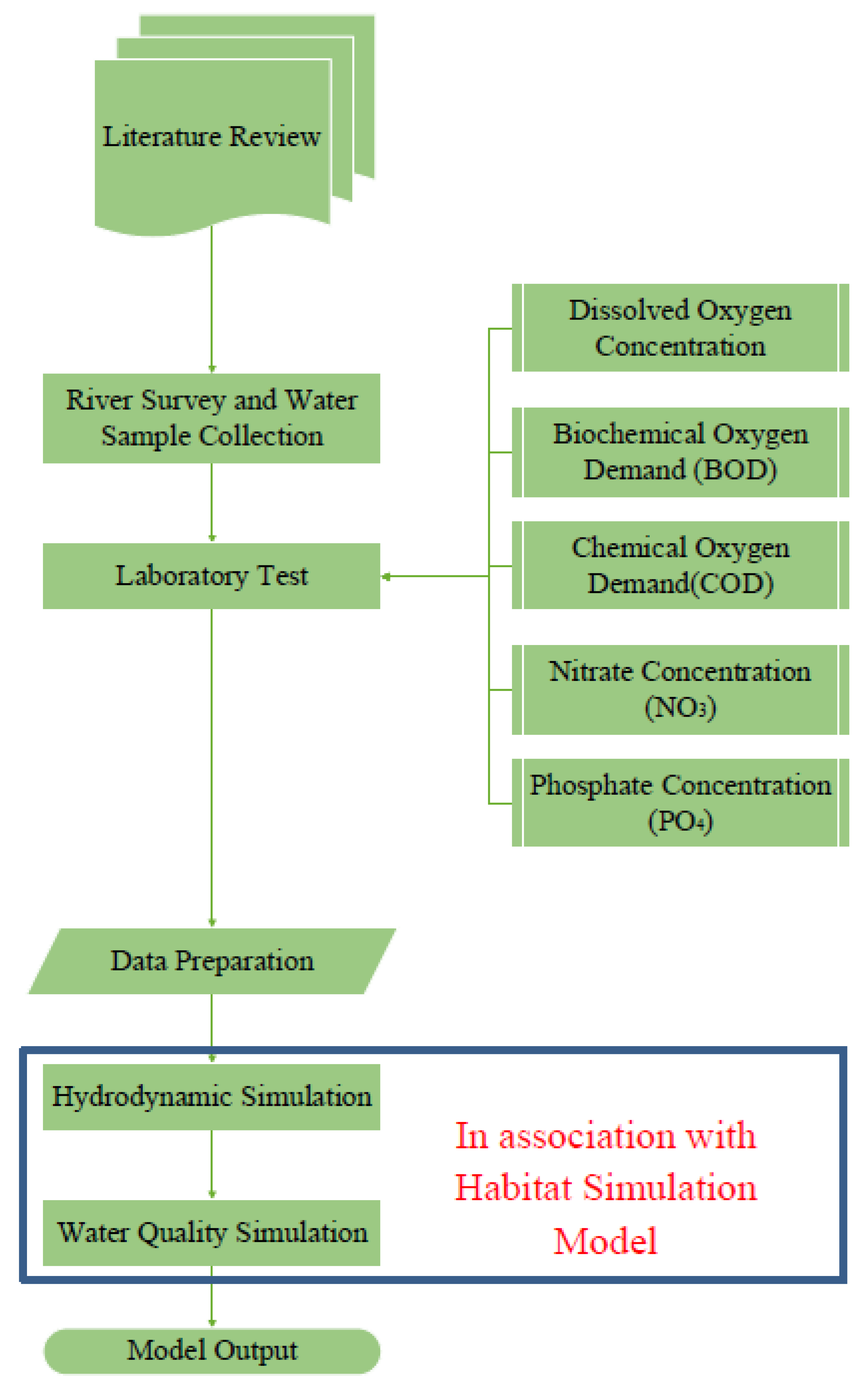
2. Materials and Methodology
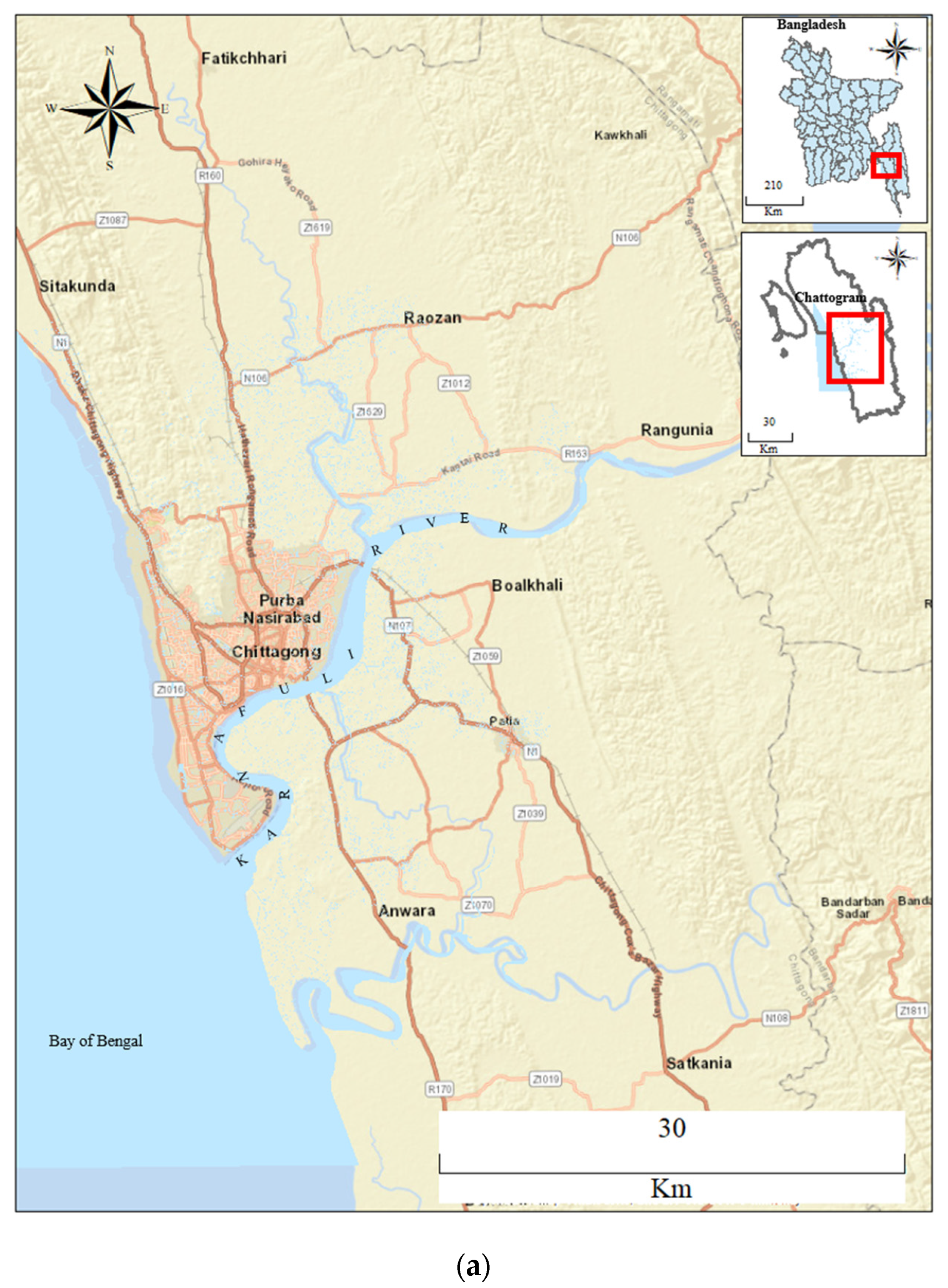
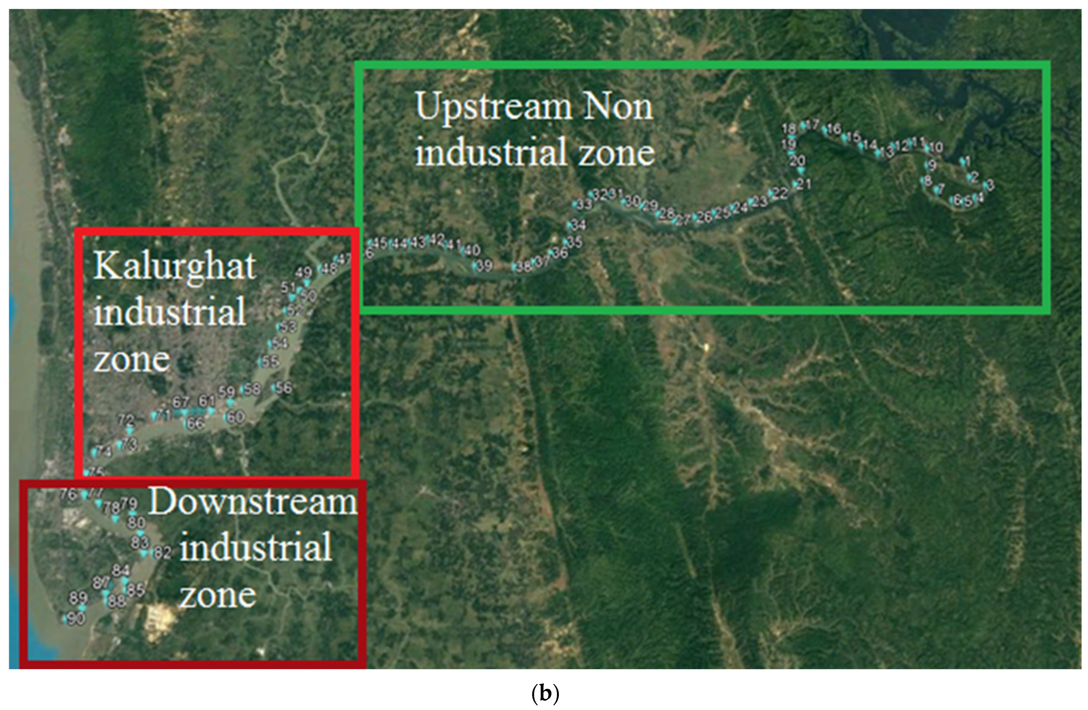
In this study, the numerical model setup requires primary and secondary datasets. From October 2019 to January 2021, the primary dataset was comprised of a river bathymetry survey, water sampling, and laboratory tests. Secondary data were collected for water level and flow data acquisition. Sampling was conducted considering the importance of DO, COD, BOD, nitrate, and phosphate on the river ecosystem as well as the fish habitat. As the hourly measurement of DO using a portable DO meter has been done longitudinally while sampling from upstream to downstream, laboratory tests were required for better understanding. According to the American Public Health Association (APHA), American Water Works Association (AWWA), and Water Environment Federation (WEF), APHA Method 4500-NO3 and 4500-P Phosphorus were applied for nitrate and phosphate tests.
In a GIS environment, different interpolation methods are usually practiced for surface interpolation. Among them, three interpolation modes are widely used: Inverse Distance Weighted (IDW), Spline, and Kriging. The IDW method was used due to flexibility in data estimation. A hydrodynamic model study was carried out using Delft3D and, after validation, was applied to the water quality simulation. Finally, the water quality model was validated using the available field data (Figure 1). Then, PHABSIM allowed the prediction of usable physical habitat areas for river species at different life stages. The functional physical habitat area is usually demonstrated as Weighted Usable Area (WUA) in sq m per 1000 m river channel. WUA was measured by combining physical habitat quantity and quality for the specific discharge and species/life stage.

2.1. Study Area

The Karnafuli River (between 22°12′60.00″ N and 91°47′59.99″ E), which originated from the Lushai hills in the Mizoram state of India, is one of the most important and largest rivers for the Chittagong city and the Chittagong hill tracts. With a total length of 180 km, the steep waterway passes Rangamati at a confined loop and progresses as a zigzag course toward two more main loops in the Dhuliachhari and the Kaptai. Starting from the Kaptai loop, the river meandering covers the Sitapahar hill range and, thus, flows across the plain of Chittagong through Chandraghona hills and drains into the Bay of Bengal. Upstream river Halda, which falls into the Karnafuli river, is Bangladesh’s only pure Indian carp breeding field, perhaps the only one in South Asia. Thus, Karnafuli might also play an important role in ‘Carp’ fish habitats. The selected site is 42 km away from the upstream of the Karnafuli to the downstream towards the estuary. Three different depth-wise (i.e., bottom, mid-depth, upper surface) water samples were collected for each sampling point throughout the river at every 1 km interval (Figure 2a,b). During sampling, onsite hourly DO measurements were carried out. For the intensive laboratory tests during 2020–2021, 17 water sampling points among the 90 water sampling points were selected, and these were: three (#10, #22, and #32) in the upstream non-industrial zone; seven points in the Kalurgaht industrial zone (#48, #49, #51, #54, #59, #60, and #61), and seven points in downstream industrial zone (#62, #67, #70, #71, #74, #76, and #89), respectively (Figure 2b).

2.2. Primary Dataset

The primary dataset is comprised of river surveys and water samplings for field and laboratory tests. A river bathymetry survey was conducted using a map plotter of the Garmin GPS; thus, its ultrasound measured the pointwise water depth. These records were validated against the collected bathymetric data from the Chittagong Port Authority (CPA), then used in the model setup. DO was measured hourly using portable equipment (Lutron DO-5509 Portable DO Meter, Taiwan) according to the Standard Methods for the Examination of Water and Wastewaters [36] at the surface, middle, and near-bottom (1 m over the riverbed), as stated in Section 2.1. The laboratory test dataset validated field-tested DO values for each of the 90 sampling sites (Figure 2b). Then, a field test was carried out for pH, electroconductivity, DO, and TDS.
The collected samples were tested in a laboratory for dissolved oxygen, BOD5, and COD. Nitrate and phosphate were tested using Nitraver 5 Nitrate Reagent and PhosVer® 3 Phosphate Reagent, Hach Company, USA, respectively. For this study, the CODcr method was used to determine COD [16]. After five days of incubation, BOD5 was recorded following Bajpai 2018 [37]. BOD5 could be represented by CBOD or carbonaceous biochemical oxygen demand [38]. The CBOD indicates the depletion of dissolved oxygen from both carbonaceous and nitrogenous actors in a contaminated water sample.

2.3. Secondary Dataset

The bathymetry data of the river were obtained from the Chittagong Port Authority (CPA) and the Bangladesh Water Development Board (BWDB). The hydrodynamic data (water level and discharge) were incorporated in this study. The upstream releases from Kaptai were collected as a time series and then used as the upstream boundary condition for the model.

3. Model Study

The water quality module depends on the hydrodynamic simulation. The eight water quality parameters discussed were included as the substance in the model. The model’s time frame and time step were similar to the hydrodynamic simulation. The time series variation in the concentration of different substances was the boundary condition for upstream and downstream boundaries.

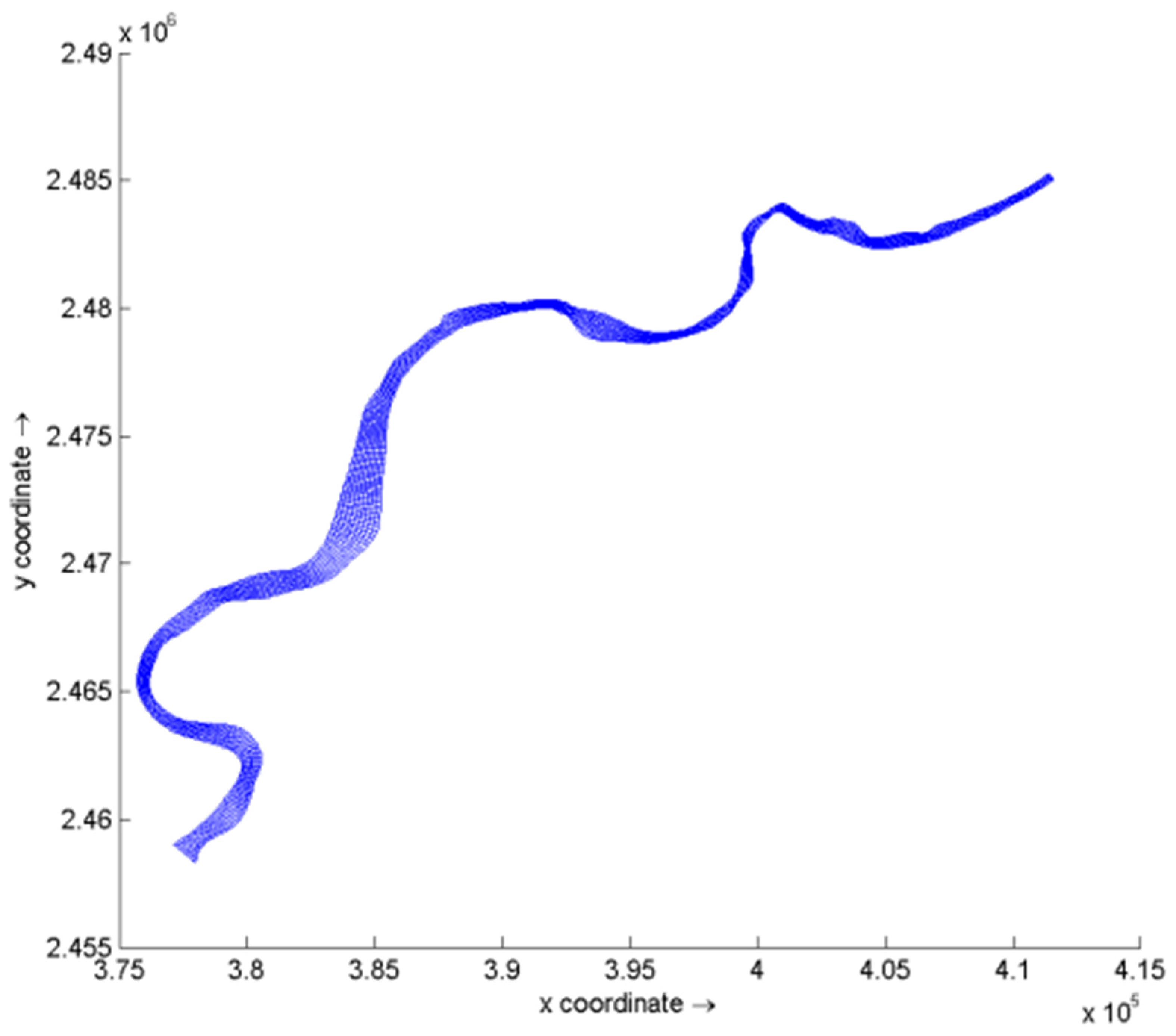
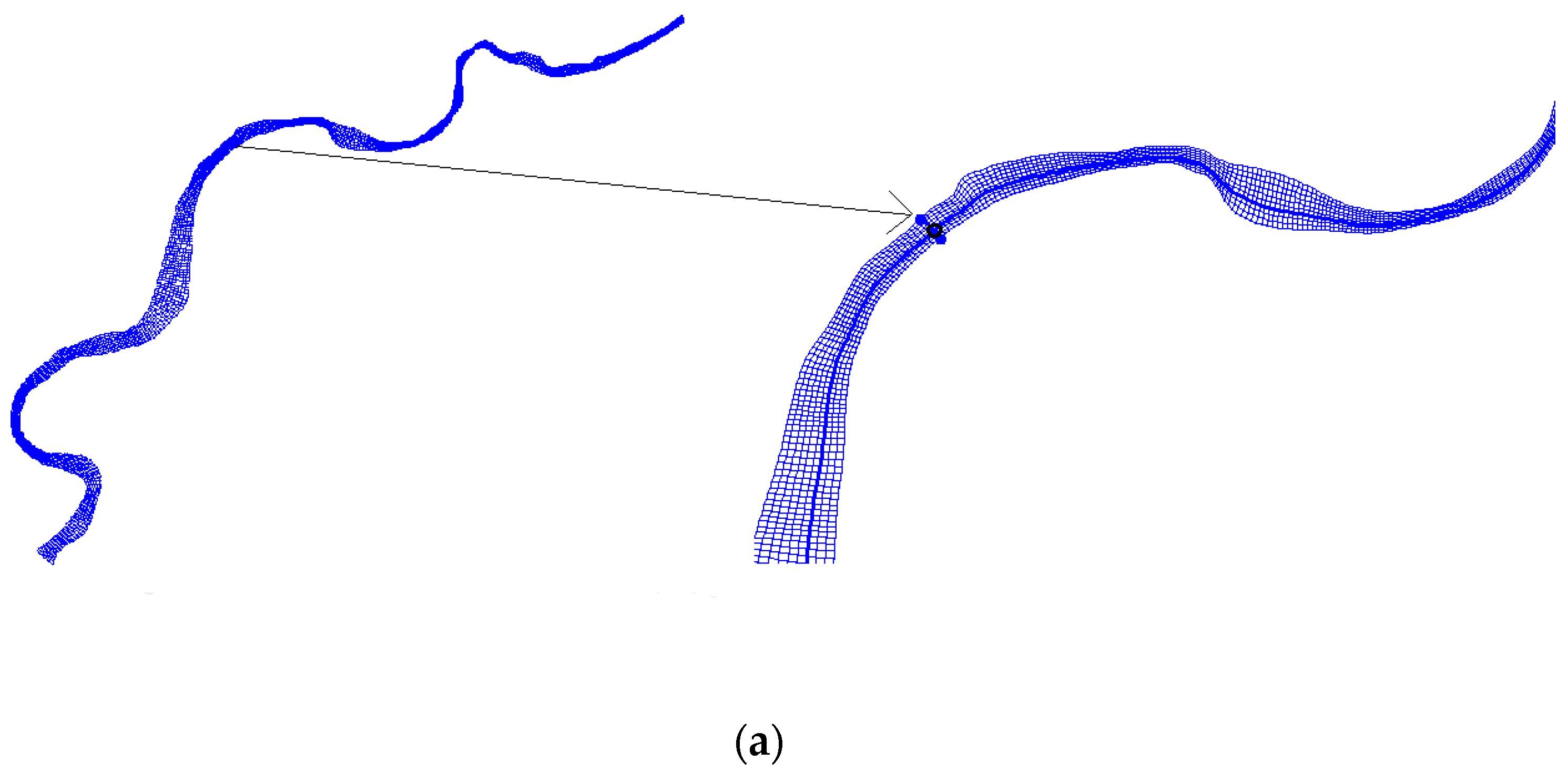
3.1. Hydrodynamic Model Setup

The Delft3D flow module was used for the hydrodynamic simulation. The hydrodynamic grid comprises 604 and 10 indices in M and N directions. The two open boundaries were upstream of Karnafuli and downstream of the estuary. The secondary bathymetry data of the river were used in the model setup in association with the field bathymetry survey (Figure 3 and Figure 4). Thus, the 3D model for a river section comprises three equally distributed layers. The upstream boundary condition was flow time series, and the downstream boundary was water level time series. The continuous model simulation was carried out during the study with a 1 min time step.

3.2. Water Quality Model Setup

The Delft3D-WAQ module has been applied here. This module is based on the 3D advection–diffusion equations and an extensive water quality library of interrelated source and sinks terms to represent water quality processes [39]. A water quality model is usually a mass balance for the pollutants or state variables necessary to describe the associated issues as:
M t = a d v e c t i o n + d i s p e r s i o n + s o u r c e
The advective transport through the domain area is related to the surface area, velocity, and concentration of the substances:
T x 0 A = ν x 0 × A × C x 0
where,
  • T x 0 A = Advective transport
  • ν x 0 = Velocity at x = x0
  • A = Surface area at x = x0
  • C x 0 = Concentration at x = x0
In terms of dispersive transport, the concentration gradient is a proportional factor:
T x 0 D = D x 0 × A × C x
where,
  • T x 0 D = Dispersive transport at x = x0
  • D x 0 = Dispersion co-efficient at x = x0
  • A = Surface area at x = x0
  • C   x = Concentration gradient at x = x0
Finally, the source transport is directly related to the discharge of the source. If the discharge is positive Q s r c > 0, then,
T s r c = Q s r c × C s r c
If Q s r c < 0,
T s r c = Q s r c × C i
where Ci represents the concentration in the receiving water quality segment, this means a scenario of water withdrawal.

3.3. Spatial and Temporal Analyses

On the contrary, points farther away from an output pixel reach the lowest weights. Greater importance was given to points close to an output pixel than to points farther away. The output pixel values are the weighted averages of input point values [40]. The IDW method is based on Equation (6).
X * = w 1 x 1 + w 2 x 2 + w 3 x 3   + + w n x n w 1 + w 2 + w 3 + + w n
w i = 1 d i x
where,
  • X* is the unknown value at a location to be determined.
  • x is the known point value.
  • w is the weight.
Unknown values in the IDW interpolation at X positions could be found from sampling points 1, 2, 3, and 4, with the distances to the X point being d1x, d2x, d3x, and d4x, respectively. The respective weight for each known value was computed by adopting Equation (7). The unknown value at position X was determined by assuming Equation (6) in the GIS environment.

3.4. Habitat Suitability Criteria (HSC) in PHABSIM

PHABSIM integrates biological information for habitat modeling purposes by using Habitat Suitability Criteria (HSC) (sometimes referred to as suitability-of-use criteria) within the various habitat models. PHABSIM deals with the specifics of HSC development. However, there are multiple species for which HSC should be entered and manipulated within PHABSIM. In PHABSIM, HSC data are created, edited, and stored. These data contain the HSC coordinate data for species and life stages: depth, velocity, and temperature. The required velocity profile of sampling points was prepared. For example, a sample profile at stations #45 and #50 are shown in Figure 5. HSCs for a particular species and life stage are typically grouped into four HSC data, representing the relationships between depth, velocity, temperature, and channel index and their corresponding suitability values. Habitat suitability indices for the three stages, i.e., fry, Juvenile, and adult life stages of Labeo rohita were prepared following Akter and Tanim (2018), and Figure 6 represents the adult stage.

3.5. Model Validation

Three different stations from the study area were selected as model validation points from the upstream and downstream portions of the river. The model outcome and observed three values were examined to validate the model’s prediction of oxygen distribution (Table 1).
The field data observed that the upstream portion of the river contains significant DO to decompose microorganisms. Both stations on the upstream site (#48 and #54) showed a higher DO concentration value than the BOD5. On the other hand, the downstream profile of the river shows the opposite scenario. Due to unplanned industrial waste disposal and pollution, the DO is significantly lower than the BOD5 and possibly leads to bacteria and other microorganisms in that portion. The model output shows a similar scenario. The model prediction is close to the observed value for BOD5 and DO in these three stations.
In contrast, the COD value from the model shows lower accuracy than the other two parameters. The overall model outcome from three different constituents for these three stations offers a promising statistical performance with the observed data (Table 2). However, the COD value shows higher fluctuation than the field observed value. The overall model simulated values reasonably match the field and laboratory-tested values (Table 2).

4. Results

4.1. Field Test

The other parameters, i.e., pH, electroconductivity, and TDS, showed a linear pattern (Table 3). Therefore, a linear interpolation was applied to map the river water quality parameter distribution throughout the Karnafuli River.

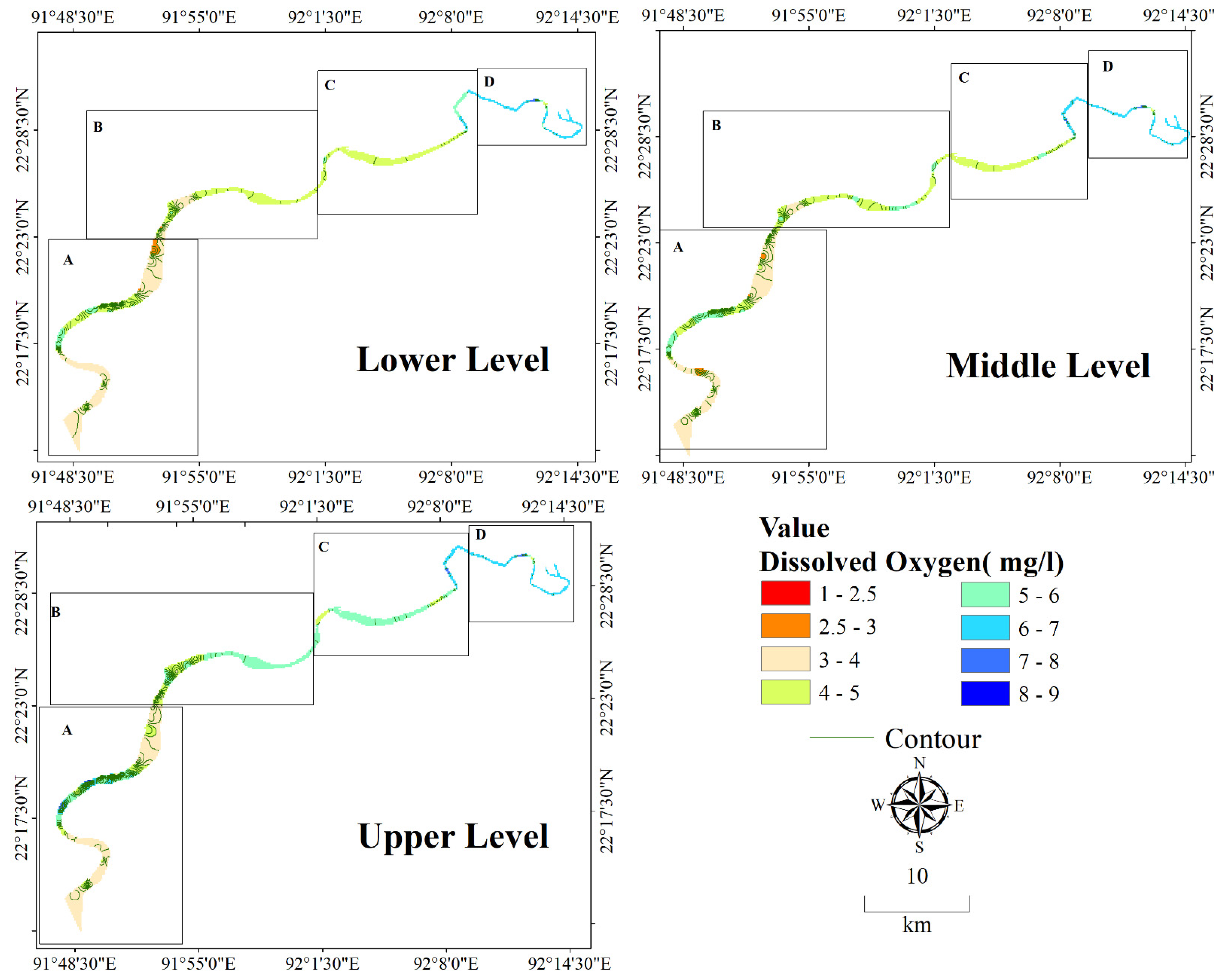
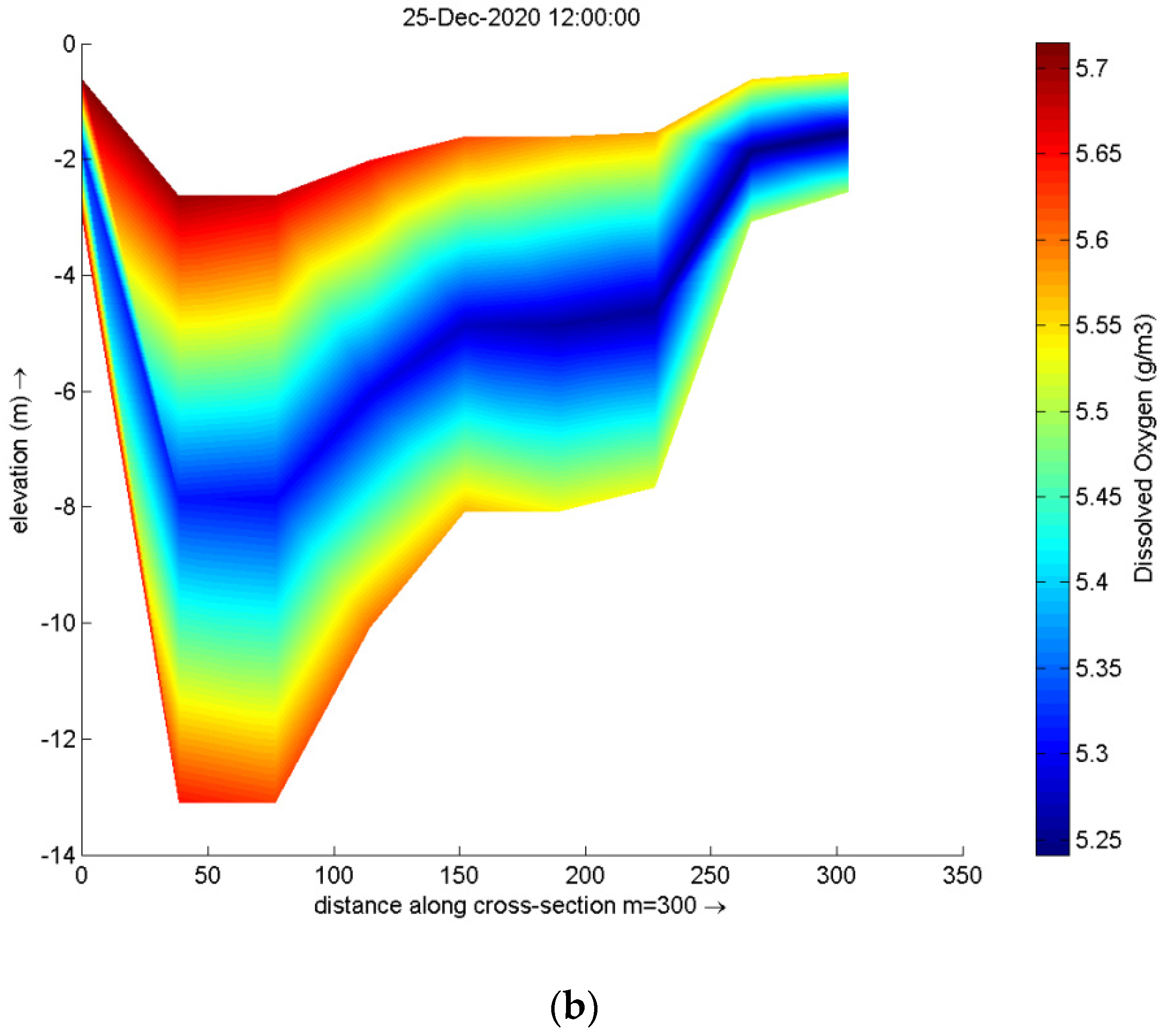
4.2. Spatial Variations of Dissolved Oxygen

Spatial variations in DO (i.e., average value for the upper, middle, and lower levels) were presented using data for the studied period. In the river estuary, DO remained saturated above 3.5 mg/L. The highest value (i.e., 8.5 mg/L) was recorded upstream, i.e., from Kaptai (92°13′57.40″ E, 22°29′36.86″ N) to Lichu Bagan Feri Ghat (92°7′50.60″ E, 22°27′53.94″ N), and decreases toward 3 mg/L. Seven locations (i.e., #6, #7, #8, #9, #10, #11#13, and #17) were found with a lower DO value within the range of 3–3.5 mg/L, and the lowest DO value of 3.1 mg/L was found at the Karnafuli new fish market (91°51′1.10″ E, 22°19′41.37″ N). Around 51% of samples showed DO levels within the range of 2.5–5 mg/L, and 39% of water samples showed DO levels within the range of 6.5–7 mg/L (Figure 7). Here the river is demonstrated into four parts based on riverside industrial development: Riverside “A” is more occupied with industrial activity than other riverside areas. Maximum Heavy industries are located at this portion of the river. Riverside “B” is less developed than Riverside “A” with industrial activity but more than others (Figure 7). Riverside “C” is mainly occupied by settlements and industry hardly exists here (Figure 7). The bank of the Riverside “D” is maximum covered with vegetation (Figure 7). A close relation was observed with the model simulation (Table 1).

4.3. Temporal Variations of Dissolved Oxygen
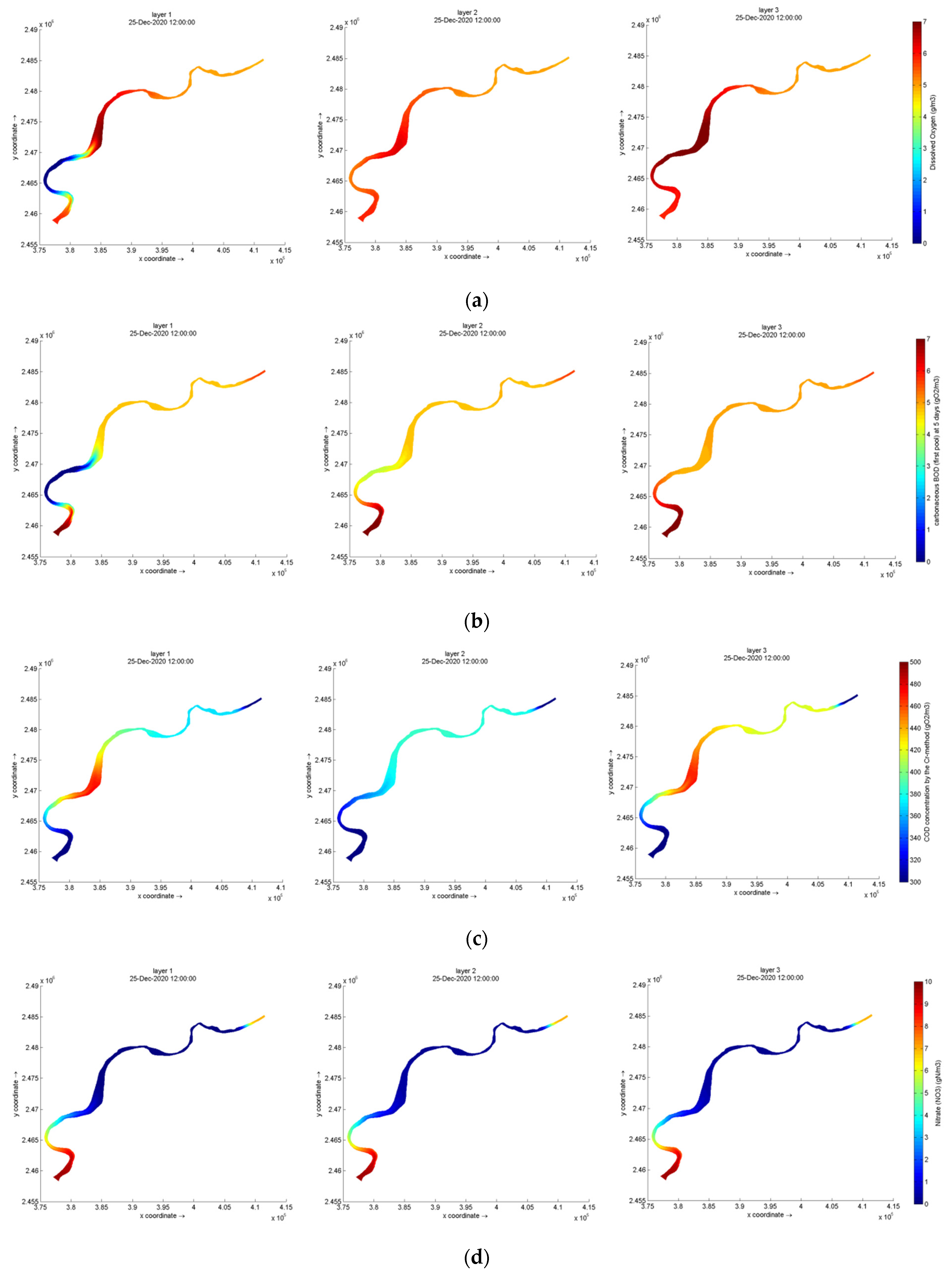
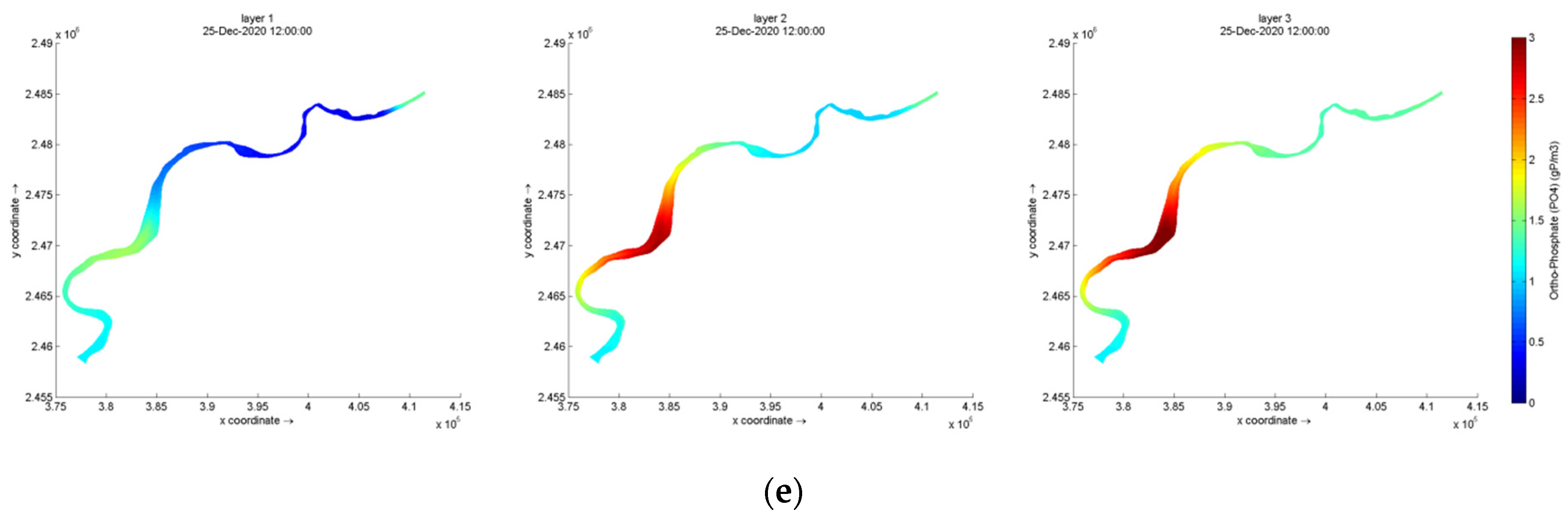
Temporal variations are based on the long-term time series. In the dry season, DO at the lower level of water depth fluctuated between 3.4 and 3.6 mg/L, then 3.4 to 4 mg/L (at the middle level) and 3.6 to 4 mg/L (the upper level) at the Karnafuli estuaries (#17). In the Navy officer’s colony point (#16), DO ranged from 3.4 to 3.6 mg/L (lower level), from 3.6 to 3.8 mg/L (middle level), and from 3.8 to 4 mg/L (upper level). In the Karnafuli new fish market (#11), DO was found as 4–5 mg/L (lower level), 4.6 to 5 mg/L (middle level), and 4 to 4.2 mg/L (upper level). In the Kalurghat heavy industrial area (#6), DO was recorded from 1.8 to 2.8 mg/L (lower level), 2 to 2.8 mg/L (middle), and 3.2 to 3.8 mg/L (upper level) (Figure 8). DO levels of 3 mg/L are generally considered very low and an issue in a river, and values of 2 or below are supposed to be highly problematic for aquatic life. The implications of this DO for the fish of interest are of great concern to the Kalurghat heavy industrial area (#6).
The upstream profile of the river shows an almost neutral and sometimes slightly alkaline pH value, while the downstream of the river’s pH is acidic. The industrial influence of different industries might influence the pH factor downstream of the river. Both electroconductivity and TDS values are much higher in the downstream zone of the river than in the upstream zone. The industries downstream can cause this higher value of solid particles in downstream water (Table 2).

4.4. Model Outcome

In terms of oxygen demand and DO, the heavy industrial area of Kalurghat possesses a higher concentration of DO in the water. DO is almost constant throughout the reach (Figure 9), except in the second bending portion near the estuary, where the concentration is nil near the industrial area. Figure 9a–c describe the scenario of DO, BOD5, and COD, respectively.
Figure 9b,c indicate that BOD5 and COD are maintaining an almost reverse relation. BOD5 was rather lower in the industrial area of the study section, where COD kept much higher values in this zone. Thus, microorganisms and aquatic plants or animals may be fewer in this zone. Still, industrial wastes containing a higher concentration of phosphorus, calcium, and sodium-ion need a higher concentration of oxygen to neutralize them. Additionally, nitrate concentration is much higher in the estuary and the adjacent portion (Figure 9d). The salt element from the seawater makes this portion too salty, with a higher concentration of nitrate ions from the nitrate salt. The rest of the study area possesses a lower level of nitrate ions (Figure 9d).
On the other hand, phosphate ions are not persistent in the estuary area (Figure 9e). A higher phosphate concentration can be observed near the industrial zone and upstream in the upper portion. The rest of the study area has a lower concentration of phosphate ions. Industrial wastes may influence the rising of phosphate ions. The parameter’s cross-section-wise distribution could be analyzed through this model as it has rendered a 3D simulation. Usually, a higher parameter concentration existed on the section’s bottom surface except for DO. The topmost surface of the section contains the lowest concentration; with the increase in depth, the concentration tends to increase.

4.5. Tidal Influence

The cross section for sampling point #47 and the river section and segment #7 in Figure 10 were carefully investigated to understand the tidal influence.
The DO concentration remains high for both the top and bottom portions of a cross section (Figure 10b). Still, DO possesses a lower concentration in the middle of a cross section. A possible explanation of this phenomenon is that the upper portion of the river has direct contact with air. Thus, the maximum amount can consume more oxygen than the middle portion. On the other hand, microorganisms, plants, and different aquatic life in the bottom section make a higher concentration of DO in the water.
The tidal effects are visible for all parameters that have been analyzed. The concentration varies with the flow pattern. The concentration moves upward during the high tide period and downward during the low tide period. The net tidal effect for every parameter has also been achieved for each cycle. The industrial influence on different water quality parameters can be easily observed for three zones (Table 4).

4.6. Habitat Modeling

Habitat Suitability Criteria (HSC) produce a measure of available physical habitats as a discharge function in the habitat modeling process. The general theory behind the habitat modeling programs within PHABSIM is based on the assumption that aquatic species will react to changes in the hydraulic environment. These changes are simulated for each cell in a defined stream reach. The stream reach simulation takes the form of a multi-dimensional matrix of the calculated surface areas of a stream having different combinations of hydraulic parameters (i.e., depth, velocity, and channel index). The depth and velocity for each cell in the PHABSIM were obtained from the Delft3D simulation. Depth and velocity attributes vary with simulated changes in discharge, causing changes in the amount and quality of the available habitat. The end product of the habitat modeling is a function of the discharge. The 3D simulated habitat plan describes the Labeo rohita habitat as suitable for the river’s temperature and relatively less urbanized portions (Figure 11). A details observation in the next phase of this work should involve a zoologist.

5. Conclusions

This study aimed to assess fish habitat suitability in a data-scarce river, the Karnafuli River. Due to increased urbanization and industrialization in the river basin, water quality and quantity seem to be a great concern of this river. This study predicts the water quality distribution over the Karnafuli River through a numerical simulation and then validates the prediction using field observation and satellite image analysis. Delft3D water quality module is a widely used numerical model applied in this study. The dry period simulation shows the spatial variation of different water quality parameters of the river. With the 3D output of the simulation, this study analyzed the layer-wise distribution of the various parameters. The intensive field survey suggested that the pollutants and industry wastes threaten the water quality downstream and near the Kalurghat area. The model simulation could replicate satellite image analysis data and field observations. The tidal effect on the river for water quality distribution was visible from the simulation. The DO concentration moves upward during the high tide period and downward during the low tide period. The model is expected to explore the water quality distribution, variation in different seasons, and flow requirements for future research. At the same time, the upstream portion of the river maintains a healthy environment for Rohu fish for their entire life stage. This habitat–discharge relationship is the basis of other fishery and recreation management analyses. This study envisaged the future application of habitat suitability assessments with intensive primary sampling for laboratory tests for this river and other rivers.

Author Contributions

Authors: A.A., M.R.T. and A.D. Conceptualization, A.A.; Model setup, M.R.T. and A.D.; Formal analysis, M.R.T., Supervision—A.A. Writing—initial draft preparation, M.R.T. and A.D.; Writing—review and editing, A.A. and M.R.T. All authors have read and agreed to the published version of the manuscript.

Funding

The Department of Civil Engineering funded this study at Chittagong University of Engineering and +Technology (CUET), Bangladesh for conducting a project titled Application of Eco-hydraulic Model cascades on the selected Rivers, CUET/DRE/2018-19/CE/028.

Informed Consent Statement

Not applicable.

Acknowledgments

The Department of Civil Engineering funded this study at Chittagong University of Engineering and Technology (CUET), Bangladesh for conducting a project titled Application of Eco-hydraulic Model cascades on the selected Rivers, CUET/DRE/2018-19/CE/028). Appreciation goes to the Department of Civil Engineering due to laboratory support and data collection supported by daily labor. Logistic support from the BWDB is also appreciated.

Conflicts of Interest

The authors declare that they have no known competing financial interests or personal relationships that could influence the work reported in this paper.

References

  1. Isiuku, B.O.; Enyoh, C.E. Pollution and health risks assessment of nitrate and phosphate concentrations in water bodies in South Eastern, Nigeria. Environ. Adv. 2020, 2, 100018. [Google Scholar] [CrossRef]
  2. Jouanneau, S.; Recoules, L.; Durand, M.J.; Boukabache, A.; Picot, V.; Primault, Y.; Lakel, A.; Sengelin, M.; Barillon, B.; Thouand, G. ScienceDirect Methods for assessing biochemical oxygen demand (BOD): A review. Water Res. 2013, 49, 62–82. [Google Scholar] [CrossRef] [PubMed]
  3. Chen, Q.; Wu, W.; Blanckaert, K.; Ma, J.; Huang, G. Optimization of water quality monitoring network in a large river by combining measurements, a numerical model and matter-element analyses. J. Environ. Manag. 2012, 110, 116–124. [Google Scholar] [CrossRef] [PubMed] [Green Version]
  4. Ali, M.M.; Ali, M.L.; Proshad, R.; Islam, S.; Rahman, Z.; Kormoker, T. Assessment of Trace Elements in the Demersal Fishes of a Coastal River in Bangladesh: A Public Health Concern. Thalassas 2020, 36, 641–655. [Google Scholar] [CrossRef]
  5. Webb, J.H.; Gibbins, C.N.; Moir, H.; Soulsby, C. Flow requirements of spawning atlantic salmon in an upland stream: Implications for water-resource management. Water Environ. J. 2001, 15, 1–8. [Google Scholar] [CrossRef]
  6. Crisp, D.T.; Carling, P.A. Observations on siting, dimensions and structure of salmonid redds. J. Fish Biol. 1989, 34, 119–134. [Google Scholar] [CrossRef]
  7. Freeman, M.C.; Bowen, Z.H.; Bovee, K.E.N.D.; Irwin, E.R. Flow and Habitat Effects on Juvenile Fish Abundance in Natural and Altered Flow Regimes. Ecol. Appl. 2001, 11, 179–190. [Google Scholar] [CrossRef]
  8. Moir, H.J.; Gibbins, C.N.; Soulsby, C.; Webb, J. Linking channel geomorphic characteristics to spatial patterns of spawning activity and discharge use by Atlantic salmon (Salmo salar L.). Geomorphology 2004, 60, 21–35. [Google Scholar] [CrossRef]
  9. Acreman, E. Evaluation of the river Wey restoration project using the Physical HABitat SIMuation (PHABSIM) model. In Proceedings of the 31st MAFF Conference of River and Coastal Engineers, London, UK, 3–5 July 1996; Keele Universit: Keele, UK, 1996. [Google Scholar]
  10. Shan, C.; Guo, H.; Dong, Z.; Liu, L.; Lu, D.; Hu, J.; Feng, Y. Study on the river habitat quality in Luanhe based on the eco-hydrodynamic model. Ecol. Indic. 2022, 142, 109262. [Google Scholar] [CrossRef]
  11. Strevens, A.P. Impacts of groundwater abstraction on the trout fishery of the River Piddle, Dorset; and an approach to their alleviation. Hydrol. Process. 1999, 13, 487–496. [Google Scholar] [CrossRef]
  12. Johnson, I.W.; Elliott, C.R.N.; Gustard, A. Modelling the effect of groundwater abstraction on salmonid habitat availability in the river Allen, Dorset, England. Regul. Rivers Res. Manag. 1995, 10, 229–238. [Google Scholar] [CrossRef]
  13. Gibbins, C.N.; Acornley, R.M. Salmonid habitat modelling studies and their contribution to the development of an ecologically acceptable release policy for Kielder Reservoir, North-east England. Regul. Rivers Res. Manag. 2000, 16, 203–224. [Google Scholar] [CrossRef]
  14. Stamou, A.I. Improving the numerical modeling of river water quality by using high order difference schemes. Water Res. 1992, 26, 1563–1570. [Google Scholar] [CrossRef]
  15. Thongtha, K. Numerical Simulations of Water Quality Measurement Model in an Opened-Closed Reservoir with Contaminant. Int. J. Differ. Equ. 2018, 2018, 1343541. Available online: https://www.hindawi.com/journals/ijde/2018/1343541/ (accessed on 29 July 2022). [CrossRef]
  16. Ma, Y.; Tie, Z.; Zhou, M.; Wang, N.; Cao, X.; Xie, Y. Accurate Determination of Low-level Chemical Oxygen Demand Using a Multistep Chemical Oxidation Digestion Process for Treating Drinking Water Samples. Anal. Methods 2016, 8, 3839–3846. [Google Scholar] [CrossRef]
  17. Beyhan, M. Hydrodynamic and Water Quality Modeling of Lake Egirdir. CLEAN Soil Air Water 2014, 42, 1573–1582. [Google Scholar] [CrossRef]
  18. Delft3D. 3D/2D Modelling Suite for Integral Water Solutions; Delft3D: Delft, The Netherlands, 2020. [Google Scholar]
  19. Deltares. D-Water Quality; Deltares: Delft, The Netherlands, 2014. [Google Scholar]
  20. Bovee KD Development and Application of Habitat Suitability Criteria for Use in the Instream Flow Incremental Methodology. US Fish Wildl. Serv. 1998, 2, 1535. [CrossRef]
  21. Tharme, R.E. A global perspective on environmental flow assessment: Emerging trends in the development and application of environmental flow methodologies for rivers. River Res. Appl. 2003, 19, 397–441. [Google Scholar] [CrossRef]
  22. Boavida, I.; Santos, J.M.; Katopodis, C.; Ferreira, M.T.; Pinheiro, A. Uncertainty in predicting the fish-response to two-dimensional habitat modeling using field data. RIVER Res. Appl. 2012, 2, 1535. [Google Scholar] [CrossRef]
  23. Luo, P.; He, B.; Takara, K.; Xiong, Y.E.; Nover, D. Historical assessment of Chinese and Japanese flood management policies and implications for managing future floods. Environ. Sci. Policy 2015, 48, 265–277. [Google Scholar] [CrossRef]
  24. Baker, E.A.; Coon, T.G.; Baker, E.A.; Coon, T.G. Development and Evaluation of Alternative Habitat Suitability Criteria for Brook Trout. Trans. Am. Fish. Soc. 2016, 8487, 1573–1582. [Google Scholar] [CrossRef]
  25. Zhang, H.; Wang, C.Y.; Wu, J.; Du, H.; Wei, Q.W.; Kang, M. Physical habitat assessment of a remaining high- biodiversity reach of the upper yangtze river. Appl. Ecol. Environ. Res. 2016, 14, 129–143. [Google Scholar] [CrossRef]
  26. Santos, J.M.; Boavida, I.; Branco, P. Structural microhabitat use by endemic cyprinids in a Mediterranean-type river: Implications for restoration practices. Aquat. Conserv. Mar. Freshw. Ecosyst. 2018, 28, 26–36. [Google Scholar] [CrossRef]
  27. Hearne, J.; Johnson, I.; Armitage, P. Determination of ecologically acceptable flows in rivers with seasonal changes in the density of macrophyte. Regul. Rivers Res. Manag. 2002, 9, 177–184. [Google Scholar] [CrossRef]
  28. Hatfield, T.; Bruce, J. Predicting Salmonid Habitat–Flow Relationships for Streams from Western North America. N. Am. J. Fish. Manag. 2000, 20, 1029–1032. [Google Scholar] [CrossRef]
  29. Beland, K.F.; Jordan, R.M.; Meister, A.L. Water Depth and Velocity Preferences of Spawning Atlantic Salmon in Maine Rivers. N. Am. J. Fish. Manag. 1982, 2, 11–13. [Google Scholar] [CrossRef]
  30. Gore, J.A.; Crawford, D.J.; Addison, D.S. An analysis of artificial riffles and enhancement of benthic community diversity by physical habitat simulation (PHABSIM) and direct observation. Regul. Rivers Res. Manag. 1998, 14, 69–77. [Google Scholar] [CrossRef]
  31. ADB. Institutional Strengthening of Chittagong Port Authority in Environmental Managemen; ADB: Dhaka, Bangladesh, 2004. [Google Scholar]
  32. Uddin, M.J.; Parveen, Z. Status of heavy metals in water and sediments of canals and rivers around the Dhaka city of Bangladesh and their subsequent transfer to crops. Adv. Plants Agric. Res. 2016, 5, 593–601. [Google Scholar] [CrossRef]
  33. Samad, R.B. Urbanization and Urban Growth Dynamics: A Study on Chittagong City. J. Bangladesh Inst. Plan. 2016, 8, 167–174. [Google Scholar]
  34. Akter, A.; Tanim, A.H. Salinity Distribution in River Network of a Partially Mixed Estuary. J. Waterw. Port Coast. Ocean Eng. 2021, 147, 1–16. [Google Scholar] [CrossRef]
  35. Tabrez, S.; Zughaibi, T.A.; Javed, M. Water quality index, Labeo rohita, and Eichhornia crassipes: Suitable bio-indicators of river water pollution. Saudi J. Biol. Sci. 2022, 29, 75–82. [Google Scholar] [CrossRef] [PubMed]
  36. APHA, Standard methods for the examination of water and wastewater. J. Tuberc. Res. 1999, 4, 111–121. [CrossRef] [Green Version]
  37. Bajpai, P. Environmental Impact 15.1; Biermanns Handbook of Pulp and Paper; Elsvier: Amsterdam, The Netherlands, 2018; pp. 325–348. ISBN 9780128142387. [Google Scholar]
  38. Mckenzie, S.W. Five-day biochemical oxygen demand 7.0. US Geol. Surv. 2003, 7, 1–21. [Google Scholar]
  39. Hok-Shing, L. The Application of Numerical Modelling in Managing Our Water Environment; Environmental Protection Officer, Environmental Protection Department, 2007. Available online: https://www.science.gov.hk/paper/EPD_HSLee.pdf (accessed on 29 July 2022).
  40. Chakraborty, A.; Sain, M.M.; Kortschot, M.T.; Ghosh, S.B. Modeling energy consumption for the generation of microfibres from bleached kraft pulp fibres in a PFI mill. BioResources 2007, 2, 210–222. [Google Scholar] [CrossRef]
Figure 1. Adopted methodology.
Hydrology 09 00173 g001
Figure 2. (a) Study area. (b) Industrial zone in Karnafuli River and sampling points.
Hydrology 09 00173 g002aHydrology 09 00173 g002b
Figure 3. Hydrodynamic grid of the study area.
Hydrology 09 00173 g003
Figure 4. Bathymetry map of the study area.
Hydrology 09 00173 g004
Figure 5. Velocity profile of sampling stations #45 and #50.
Hydrology 09 00173 g005
Figure 6. Habitat suitability indices for the different adult stages of Labeo rohita (Rohu fish) (after [34].
Hydrology 09 00173 g006
Figure 7. Spatial distribution of dissolved oxygen (Karnafuli River) for better visualization subfigures A-D has been added.
Hydrology 09 00173 g007
Figure 8. Dissolved oxygen level at different water depths (Dry season) for better visualization subfigures A–D has been added.
Hydrology 09 00173 g008
Figure 9. (a) Dissolved oxygen concentration throughout the study area. (b) Biochemical oxygen demand throughout the study area. (c) Chemical oxygen demand throughout the study area. (d) Nitrate-ion concentration throughout the study area. (e) Phosphate-ion concentration throughout the study area.
Hydrology 09 00173 g009aHydrology 09 00173 g009b
Figure 10. (a) Location of the cross section for sampling point #47. (b) Dissolved oxygen concentration for sampling point #47.
Hydrology 09 00173 g010aHydrology 09 00173 g010b
Figure 11. Labeo rohita (Rohu fish) adult life stage 3D habitat plan view.
Hydrology 09 00173 g011
Table 1. Model prediction and observed values for different stations.
Station IDStation NameConstituentField ObservedDelft 3D
Simulation
Spatial
Analysis
#54MohraBOD5 (mg/L)3.64.23.9
COD (mg/L)416409425
DO (mg/L)6.445.84.8
#48Halda-Karnafuli colfluenceBOD5 (mg/L)5.14.45.5
COD (mg/L)352405390
DO (mg/L)6.125.95.5
#89EstuaryBOD5 (mg/L)6.156.5
COD (mg/L)400320386
DO (mg/L)3.643.0
Table 2. Statistical performance of the overall model outcomes compared to the field observations.
Performance Statistics
1Efficiency Index (EI.)0.97
2Standard deviation of observed data, sx192.81
Standard deviation of model predicted data, sy188.25
3Root Mean Square Error (RMSE)32.08
4Mean Absolute Error (MAE)15.97
5Ratio Mean Square Error Method (RMSEM)0.24
6Mean Percentage Error (MPE)2.86
7Mean Absolute Percentage Error (MAPE)12.38
8Correlation Coefficient (R)0.98
9Coefficient of Determination (R2)0.97
Table 3. Observed water quality parameters (mean ± standard deviation) in different locations of the Karnafuli River.
StationStation IDpHElectroconductivity
μS/cm
TDS
(mg/L)
Kalurghat Halda Mohona48Upper7.89 ± 0.19Upper0.54 ± 0.60Upper274.27 ± 244.72
Middle7.51 ± 0.97Middle0.5 ± 0.33Middle181.2 ± 35.75
Lower8.19 ± 0.46Lower0.14 ± 0.03Lower222.16 ± 57.81
Kalurghat Bridge49Upper7.58 ± 0.86Upper0.74 ± 0.42Upper363.40 ± 342.60
Middle8.45 ± 0.90Middle0.48 ± 0.34Middle338.2 ± 17.22
Lower7.28 ± 1.80Lower0.31 ± 0.09Lower264.53 ± 11.75
Kalurghat Heavy Industrial Area51Upper7.64 ± 0.69Upper0.62 ± 0.84Upper674.53 ± 852.60
Middle8.14 ± 0.71Middle0.54 ± 0.17Middle300.2 ± 76.98
Lower7.88 ± 0.3Lower0.3 ± 0.19Lower4186.43 ± 6749.43
Mohra54Upper7.79 ± 0.81Upper0.84 ± 0.99Upper744.03 ± 905.41
Middle8.31 ± 0.99Middle0.79 ± 0.70Middle518.63 ± 333.73
Lower8.1 ± 0.68Lower0.9 ± 0.82Lower437 ± 268.49
Baxir Hut59Upper7.61 ± 0.32Upper1.32 ± 1.32Upper1327.83 ± 984.74
Middle8.10 ± 0.86Middle2.63 ± 2.77Middle713.16 ± 172.26
Lower6.67 ± 1.35Lower3.23 ± 3.31Lower1186.4 ± 1146.39
Chaktai Wapda Ferri Ghat60Upper7.41 ± 0.19Upper3.62 ± 1.11Upper2812.20 ± 2442.41
Middle6.54 ± 1.79Middle4.49 ± 3.31Middle1711.86 ± 654.67
Lower7.32 ± 0.15Lower6.06 ± 4.07Lower3221.5 ± 1903.15
Khal (near new bridge)61Upper6.90 ± 1.21Upper4.60 ± 0.48Upper2181.77 ± 803.40
Middle7.02 ± 0.45Middle5.84 ± 4.24Middle2923.2 ± 3254.69
Lower7.38 ± 0.11Lower7.56 ± 4.32Lower2572.65 ± 915.69
Karnaphuli New Fish Market62Upper6.54 ± 1.76Upper5.43 ± 0.29Upper4624.83 ± 575.50
Middle7.13 ± 0.45Middle7.64 ± 4.00Middle5104.5 ± 2170.7
Lower7.61 ± 0.17Lower7.6 ± 4.1Lower26,581.87 ± 41193.51
Firingi Bazar Ghat67Upper6.41 ± 1.78Upper7.53 ± 1.46Upper5521.07 ± 2267.21
Middle7.77 ± 0.69Middle13.49 ± 10.51Middle20,414.4 ± 27625.08
Lower7.45 ± 0.18Lower11.84 ± 4.82Lower7362.93 ± 3010.71
Old Custom Mosque70Upper7.38 ± 0.13Upper10.72 ± 3.54Upper5284.77 ± 1827.41
Middle7.55 ± 0.27Middle13.71 ± 6.19Middle5722.2 ± 1050.02
Lower7.46 ± 0.19Lower18.71 ± 9.07Lower7631.26 ± 3413.40
Majir Ghat71Upper7.37 ± 0.22Upper11.74 ± 3.97Upper9571.77 ± 4970.81
Middle7.61 ± 0.96Middle20.23 ± 14.16Middle6571.63 ± 5804.96
Lower7.27 ± 0.115Lower23.66 ± 7.69Lower13,318.53 ± 8341.90
Saltgola Bus Stop74Upper6.81 ± 1.17Upper17.40 ± 7.45Upper7230.43 ± 6705.51
Middle7.10 ± 0.19Middle23.25 ± 13.27Middle14,573.67 ± 5878.52
Lower7.27 ± 0.27Lower26.35 ± 4.03Lower14,770.2 ± 8124.04
Navy Officers Colony Point76Upper6.94 ± 1.15Upper19.87 ± 8.63Upper16,407.10 ± 8646.90
Middle7.39 ± 0.73Middle23.6 ± 12.55Middle16,525.43 ± 9026.642
Lower7.43 ± 0.17Lower28.45 ± 4.03Lower17,749.8 ± 10063.04
Karnafuli Estuaries89Upper7.30 ± 1.02Upper20.03 ± 8.82Upper15,475.07 ± 6236.96
Middle6.46 ± 1.69Middle26.16 ± 9.36Middle19,120.1 ± 7652.73
Lower6.66 ± 0.19Lower28.25 ± 4.31Lower17,250.13 ± 8114.56
Table 4. Distribution of chemical substances in three different industrial zones.
StationBOD (mg/L)COD (mg/L)DO/E-9 (mg/L)Nitrate/100 (mg/L)Phosphate/100 (mg/L)
Upstream non-industrial zone5360510070
Kalurghat industrial zone4.54403300150
Downstream industrial zone6.53005900100
Publisher’s Note: MDPI stays neutral with regard to jurisdictional claims in published maps and institutional affiliations.

