On the Benefits of Bias Correction Techniques for Streamflow Simulation in Complex Terrain Catchments: A Case-Study for the Chitral River Basin in Pakistan

Abstract

This work evaluates the suitability of linear scaling (LS) and empirical quantile mapping (EQM) bias correction methods to generate present and future hydrometeorological variables (precipitation, temperature, and streamflow) over the Chitral River Basin, in the Hindukush region of Pakistan. In particular, LS and EQM are applied to correct the high-resolution statistically downscaled dataset, NEX-GDDP, which comprises 21 state-of-the-art general circulation models (GCMs) from the coupled model intercomparison project phase 5 (CMIP5). Raw and bias-corrected NEX-GDDP simulations are used to force the (previously calibrated and validated) HBV-light hydrological model to generate long-term (up to 2100) streamflow projections over the catchment. Our results indicate that using the raw NEX-GDDP leads to substantial errors (as compared to observations) in the mean and extreme streamflow regimes. Nevertheless, the application of LS and EQM solves these problems, yielding much more realistic and plausible streamflow projections for the XXI century.

1. Introduction

General circulation models (GCMs) are the mostly widely used tools to generate long-term projections of different climate variables, such as precipitation and temperature, on global scales. However, the spatial resolution of these GCMs is too coarse yet (around 50 km in the most recent models) [1,2], which strongly limits their usability for impact studies, which typically require local-scale information [3,4,5,6,7,8,9]. Indeed, their usefulness is especially questionable in regions with complex terrain characteristics, where most of the GCMs are not able to adequately resolve several factors directly affecting the local climate (e.g., topography, net radiation, or water vapor fluxes) [10,11,12,13].

For the particular case of hydrology, even though the coarse outputs from GCMs can be used directly in impact studies, applications at the basin and/or catchment levels normally rely on some form of downscaling (either statistical or dynamical), which allows for the better incorporation of local-scale features of relevance for the region under study, such as complex topography or sub grid processes that are not represented by the GCMs [3,4,14].

In this context, statistical downscaling (SD) aims to build empirical relationships linking the large-scale circulation (e.g., geopotential height, winds, and humidity at different vertical levels) to the local scale (e.g., precipitation at one particular site) [15,16]. Differently, dynamical downscaling (DD) is based on the use of the high-resolution regional climate model (RCMs), which is nested to the coarser GCMs over a limited area [4]. Both SD and DD are widely recognized as complementary approaches leading to overall similar results in many situations (see, e.g., [17] for a detailed discussion on this topic). Here, we use SD, which is computationally cheaper than DD.

An ensemble of 21 state-of-the-art GCMs from the fifth coupled model intercomparison project (CMIP5) have been downscaled to a high-resolution (0.25° × 0.25°) common grid and made publicly available by the National Aeronautics and Space Administration (NASA), through a product called the NASA Earth Exchange (NEX) Global Daily Downscaled Projections (GDDP) dataset [18], (https://www.nccs.nasa.gov/services/data-collections/land-based-products/nex-gddp (accessed on 20 July 2021)). This dataset (NEX-GDDP, hereafter), which is based on a SD technique known as bias-corrected spatial disaggregation (BCSD) [18,19,20,21], provides daily precipitation and the maximum and minimum temperatures globally from 1950 to 2005. NEX-GDDP has rapidly become one of the most popular datasets within the climate community, and its performance over different regions of the world has been already assessed in numerous previous studies. For instance, [22] investigated the future changes of precipitation at the local scale over China using NEX-GDDP and reported a “certain” reliability over the Han River, emphasizing the potential usefulness of this dataset for climate change impact studies at watershed scales. The author of [23] reported that, although NEX-GDDP offers potential improvements in reproducing monthly temperature and precipitation over China, it still exhibits region-dependent systematic errors. The author of [24] reported this dataset to be well in agreement with the observations on a monthly basis over southeast Asia; however, they also found significant biases, which were predominantly region-specific. The author of [25] used NEX-GDDP over India and reported the existence of some biases (e.g., significant overestimation and underestimation of temperature and precipitation, respectively). The author of [26] showed the existence of significant biases in this dataset for some regions in India.

Despite this extensive body of research, only a few studies (to-date) have focused on the assessment of the adequacy of NEX-GDDP downscaled data for hydrological applications. The present work aims to fill this gap, building on the premise that the convincing replication of historic streamflow conditions is the least of the requirements to be fulfilled by any hydrological model in which downscaled climatic data are used as inputs [20,27]. In other words, if a hydrological model is unable to replicate historic streamflow conditions in an efficient manner, it will most likely continue to perform inadequately in the future (e.g., [28,29,30]).

Moreover, note that having high-quality climate information is one of the key requirements for the assessment of long-term variations in the hydrologic cycle of a region [2]. For instance, small biases in the climate-driving variables can lead to significant changes in the dynamics of the hydrological system being studied [31]. As such, it is well-established that the direct use of GCM outputs (which typically incorporate important systematic biases) as inputs to drive the hydrological models is unreasonable and of little utility [32,33]. To overcome this issue, bias correction techniques are usually applied to improve the reliability of the raw GCM outputs [2,34].

Owing to the importance of bias correction, this work investigates the applicability of the NEX-GDDP dataset to simulate hydrometeorological conditions in Chitral River Basin (CRB), Pakistan. To do so, we first assess the biases that are present in this high-resolution dataset over this complex terrain region. Subsequently, linear scaling (LS) and empirical quantile mapping (EQM) methods are applied to correct the NEX-GDDP meteorological data that are used as inputs to a (previously calibrated and validated) hydrological model, in order to produce local streamflow projections, up to the end of the 21st century. This allows us to assess the potential impacts that different bias correction strategies may have on the projected hydrological regime of the catchment.

2. Data and Methods

2.1. Study Area and Data Description

The CRB is located in Pakistan and is one of the river basins of the Hindukush–Karakoram–Himalayan (HKH) region (Figure 1). It is characterized by complex orographic features and drains an area of more than 11,000 km², and its streamflow is predominantly fed by snow and glacier melt [35]. The river water supports domestic activities, and irrigation is dependent on it. It plays a key role in the socio-economic development of the region. Note, also, that the CRB is considered one of the most complex terrain catchments of High Mountain Asia (HMA).

Daily precipitation and temperature for the period of 1994–2012 were provided by the Pakistan Meteorological Department (PMD), and the daily streamflow data were obtained from the Surface Water Hydrology Project (SWHP) of the Water and Power Development Authority (WAPDA) in Pakistan for the same period. The digital elevation model (DEM), of 90 m resolution, from the Shuttle Radar Topographic Mission (SRTM) was retrieved from http://srtm.csi.cgiar.org (accessed on 2 February 2021) and covers the entire region of study. Finally, the NEX-GDDP dataset, which contains daily precipitation and maximum and minimum temperature values from 21 GCMs included in the CMIP5 project [18,19,20,21] was obtained from https://ds.nccs.nasa.gov/thredds/catalog/bypass/NEX-GDDP/catalog.html (accessed on 20 July 2021). These 21 GCMs have been downscaled using the bias-correction spatial disaggregation (BCSD) method [36], providing high-resolution simulations for historic (1951–2005) and future (2006–2099) periods. For the latter, two different greenhouse gas emission scenarios (representative concentration pathways (RCPs)) were considered, namely RCP 4.5 and RCP 8.5, respectively.

2.2. Hydrological Modeling

The Hydrologiska Byråns Vattenbalansavdelning (HBV) hydrological model [37,38] was used in this study. Streamflow was simulated using the modified HBV-light (version # 4.0.0.23) [39]. The input data (streamflow, precipitation, and temperature) used for hydrological modeling was sourced from hydrological and climate stations in the catchment. Once the model was fed with all the required input variables, it was calibrated using a genetic algorithm and Powell optimization (GAP; [40]). For the calibration of the HBV-light model, thirteen years were selected, 1995–2007, leaving five years, 2008–2012, for validation. The year 1994 was used as a spin-up period. However, the objective function maximizes the NSE. Even though the NSE has a quadratic nature that favors the model’s ability to simulate high flows [41], it can also approach optimum values, due to periodicity. Nonetheless, different statistical measures, including Nash–Sutcliffe efficiency (NSE), co-efficient of determination (R2), and percent bias, were used to assess the model’s performance. NSE was used as an objective function to calibrate the model. For further details about calibration and validation of HBV-light, the interested readers are referred to the following sources: [4,42,43,44].

2.3. Bias Correction

Observed precipitation and temperature are typically misrepresented by GCMs when they are evaluated at local spatial scales. Particularly, systematic biases may arise [9,45], making the application of some form of correction to adjust their raw outputs [2,46] towards the corresponding observations necessary. Here, we use two popular bias correction techniques to adjust the NEX-GDDP towards the available gauge meteorological data, namely linear scaling (LS) and empirical quantile mapping (EQM). The common period for NEX-GDDP and observations, 1995–2005, is used to this aim. Both LS and EQM are separately applied to each of the calendar months, based on daily data. That is, we built twelve independent statistical models. In all cases, the correction factors derived in the training phase for the period 1995–2005 were then applied to correct for the future simulations from NEX-GDDP for the period 2040–2100. In order to avoid the artificial skill that may arise from model overfitting, a leave-one-year-out cross-validation strategy [47] was adopted, in which each year was separately considered for testing, whilst the remaining ones were kept for fitting/calibration.

2.3.1. Linear Scaling (LS)

Linear scaling (LS) is the simplest bias correction technique and has been applied in numerous studies, with overall good results [48,49,50]. This method aims to match the mean of the simulated values with that of observed ones [50]. A multiplicative term is typically used to correct precipitation, whilst an additive term is used for temperature (Equations (1) and (2), respectively) [51].

$$p{r}_{gcm,M}^{crc}=p{r}_{gcm,M}^{raw}\ast \left(\frac{\overline{p{r}_{obs,M}}}{\overline{p{r}_{gcm,M}^{raw}}}\right), \mathrm{for} M=\{1, 2,\dots , 12\}$$

(1)

$$t{m}_{gcm,M}^{crc}=t{m}_{gcm,M}^{raw}+\left(\overline{t{m}_{obs,M}}-\overline{t{m}_{gcm,M}^{raw}}\right), \mathrm{for} M=\{1, 2,\dots , 12\}$$

(2)

where $pr$ and $tm$ stand for precipitation and temperature, M indicates the month of interest (1 stands for January, 2 for February, etc.), $gcm$ points to the NEX-GDDP data, $obs$ indicates observed station data, and $crc$ means corrected (bias).

2.3.2. Empirical Quantile Mapping (EQM)

Empirical quantile mapping (EQM) aims to adjust the simulated empirical cumulative distribution function (CDF) towards the observed one [52,53], using a number of quantiles [54]. Before adding each quantile to the observed quantile to create a revised calibrated CDF for the future period with a demonstrated climate change signal, the changes in the CDF are further rescaled, depending on the CDF during calibration or historical period [55]. Here, we use the particular implementation described in [56].

$$p{r}_{gcm,M}^{crc}=CD{F}_{obs}^{-1}\left(CD{F}_{gcm}\left(p{r}_{gcm,M}^{raw}\right)\right), \mathrm{for} M=\{1, 2,\dots , 12\}$$

(3)

$$t{m}_{gcm,M}^{crc}=CD{F}_{obs}^{-1}\left(CD{F}_{gcm}\left(t{m}_{gcm,M}^{raw}\right)\right), \mathrm{for} M=\{1, 2,\dots , 12\}$$

(4)

2.4. Assessing the Impacts of Bias Correction on Hydrometeorological Projections

In order to assess the reliability of NEX-GDDP over the region of study, we first analyzed the annual cycle of precipitation and temperature over the CRB for the reference period 1995–2005, as provided by the observations, raw, and LS- and EQM-corrected NEX-GDDP (Section 3.2).

After being calibrated, the HBV-light model was forced with (1) observed (Obs), (2) raw NEX-GDDP (raw), (3) LS bias-corrected NEX-GDDP (LS), and (4) EQM bias-corrected NEX-GDDP (EQM) precipitation and temperature data to simulate the streamflow for the same reference period, 1995–2005. We focused on mean monthly streamflow, 7-day minimum and maximum streamflow, and percentiles 10th and 90th of streamflow, and to compliment the streamflow, mean monthly precipitation and temperature were also analyzed (Section 3.2).

Afterwards, raw and LS- and EQM-corrected NEX-GDDP models were fed into HBV-light to simulate the streamflow characteristics of the CRB for the mid-future (2040–2069) and far future (2070–2099) periods, under both RCP 4.5 and RCP 8.5 emission scenarios. Again, we focused on mean monthly streamflow, 7-day minimum and maximum streamflow, 10th and 90th percentiles of streamflow, and mean monthly precipitation and temperature, which allowed us to assess the impacts of bias correction on future hydrometeorological projections (Section 3.3 and Section 3.4)

3. Results and Discussion

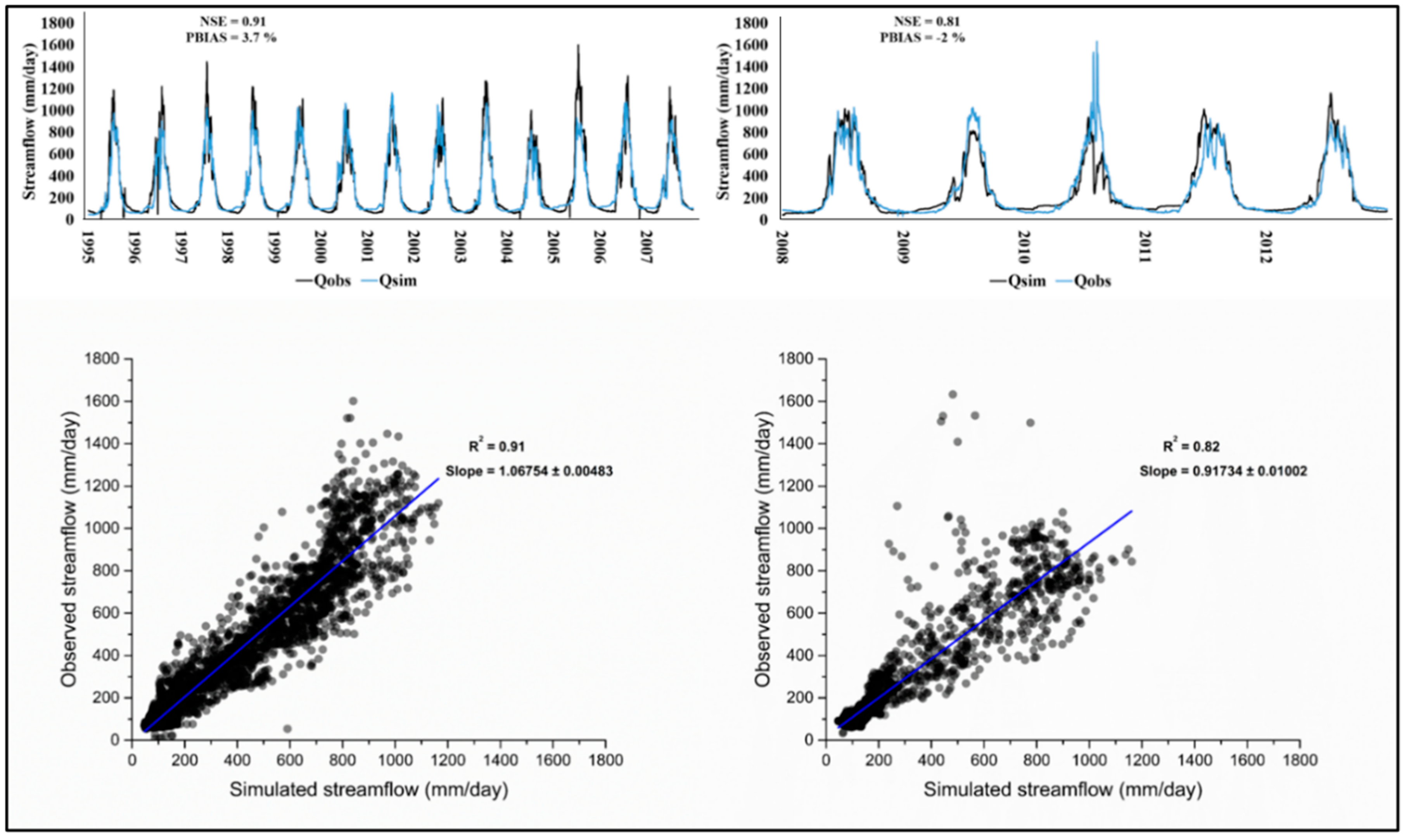
3.1. Calibration and Validation

As shown in Figure 2, the performance of the HBV-light was very good for the calibration period (1995–2007), with an NSE value of 0.91, a PBIAS of 3.7%, and an R² value of 0.91. These good results were found to be consistent for the validation period (2008–2012), reaching an NSE value of 0.81, a PBIAS of −2% and a R² value of 0.82. Overall, the HBV-light was able to accurately simulate historic streamflow over the CRB.

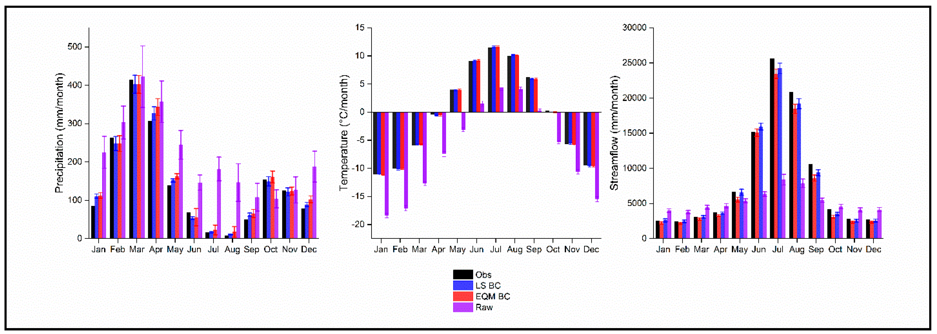
3.2. Impacts of Bias Correction on Simulated Observed Hydrometeorological Conditions

Figure 3 shows that considerable monthly biases exist between raw NEX-GDDP model outputs and observations for the reproduction of the annual precipitation cycle over the CRB. Note that the observed precipitation is substantially higher in NEX-GDDP models over the central part of the year (May to September), but also in December and January for the period 1995–2005 (left panel). However, these biases were considerably reduced in the LS- and EQM-corrected NEX-GDDP models.

The observed temperature was significantly lower in the wet period (June–September), according to the raw NEX-GDDP models, for the period 1995–2005 (center panel). Differently, the observed temperatures were substantially higher for November–April (dry and early wet season). Nevertheless, LS- and EQM-corrected NEX-GDDP provided unbiased results throughout the entire year.

Even though the raw NEX-GDDP models considered in this study are already bias-corrected and provide a high resolution, they still exhibit significant biases. One potential explanation for this negative behavior is that the BCSD is applied based on spatially aggregated reference data, which typically misrepresent important local events, especially in regions with complex topography, such as Hindukush. Therefore, to remove these biases, the above-described LS and EQM methods were applied. Both LS and EQM performed well in simulating observed precipitation and temperature; however, LS has a better impact on simulated observed precipitation than the EQM.

The HBV-light model was forced with the observed data, raw, LS-corrected and EQM-corrected NEX-GDDP data, to simulate streamflow for the reference period 1995–2005 (right panel). As compared to the observed data, the raw NEX-GDDP led to significantly lower streamflow in the wet season (from May to late September). For the rest of year, however, raw NEX-GDDP yielded higher than the observed streamflow. Nonetheless, when LS- and EQM-corrected NEX-GDDP data were used as inputs to the HBV-light model, the simulated streamflow closely resembled the observed values throughout the entire year.

Other extreme aspects, such as 7-day minimum and maximum streamflow, and 10th and 90th percentile streamflow, were also shown to be highly sensitive to the driving input data used (Figure 4). In particular, the simulations provided by the HBV-light model, when it was forced with raw NEX-GDDP data, presented substantial deviations, as compared to the observed values. Differently, the simulations driven with LS- and EQM-corrected NEX-GDDP data showed consistent similarity with the observations.

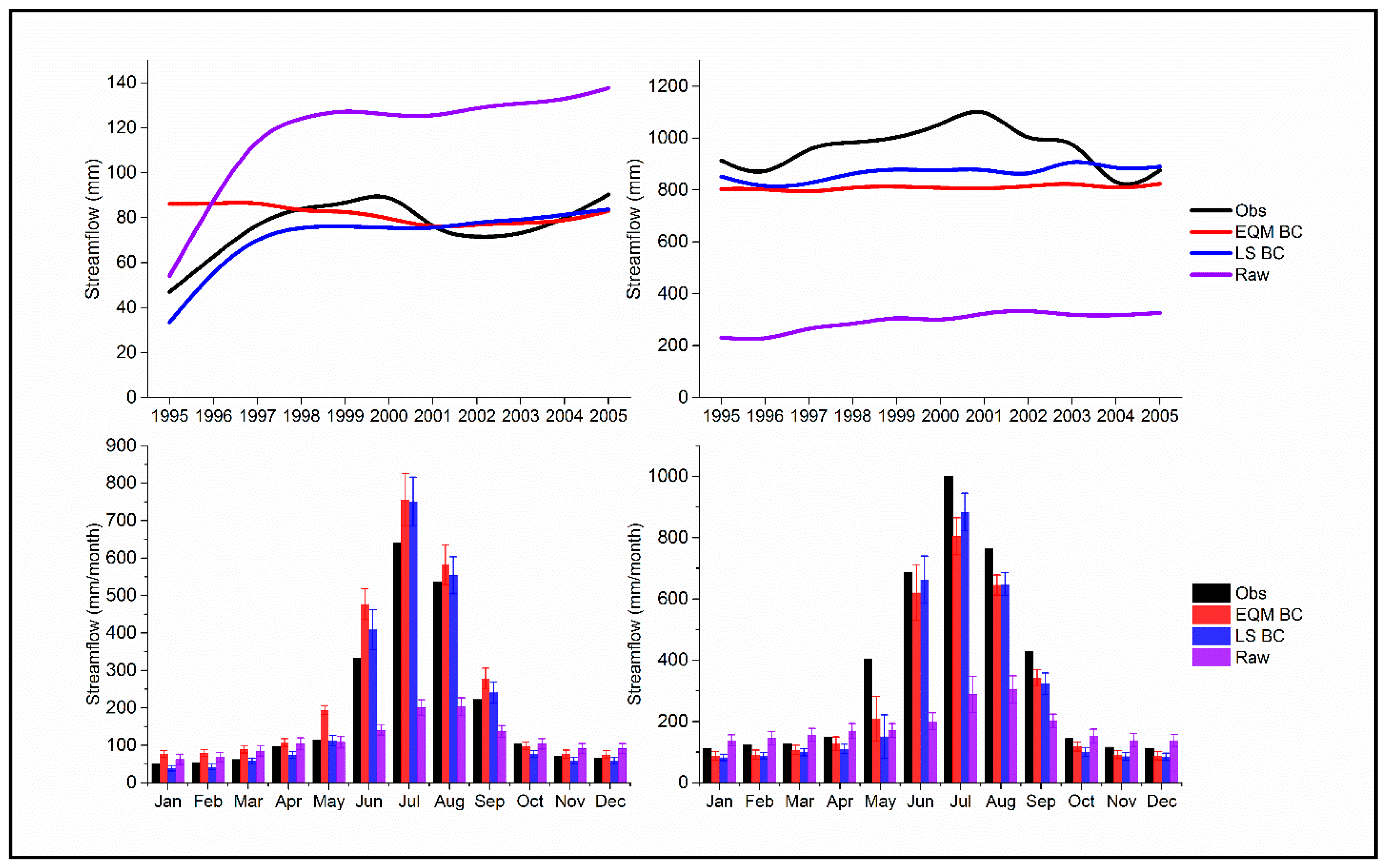
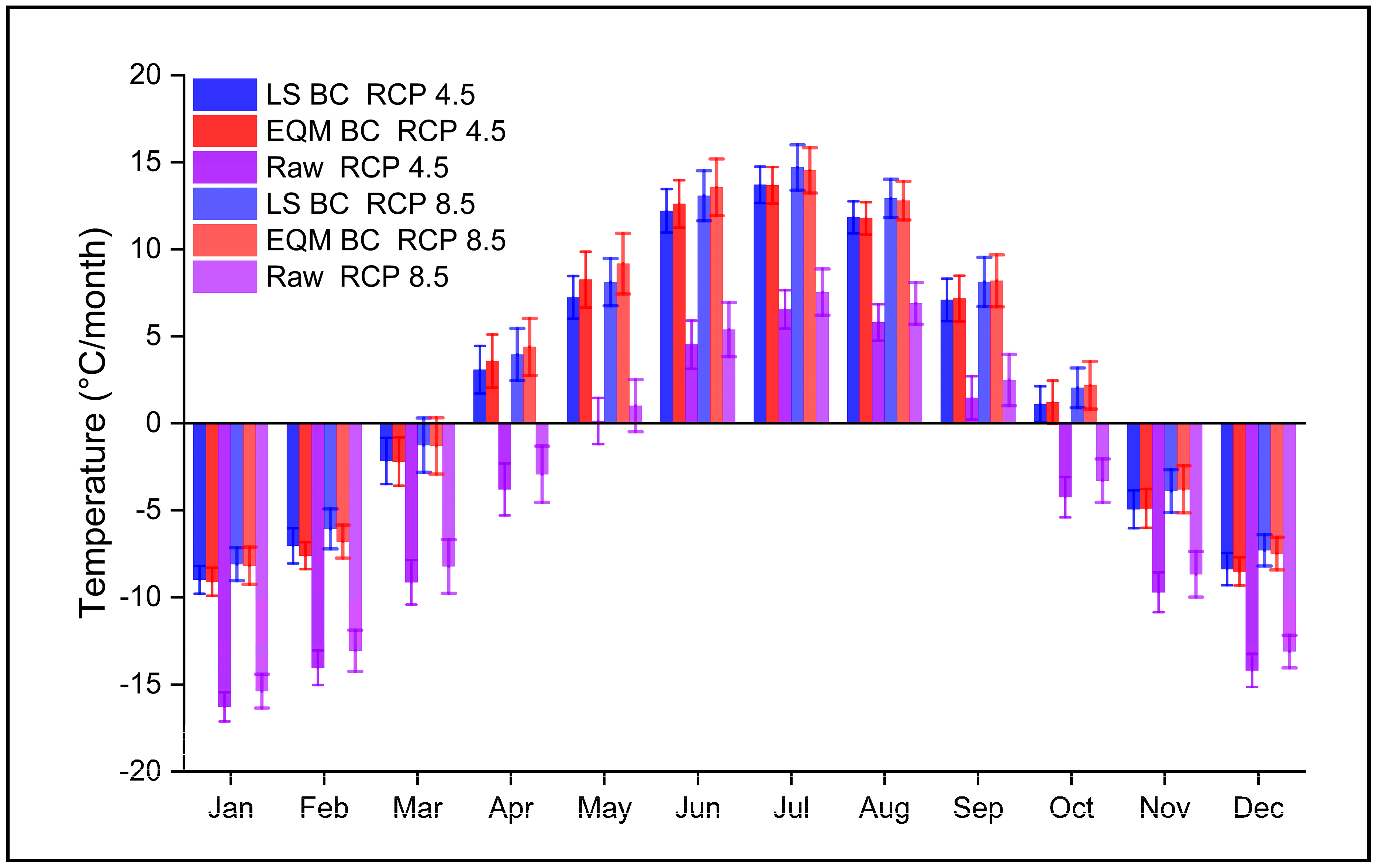
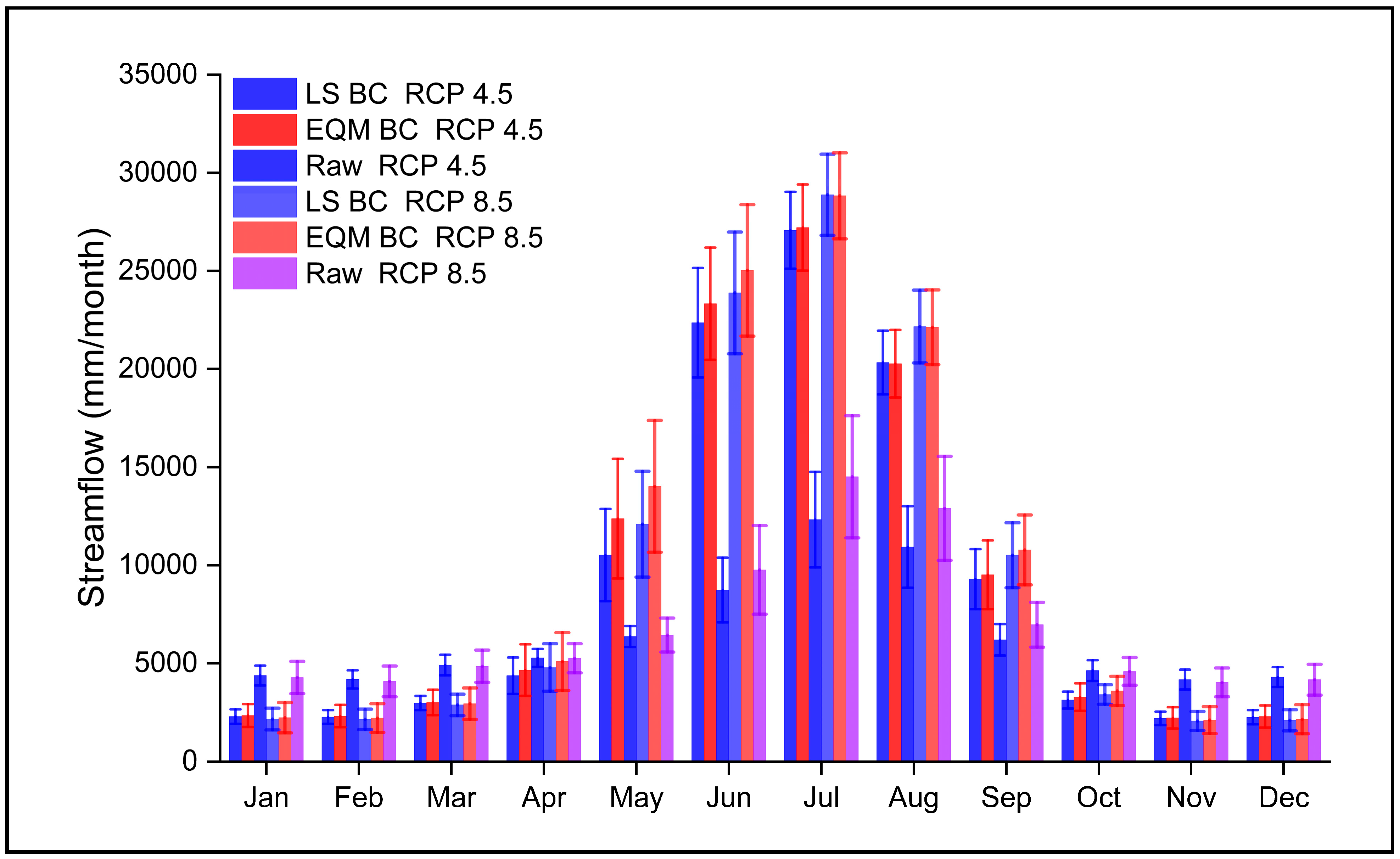
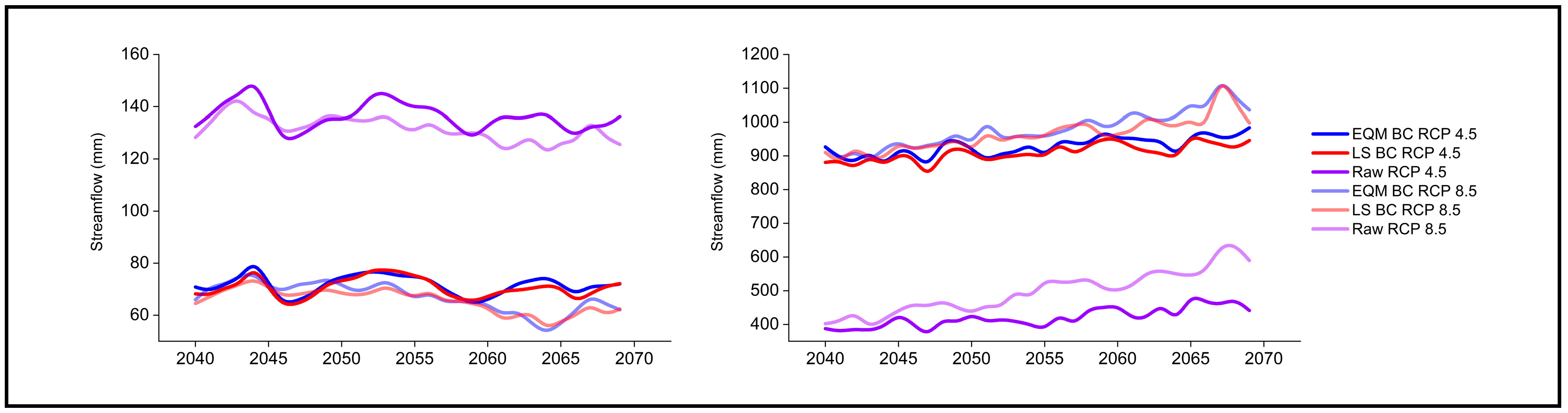
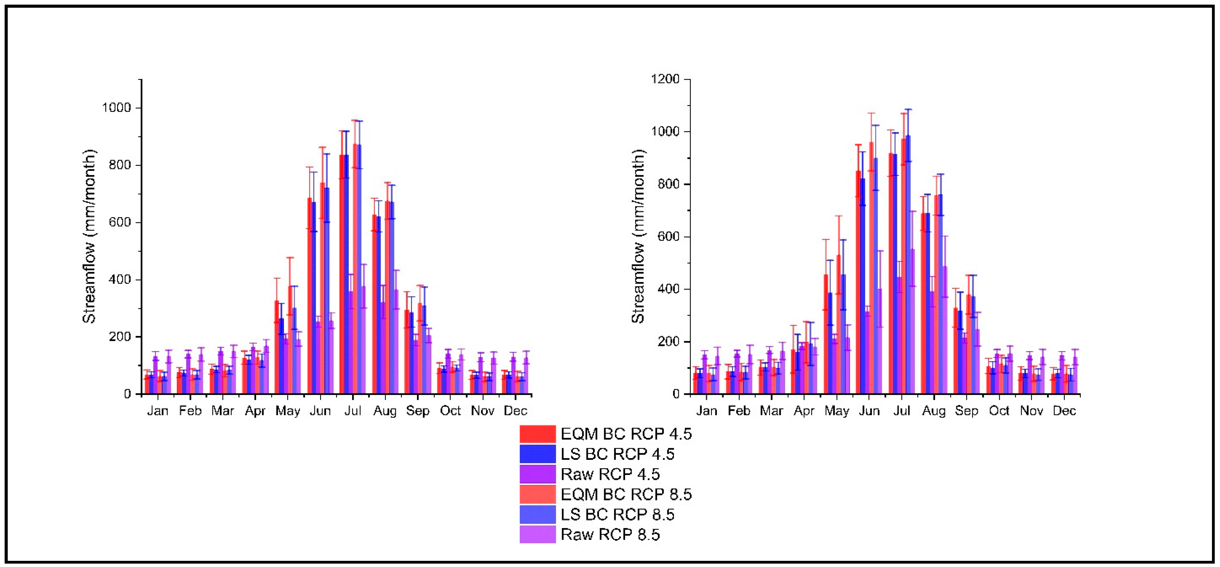
3.3. Impacts of Bias Correction on Projected Mid Future Hydrometeorological Conditions

Figure 5 shows the projected annual cycle for precipitation in the CRB, as provided by the raw and LS- and EQM-corrected NEX-GDDP models for the mid-future (2040–2069) under the RCP 4.5 and RCP 8.5 emission scenarios. As compared to raw NEX-GDDP, both LS and EQM data introduce modifications in the temporal pattern. In particular, as compared to the raw NEX-GDDP models, both bias correction methods lead to considerably lower precipitation in July and August and substantially higher precipitation in October, both for RCP 4.5 and RCP 8.5. Note that the LM and EQM methods yielded similar projections, which kept compatibility with the annual cycle drawn from the observations during the reference period (Figure 3).

Likewise, for the case of temperature (Figure 6), the LS and EQM methods were also shown to similarly modify the signal projected by raw NEX-GDDP models. Particularly, both approaches correct the cold values exhibited by the raw NEX-GDDP models, which are far from the observed regime throughout the year (Figure 3).

Finally, Figure 7 shows the results obtained when the calibrated hydrological model, HBV-light, was forced with the raw and LS- and EQM-corrected NEX-GDDP models to project mid-future streamflow in the CRB for the period 2040–2069, under the RCP 4.5 and RCP 8.5 emission scenarios. As for precipitation and temperature, the streamflow projected by raw NEX-GDDP did not seem realistic at all, when compared to the observed one (Figure 3). However, the LS- and EQM-corrected models were shown to produce similar, realistic future annual cycles for streamflow. In particular, as compared to raw NEX-GDDP models, the bias-corrected ones projected higher streamflow values during the wet season (June–August) and low streamflow values during the rest of the year, under both the RCP 4.5 and RCP 8.5 emission scenarios.

Figure 8 allows us to assess the impact of the LS and EQM bias correction methods on the 7-day minimum and maximum streamflow, and Figure 9 illustrates 10th and 90th percentile streamflow for mid-future period (2040–2069), under the RCP 4.5 and RCP 8.5 emission scenarios. The raw NEX-GDDP models were shown to provide higher values than LS- and EQM-corrected ones for 7-day minimum streamflow. On the contrary, the 7-day maximum streamflow simulated using raw NEX-GDDP models was projected to be lower than the one obtained using simulated with LS- and EQM-corrected NEX-GDDP models. Likewise, the 10th and 90th percentile streamflow, simulated with raw NEX-GDDP models, were also projected to be considerably lower in the wet period and higher for rest of the year, as compared to the values obtained with bias-corrected data, which seem much more realistic.

All these results warn on the direct use of global datasets, such as NEX-GDDP, for impact studies at local scales, especially in regions with complex terrain characteristics, such as CRB. In particular, the biases (with respect to gauge-based observations) exhibited by this dataset for precipitation and temperate can originate unrealistic future projections of different hydrological characteristics, from the mean to the extremes. Nevertheless, our findings emphasize the importance of bias correction techniques in coping with this issue, providing realistic future scenarios and contributing, therefore, to minimizing misadaptation.

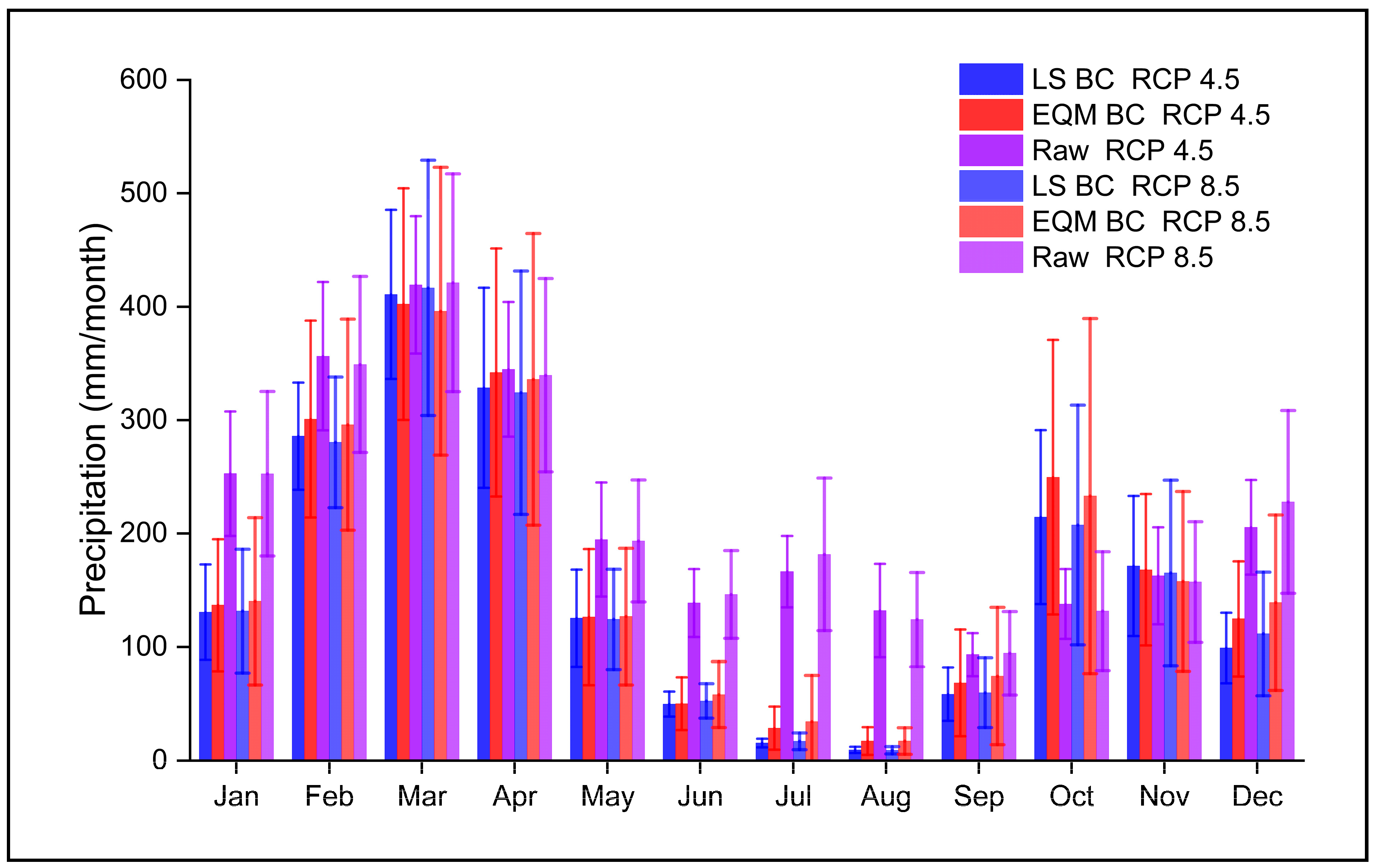
3.4. Impacts of Bias Correction on Projected Far Future Hydrometeorological Conditions

Figure 10 shows the projected annual cycle for precipitation in the CRB, as provided by raw and LS- and EQM-corrected NEX-GDDP models for the far future (2070–2099), under the RCP 4.5 and RCP 8.5 emission scenarios. Both LS and EQM data lead to modified temporal patterns, as compared to raw NEX-GDDP. Particularly, projected precipitation was significantly lower in July and August with both bias correction methods and was substantially higher in October and slightly higher in November. Likewise, the mid-future precipitation projections, i.e., the precipitation projected for the far future with both bias correction methods, depicts the compatibility with annual cycle of precipitation exhibited from observations during the reference period (Figure 3).

Moreover, for the case of temperature (Figure 11), both bias correction methods depicted modified signals, as compared to raw NEX-GDDP models, too. Similar to mid-future period, both bias correction methods corrected the cold values shown by the raw NEX-GDDP models, which were in noteworthy contrast to the observed regime throughout the year (Figure 3).

Figure 12 shows the results obtained when the calibrated hydrological model HBV-light was forced with raw and LS- and EQM-corrected NEX-GDDP models to project far future streamflow in the CRB for the period 2070–2099, under the RCP 4.5 and RCP 8.5 emission scenarios. It is clearly depicted that the streamflow projected by raw NEX-GDDP is not realistic, as compared to the observed streamflow (Figure 3). However, the LS- and EQM-corrected models are shown to produce similar, realistic far future annual cycles for streamflow. Particularly, higher streamflow values were projected with bias-corrected models during the wet season (June–August), as compared to raw NEX-GDDP models, and low streamflow values were projected during the rest of the year under both RCP 4.5 and RCP 8.5 emission scenarios. A relatively higher streamflow was projected with the raw NEX-GDDP models in the wet period under the RCP 8.5 emission scenario, as compared to the streamflow projected under the RCP 4.5 emission scenario; similarly, relatively higher streamflow was projected with LS- and EQM-corrected NEX-GDDP models in the wet period under the RCP 8.5 emission scenario, as compared to the RCP 4.5 emission scenario, depicting a noticeable impact of the extreme greenhouse gas emission scenario on the projected streamflow.

The impacts of LS- and EQM-bias correction methods on the 7-day minimum and maximum streamflow and 10th and 90th percentile streamflow for far future period (2070–2099) under the RCP 4.5 and RCP 8.5 emission scenarios are assessed with the help of Figure 13 and Figure 14, respectively. The raw NEX-GDDP models depict higher values for 7-day minimum streamflow than the LS- and EQM-corrected ones. On the other hand, the 7-day maximum streamflow, simulated using raw NEX-GDDP, was lower than the one obtained using the LS- and EQM-corrected NEX-GDDP models. In addition, the 10th and 90th percentile streamflow, simulated with the raw NEX-GDDP models, was also projected to be substantially lower in the wet period and higher for rest of the year, as compared to the values obtained with bias-corrected data, which seem much more realistic.

Like mid-future hydrometeorological projections, the results for the far future also negate the direct use of the high-resolution NEX-GDDP dataset for impact studies at local scales, particularly in regions with complex terrain characteristics, and accentuate the need of bias correction methods for removing the (region dependent) biases present in the raw NEX-GDDP models.

4. Conclusions

The Chitral River Basin (CRB) is one of the most important catchments within the Hindukush region of Pakistan. Its particularly complex terrain and large climate variability (which is linked to different monsoonal systems) play a key role in defining the hydrometeorological characteristics of the catchment and have a strong influence on water demand (including domestic and irrigation uses), hydropower generation, and food security, affecting millions of people living downstream. As such, it is crucial to develop adequate strategies that allow us to produce reliable long-term streamflow projections over the region. In this context, a key requirement is to have access to high-resolution, fine quality climatic information of temperature and precipitation, which are used as inputs for the hydrological models employed in impact studies [57,58,59]. In fact, climate models are generally selected based on the so-called “past performance approach”, i.e., on their ability to efficiently simulate the historical observed conditions [60,61]. Based on this premise, this study evaluates the adequacy of a widely used, high-resolution dataset, called NEX-GDDP, which comprises 21 state-of-the-art CMIP5 climate models, which have been statistically downscaled to a 0.25° × 0.25° regular grid for hydrological modeling in the CRB. Our results highlight that this dataset presents important biases for precipitation and temperature over the area of study, which, in turn, leads to unrealistic streamflow simulations, as revealed by comparison with the local observed data over a recent historical period. In order to cope with this issue, we also assessed the potential benefits of two different bias correction techniques, namely linear scaling (LS) and empirical quantile mapping (EQM), which are first shown to efficiently remove the mean errors found in the NEXGDDP models.

Then, the raw and LS- and EQM-corrected NEXGDDP data were used to feed the HBV-light hydrological model, which was used (after proper calibration/validation) to produce streamflow projections over the CRB for up to the end of 21st century, under two different emission scenarios, RCP 4.5 and RCP 8.5. The resulting projections strongly differed when the meteorological input variables (precipitation and temperature) were (not) bias-corrected, particularly in terms of the distribution of the annual cycle and extreme regimes.

In this study, both bias correction methods performed well in simulating reference streamflow for the CRB. As compared to the simplest bias correction strategy, LS, more sophisticated alternatives, such as EQM, do not seem to provide a clear advantage when used to correct the precipitation and temperature used as inputs for the hydrological modeling, leading to similar results, both in terms of the mean and extreme streamflow regimes. It should also be noted that the objective function for the hydrological model calibration could influence this result [41]. As demonstrated by [2], bias correction methods, which have performed well in simulating reference conditions, are expected to perform equally well in changing climatic conditions. In general, given that the BC approaches are designed to correct certain features of climate models, such as geographical, multivariate, temporal, and marginal aspects [55,62], it is clear that the bias-corrected climate change signal is accurately representative of the elements under consideration. Despite the stationarity issue, bias correction techniques are more likely to provide realistic estimates of the future climate than the raw model outputs, which had already exhibited a (relatively) poor performance over a recent historical reference period.

Therefore, this work warns on the use of raw NEXGDDP data for long-term hydrological modeling in complex terrain regions, where unrealistic future conditions could be obtained. Nevertheless, this important issue can be alleviated by using simple techniques, such as LS or EQM, to reduce the systematic errors present in forcing climate data. The findings of this study may extend beyond the NEX-GDDP dataset (used in this study) to other datasets that have low temporal or spatial resolution and may lead to misleading results in impact modeling. Finally, against the critique of [62], a multivariate-biased correction technique could be adopted to maintain the dependency structure between different variables used for hydrological simulations [55,63].

References

1. Teutschbein, C.; Wetterhall, F.; Seibert, J. Evaluation of different downscaling techniques for hydrological climate-change impact studies at the catchment scale. Clim. Dyn. 2011, 37, 2087–2105. [Google Scholar] [CrossRef]
2. Teutschbein, C.; Seibert, J. Bias correction of regional climate model simulations for hydrological climate-change impact studies: Review and evaluation of different methods. J. Hydrol. 2012, 456, 12–29. [Google Scholar] [CrossRef]
3. Siam, M.S.; Demory, M.-E.; Eltahir, E.A.B. Hydrological Cycles over the Congo and Upper Blue Nile Basins: Evaluation of General Circulation Model Simulations and Reanalysis Products. J. Clim. 2013, 26, 8881–8894. [Google Scholar] [CrossRef]
4. Hakala, K.; Addor, N.; Seibert, J. Hydrological Modeling to Evaluate Climate Model Simulations and Their Bias Correction. J. Hydrometeorol. 2018, 19, 1321–1337. [Google Scholar] [CrossRef]
5. Fowler, H.J.; Blenkinsop, S.; Tebaldi, C. Linking climate change modelling to impacts studies: Recent advances in downscaling techniques for hydrological modelling. Int. J. Clim. 2007, 27, 1547–1578. [Google Scholar] [CrossRef]
6. Grotch, S.L.; MacCracken, M.C. The use of general circulation models to predict regional climatic change. J. Climatology. 1991, 4, 286–303. [Google Scholar] [CrossRef]
7. IPCC. Climate Change 2007: The Physical Science Basis, Contribution of Working Group I to the Fourth Assessment Report of the Intergovernmental Panel on Climate Change; Cambridge University Press: Cambridge, UK; New York, NY, USA, 2007. [Google Scholar]
8. Salathé, E.P., Jr. Comparison of various precipitation downscaling methods for the simulation of streamflow in a rainshadow river basin. Int. J. Clim. 2003, 23, 887–901. [Google Scholar] [CrossRef] [Green Version]
9. Manzanas, R.; Gutiérrez, J.M.; Bhend, J.; Hemri, S.; Doblas-Reyes, F.J.; Torralba, V.; Penabad, E.; Brookshaw, A. Bias adjustment and ensemble recalibration methods for seasonal forecasting: A comprehensive intercomparison using the C3S dataset. Clim. Dyn. 2019, 53, 1287–1305. [Google Scholar] [CrossRef]
10. Mahrt, L. Variation of Surface Air Temperature in Complex Terrain. J. Appl. Meteorol. Clim. 2006, 45, 1481–1493. [Google Scholar] [CrossRef]
11. Minder, J.R.; Mote, P.W.; Lundquist, J.D. Surface temperature lapse rates over complex terrain: Lessons from the Cascade Mountains. J. Geophys. Res. Earth Surf. 2010, 115, D14122. [Google Scholar] [CrossRef]
12. Cannon, F.; Carvalho, L.M.V.; Jones, C.; Norris, J.; Bookhagen, B.; Kiladis, G.N. Effects of topographic smoothing on the simulation of winter precipitation in High Mountain Asia. J. Geophys. Res. Atmos. 2017, 122, 1456–1474. [Google Scholar] [CrossRef] [Green Version]
13. Bonekamp, P.N.J.; Collier, E.; Immerzeel, W.W. The impact of spatial resolution, landuse and spinup time on resolving spatial precipitation patterns in the Himalayas. J. Hydrometeorol. 2018, 19, 1565–1591. [Google Scholar] [CrossRef] [Green Version]
14. Ekström, M.; Grose, M.R.; Whetton, P.H. An appraisal of downscaling methods used in climate change research. WIREs Clim. Chang. 2015, 6, 301–319. [Google Scholar] [CrossRef]
15. Cannon, A.J. Negative ridge regression parameters for improving the covariance structure of multivariate linear downscaling models. Int. J. Clim. 2009, 29, 761–769. [Google Scholar] [CrossRef]
16. Charles, S.P.; Bates, B.C.; Smith, I.N.; Hughes, J.P. Statistical downscaling of daily precipitation from observed and modelled atmospheric fields. Hydrol. Process. 2004, 18, 1373–1394. [Google Scholar] [CrossRef]
17. Winkler, J.A.; Guentchev, G.S.; Perdinan; Tan, P.-N.; Zhong, S.; Liszewska, M.; Abraham, Z.; Niedźwiedź, T.; Ustrnul, Z. Climate Scenario Development and Applications for Local/Regional Climate Change Impact Assessments: An Overview for the Non-Climate Scientist: Part II: Considerations When Using Climate Change Scenarios. Geogr. Compass 2011, 5, 301–328. [Google Scholar] [CrossRef]
18. Thrasher, B.; Maurer, E.P.; McKellar, C.; Duffy, P.B. Technical Note: Bias correcting climate model simulated daily temperature extremes with quantile mapping. Hydrol. Earth Syst. Sci. 2012, 16, 3309–3314. [Google Scholar] [CrossRef] [Green Version]
19. Wood, A.W.; Maurer, E.P.; Kumar, A.; Lettenmaier, D.P. Long-range experimental hydrologic forecasting for the eastern United States. J. Geophys. Res. Atmo. 2002, 107, 4429. [Google Scholar] [CrossRef]
20. Wood, A.; Leung, L.R.; Sridhar, V.; Lettenmaier, D.P. Hydrologic Implications of Dynamical and Statistical Approaches to Downscaling Climate Model Outputs. Clim. Chang. 2004, 15, 189–216. [Google Scholar] [CrossRef]
21. Maurer, E.P.; Hidalgo, H.G. Utility of daily vs. monthly large-scale climate data: An intercomparison of two statistical downscaling methods. Hydrol. Earth Syst. Sci. 2008, 12, 551–563. [Google Scholar] [CrossRef]
22. Xu, R.; Chen, Y.; Chen, Z. Future Changes of Precipitation over the Han River Basin Using NEX-GDDP Dataset and the SVR_QM Method. Atmosphere 2019, 10, 688. [Google Scholar] [CrossRef] [Green Version]
23. Guo, X.; Yang, Y.; Li, Z.; You, L.; Zeng, C.; Cao, J.; Hong, Y. Drought Trend Analysis Based on the Standardized Precipitation–Evapotranspiration Index Using NASA’s Earth Exchange Global Daily Downscaled Projections, High Spatial Resolution Coupled Model Intercomparison Project Phase 5 Projections, and Assessment of Potential Impacts on China’s Crop Yield in the 21st Century. Water 2019, 11, 2455. [Google Scholar] [CrossRef] [Green Version]
24. Raghavan, S.V.; Hur, J.; Liong, S.-Y. Evaluations of NASA NEX-GDDP data over Southeast Asia: Present and future climates. Clim. Chang. 2018, 148, 503–518. [Google Scholar] [CrossRef]
25. Sahany, S.; Mishra, S.K.; Salunke, P. Historical simulations and climate change projections over India by NCAR CCSM4: CMIP5 vs. NEX-GDDP. Theor. Appl. Climatol. 2019, 135, 1423–1433. [Google Scholar] [CrossRef]
26. Jain, S.; Salunke, P.; Mishra, S.K.; Sahany, S.; Choudhary, N. Advantage of NEX-GDDP over CMIP5 and CORDEX Data: Indian Summer Monsoon. Atmos. Res. 2019, 228, 152–160. [Google Scholar] [CrossRef]
27. Tebaldi, C.; Knutti, R. The use of the multi-model ensemble in probabilistic climate projections. PPhilos. Trans. R. Soc. A Math. Phys. Eng. Sci. 2007, 365, 2053–2075. [Google Scholar] [CrossRef]
28. Charles, S.P.; Bates, B.C.; Whetton, P.H.; Hughes, J.P. Validation of downscaling models for changed climate conditions: Case study of southwestern Australia. Clim. Res. 1999, 12, 1–14. [Google Scholar] [CrossRef] [Green Version]
29. Jun, M.; Knutti, R.; Nychka, D.W. Spatial Analysis to Quantify Numerical Model Bias and Dependence. J. Am. Stat. Assoc. 2008, 103, 934–947. [Google Scholar] [CrossRef]
30. Knutti, R. Should we believe model predictions of future climate change? Philos. Trans. R. Soc. London. Ser. A Math. Phys. Eng. Sci. 2008, 366, 4647–4664. [Google Scholar] [CrossRef]
31. Li, C.; Sinha, E.; Horton, D.E.; Diffenbaugh, N.S.; Michalak, A.M. Joint bias correction of temperature and precipitation in climate model simulations. J. Geophys. Res. Atmos. 2014, 119, 13153–13162. [Google Scholar] [CrossRef]
32. Sharma, D.; Das Gupta, A.; Babel, M.S. Spatial disaggregation of bias-corrected GCM precipitation for improved hydrologic simulation: Ping River Basin, Thailand. Hydrol. Earth Syst. Sci. 2007, 11, 1373–1390. [Google Scholar] [CrossRef] [Green Version]
33. Hansen, J.; Challinor, A.; Ines, A.; Wheeler, T.; Moron, V. Translating climate forecasts into agricultural terms: Advances and challenges. Clim. Res. 2006, 33, 27–41. [Google Scholar] [CrossRef]
34. Räisänen, J.; Räty, O. Projections of daily mean temperature variability in the future: Cross-validation tests with ENSEMBLES regional climate simulations. Clim. Dyn. 2012, 41, 1553–1568. [Google Scholar] [CrossRef]
35. Usman, M.; Pan, X.; Penna, D.; Ahmad, B. Hydrologic alteration and potential ecosystemic implications under a changing climate in the Chitral River, Hindukush region, Pakistan. J. Water Clim. Chang. 2021, 12, 1471–1486. [Google Scholar] [CrossRef]
36. Xu, L.; Wang, A. Application of the Bias Correction and Spatial Downscaling Algorithm on the Temperature Extremes From CMIP5 Multimodel Ensembles in China. Earth Space Sci. 2019, 6, 2508–2524. [Google Scholar] [CrossRef] [Green Version]
37. Bergström, S. Development and Application of a Conceptual Runoff Model for Scandinavian Catchments. Norrköping 1976, 134. [Google Scholar]
38. Lindström, G.; Johansson, B.; Persson, M.; Gardelin, M.; Bergström, S. Development and test of the distributed HBV-96 hydrological model. J. Hydrol. 1997, 201, 272–288. [Google Scholar] [CrossRef]
39. Seibert, J.; Vis, M.J.P. Teaching hydrological modeling with a user-friendly catchment-runoff-model software package. Hydrol. Earth. Sys. Sci. 2012, 16, 3315–3325. [Google Scholar] [CrossRef] [Green Version]
40. Seibert, J. Multi-criteria calibration of a conceptual runoff model using a genetic algorithm. Hydrol. Earth Syst. Sci. 2000, 4, 215–224. [Google Scholar] [CrossRef] [Green Version]
41. Adeyeri, O.; Laux, P.; Arnault, J.; Lawin, A.; Kunstmann, H. Conceptual hydrological model calibration using multi-objective optimization techniques over the transboundary Komadugu-Yobe basin, Lake Chad Area, West Africa. J. Hydrol. Reg. Stud. 2020, 27, 100655. [Google Scholar] [CrossRef]
42. Seibert, J. HBV Light Version 2. In User’s Manual; Department of Physical Geography and Quaternary Geology, Stockholm University: Stockholm, Sweden, 2005. [Google Scholar]
43. Usman, M.; Ndehedehe, C.E.; Farah, H.; Manzanas, R. Impacts of climate change on the streamflow of a large river basin in the Australian tropics using optimally selected climate model outputs. J. Clean. Prod. 2021, 315, 128091. [Google Scholar] [CrossRef]
44. Usman, M.; Ndehedehe, C.E.; Farah, H.; Ahmad, B.; Wong, Y.; Adeyeri, O.E. Application of a Conceptual Hydrological Model for Streamflow Prediction Using Multi-Source Precipitation Products in a Semi-Arid River Basin. Water 2022, 14, 1260. [Google Scholar] [CrossRef]
45. Teutschbein, C.; Seibert, J. Regional Climate Models for Hydrological Impact Studies at the Catchment Scale: A Review of Recent Modeling Strategies. Geogr. Compass 2010, 4, 834–860. [Google Scholar] [CrossRef] [Green Version]
46. Manzanas, R.; Fiwa, L.; Vanya, C.; Kanamaru, H.; Gutiérrez, J.M. Statistical downscaling or bias adjustment? A case study involving implausible climate change projections of precipitation in Malawi. Clim. Chang. 2020, 162, 1437–1453. [Google Scholar] [CrossRef]
47. Lachenbruch, P.A.; Mickey, M.R. Estimation of Error Rates in Discriminant Analysis. Technometrics 1968, 10, 1–11. [Google Scholar] [CrossRef]
48. Ines, A.V.M.; Hansen, J.W. Bias correction of daily GCM rainfall for crop simulation studies. Agri. Forest. Meteorol. 2006, 138, 44–53. [Google Scholar] [CrossRef] [Green Version]
49. Shrestha, S.; Shrestha, M.; Babel, M.S. Assessment of climate change impact on water diversion strategies of Melamchi Water Supply Project in Nepal. Theor. Appl. Climatol. 2015, 128, 311–323. [Google Scholar] [CrossRef]
50. Lenderink, G.; Buishand, A.; Van Deursen, W. Estimates of future discharges of the river Rhine using two scenario methodologies: Direct versus delta approach. Hydrol. Earth Syst. Sci. 2007, 11, 1145–1159. [Google Scholar] [CrossRef]
51. Fang, G.H.; Yang, J.; Chen, Y.N.; Zammit, C. Comparing bias correction methods in downscaling meteorological variables for a hydrologic impact study in an arid area in China. Hydrol. Earth Syst. Sci. 2015, 19, 2547–2559. [Google Scholar] [CrossRef] [Green Version]
52. Block, P.J.; Souza Filho, F.A.; Sun, L.; Kwon, H.H. A Stream-flow Forecasting Framework using Multiple Climate and Hydrological Models. J. Am. Water. Resour. Assoc. 2009, 45, 828–843. [Google Scholar] [CrossRef]
53. Déqué, M.; Rowell, D.P.; Lüthi, D.; Giorgi, F.; Christensen, J.H.; Rockel, B.; Jacob, D.; Kjellström, E.; de Castro, M.; Hurk, B.V.D. An intercomparison of regional climate simulations for Europe: Assessing uncertainties in model projections. Clim. Chang. 2007, 81, 53–70. [Google Scholar] [CrossRef]
54. Mendez, M.; Maathuis, B.; Hein-Griggs, D.; Alvarado-Gamboa, L.-F. Performance Evaluation of Bias Correction Methods for Climate Change Monthly Precipitation Projections over Costa Rica. Water 2020, 12, 482. [Google Scholar] [CrossRef] [Green Version]
55. Adeyeri, O.E.; Laux, P.; Lawin, A.E.; Oyekan, K.S.A. Multiple bias-correction of dynamically downscaled CMIP5 climate models temperature projection: A case study of the transboundary Komadugu-Yobe river basin, Lake Chad region, West Africa. SN Appl. Sci. 2020, 2, 1221. [Google Scholar] [CrossRef]
56. Manzanas, R.; Lucero, A.; Weisheimer, A.; Gutiérrez, J.M. Can bias correction and statistical downscaling methods improve the skill of seasonal precipitation forecasts? Clim. Dyn. 2018, 50, 1161–1176. [Google Scholar] [CrossRef] [Green Version]
57. Böhner, J.; Lehmkuhl, F. Environmental change modelling for Central and High Asia: Pleistocene, present and future scenarios. Boreas 2008, 34, 220–231. [Google Scholar] [CrossRef]
58. Karmacharya, J.; Jones, R.; Moufouma-Okia, W.; New, M. Evaluation of the added value of a high-resolution regional climate model simulation of the South Asian summer monsoon climatology. Int. J. Clim. 2016, 37, 3630–3643. [Google Scholar] [CrossRef]
59. Gerlitz, L.; Bechtel, B.; Böhner, J.; Bobrowski, M.; Bürzle, B.; Müller, M.; Scholten, T.; Schickhoff, U.; Schwab, N.; Weidinger, J. Analytic Comparison of Temperature Lapse Rates and Precipitation Gradients in a Himalayan Treeline Environment: Implications for Statistical Downscaling. In Climate Change, Glacier Response, and Vegetation Dynamics in the Himalaya; Springer: Berlin/Heidelberg, Germany, 2016; pp. 49–64. [Google Scholar] [CrossRef]
60. Pierce, D.W.; Barnett, T.P.; Santer, B.D.; Gleckler, P.J. Selecting global climate models for regional climate change studies. Proc. Natl. Acad. Sci. USA 2009, 106, 8441–8446. [Google Scholar] [CrossRef] [Green Version]
61. Biemans, H.; Speelman, L.; Ludwig, F.; Moors, E.; Wiltshire, A.; Kumar, P.; Gerten, D.; Kabat, P. Future water resources for food production in five South Asian river basins and potential for adaptation—A modeling study. Sci. Total Environ. 2013, 468, S117–S131. [Google Scholar] [CrossRef]
62. Maraun, D. Nonstationarities of regional climate model biases in European seasonal mean temperature and precipitation sums. Geophys. Res. Lett. 2012, 39, 6. [Google Scholar] [CrossRef] [Green Version]
63. Dieng, D.; Cannon, A.J.; Laux, P.; Hald, C.; Adeyeri, O.; Rahimi, J.; Srivastava, A.K.; Mbaye, M.L.; Kunstmann, H. Multivariate Bias-Correction of High-Resolution Regional Climate Change Simulations for West Africa: Performance and Climate Change Implications. J. Geophys. Res. Atmos. 2022, 127, e2021JD034836. [Google Scholar] [CrossRef]
Figure 1. Location and physiographic map of the Chitral River Basin (basemap reference; Esri, DeLorme, HERE, MapmyIndia).
Hydrology 09 00188 g001
Figure 2. Top left: daily observed (black) and HBV-light simulated (grey) streamflow during the calibration period (1995–2007). Top right: as top left, but for the validation period (2008–2012). Bottom panels: measure of fit (including the R2 coefficient) between daily observed and HBV-light simulated streamflow during the calibration (left) and validation (right) periods.
Hydrology 09 00188 g002
Figure 3. Left: mean monthly precipitation (left), temperature (center), and streamflow (right), as provided by observed station data (Obs) and the ensemble mean of the 21 NEX-GDDP models when they were LS-corrected (LS BC), EQM-corrected (EQM BC), and their raw outputs (Raw) were considered for the reference period (1995–2005). The error bars represent the standard deviation across the 21 models.
Hydrology 09 00188 g003
Figure 4. Top left: inter-annual time-series of 7-day minimum streamflow, as provided by observed station data (Obs) and the ensemble mean of the 21 NEXGDDP models when they were LS-corrected (LS BC), EQM-corrected (EQM BC), and their raw outputs (Raw) were considered for the reference period (1995–2005). Top right: as top left, but for 7-day maximum streamflow. Bottom panels: as Figure 3, but for 10th percentile (left) and 90th percentile (right) streamflow throughout 1995–2005.
Hydrology 09 00188 g004
Figure 5. Mean monthly precipitation, as provided by the ensemble mean of the 21 NEX-GDDP models when they are LS-corrected (LS BC), EQM-corrected (EQM BC), and when their raw outputs (Raw) are considered. The error bars represent the standard deviation across the 21 models for the period 2040–2069.
Hydrology 09 00188 g005
Figure 6. As Figure 5, but for mean monthly temperature.
Hydrology 09 00188 g006
Figure 7. As Figure 5, but for mean monthly streamflow.
Hydrology 09 00188 g007
Figure 8. Left panel: inter-annual time-series of 7-day minimum streamflow, as provided by the ensemble mean of the 21 NEXGDDP models when they are LS-corrected (LS BC), EQM-corrected (EQM BC), and when their raw outputs (Raw) are considered for the period (2040–2069). Right panel: as left panel, but for 7-day maximum streamflow.
Hydrology 09 00188 g008
Figure 9. As Figure 8, but for 10th percentile (left) and 90th percentile (right) streamflow over the period 2040–2069.
Hydrology 09 00188 g009
Figure 10. As Figure 5, but for the period 2070–2099.
Hydrology 09 00188 g010
Figure 11. As Figure 6, but for the period 2070–2099.
Hydrology 09 00188 g011
Figure 12. As Figure 7, but for the period 2070–2099.
Hydrology 09 00188 g012
Figure 13. As Figure 8, but for the period 2070–2099.
Hydrology 09 00188 g013
Figure 14. As Figure 9, but for the period 2070–2099.
Hydrology 09 00188 g014
Publisher’s Note: MDPI stays neutral with regard to jurisdictional claims in published maps and institutional affiliations.