1. Introduction
Extreme events are the most impacting phenomena on society and infrastructure worldwide, and they present the greatest challenges for managers and technicians to design and implement mitigation measures. Information on the impact and trends of these events can improve the estimates of future events and can thus be used to support political decisionmaking and flood management and to control system design [
1].
The importance of hydro-climate estimates is demonstrated in the large number of scientific papers that have been published recently aimed at the improvement of probabilistic estimates [
2,
3,
4,
5]. Comparative studies of parameter estimation methods have been widely used to analyse hydro-climate extremes. The need to improve these estimates is supported by the application of new mathematical tools to describe natural phenomena such as artificial intelligence [
6].
Table 1 presents three more studies about the subject. In the study of Ribeiro Junior et al. [
7], normal distribution is applied to the precipitation series by the use of nonparametric methods, which determine the non-homogeneity in rainfall series and subsidize rainfall–runoff modelling of large basins.
The homogeneity of natural climate time series has also gained prominence regarding identifying decadal variations in rainfall series [
1,
8,
9,
10] or heat flows from the Antarctic seas associated with the El Niño Southern Oscillation [
11], which influences global climate.
The fluctuation in precipitation regimes is a complicated phenomenon that can cause significant impacts on environmental and socioeconomic components (e.g., disrupting water supply and demand, impacting vegetation, and causing floods or droughts) [
8,
9,
10,
11,
12]. Identifying the pattern of decadal precipitation fluctuations is critical because it can help us manage water supply and mitigate natural disasters such as floods and droughts, which often occur around the world [
13]. As precipitation estimates are notoriously uncertain, particularly for extreme local events, a probabilistic method is generally used to simulate possible scenarios. Despite the calculation method, rainfall frequency analyses are used for the estimation of design rainfalls [
14], which are totally related to the infrastructure design in urban areas. Flash floods areurban hazards and are associated with extreme short-term rainfalls in daily or hourly scales [
15,
16,
17]. They occur due to the low capacity of the catchments to accumulate runoff discharge [
18].
Table 1.
Comparative studies assessing different parameter estimation methods for the analyses of hydro-climate extremes.
Table 1.
Comparative studies assessing different parameter estimation methods for the analyses of hydro-climate extremes.
| Reference | Variable | Location (Number of Sites) | Sample Size (Years) | Distributions
or Other Methodologies | Methods | Evaluation Criteria |
|---|
| [19] | floods | Pakistan (18) | not available | GLO, GEV, GPA | LH-moments, Goodness-of-Fit | Anderson Darling, Kolmogorov–Smirnov, Cramér–Von Mises, t-test |
| [20] | Precipitation | Crete
(Greece)
(54) | 41 | GAM, GEV, LGN, WBL, P-II | KDE, BGK | KCDE-ITS, CDF, ERA5—Copernicus Climate Change Service |
| [7] | Precipitation and average river flow | Brazil (22) | 51 | ND | MGB-IPH, ETA model/A1B/IPCC | Mann–Kendall, Pettitt, Run, Spearman |
One of the major issues of our day is predicting extreme hydrological occurrences in the long and medium terms under non-stationary settings [
21]. Runoff discharge and temporal rainfall are among the hydrological phenomena that can be considered as stochastic processes with random variables within a given probability distribution, for which time series demonstrations are widely used [
21,
22]. As per Koutsoyiannis and Montanari [
23], the concept of stationarity is used to describe a probability density function which may not be changed in time. Thus, the calculation of distribution quantiles (i.e., division of a probability distribution into equal probability areas) associated with a specific non-exceedance probability is one of the challenges of extreme event frequency analysis. They are frequently calculated when a probabilistic model is fitted to observable data [
21].
According to Totaro et al. [
21], nonparametric measures of trends have been used for the detection of non-stationary conditions in extreme events, including statistical tests such as Mann–Kendall [
24] and Spearman [
25] as well as the Pettitt’s [
26] tests for change point detection. They are all founded on a specific null hypothesis to achieve a certain significance level. However, despite its nonparametric structure, Mann–Kendall test effectiveness depends on the kind and parameterization of the parent distribution [
27].
Due to being distribution-free, not requiring extensive knowledge about the parent distribution and being less sensitive to the presence of outliers, these non-parametric tests are frequently favoured over parametric tests for the frequency analysis of extreme events [
28,
29].
2. Materials and Methods
In the study of the variation of extreme flows, we used the maximum annual flows from the hydrological history of daily flows. For the study, we selected the gauging station 4C-001 in Pardo River, which is part of the Mogi-Guaçu River catchment, in the City of Ribeirao Preto, State of São Paulo, Brazil.
This hydrological series was selected because it has good quantitative and qualitative historical data (i.e., updated extent of historical series, no incomplete years of observations, and only a few gaps for filling or with non-consistent information). The location, analysed period, and watershed area are shown in
Table 2.
Daily flow rate updates are the responsibility of the Hydraulic Technology Centre (CTH) of the University of Sao Paulo (USP), operated by the Department of Water and Electric Energy of the State of Sao Paulo (DAEE).
Selecting the “ideal size” of a hydrological series is challenging, especially when the data are scarce, but the main criterion considered for this study was to choose a long and good-quality data series. If it is not long enough, it becomes more complex to acknowledge the hydrological behaviour of the local extreme events. The fluctuation evaluations show the distinguished climate features of extreme events. This procedure is essential in estimating design rainfall and water availability, among other input parameters used by hydrologists to produce outcomes and to support efficient infrastructure design and urban planning.
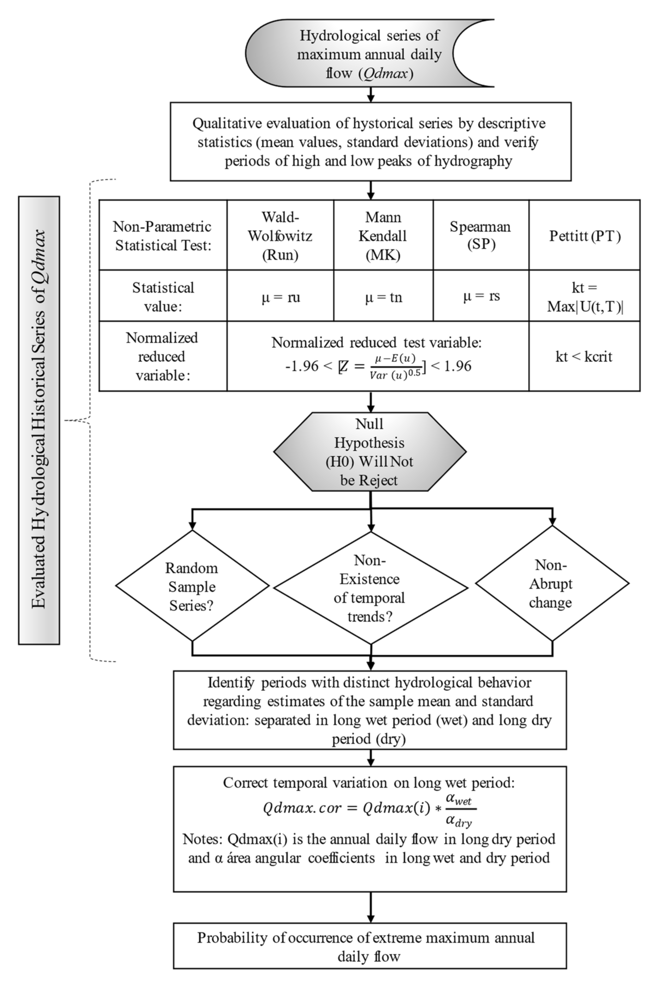
Initially, the study of the hydrological series comprised qualitative evaluation using descriptive statistics (averages and standard deviations) and by the analysis of the periods of high and low peaks of the hydrograph. Then, we evaluated if the hydrological historical series was representative, random and without statistically significant trends. To assess whether the variations in the hydrological historical series occurred randomly, the non-parametric Wald–Wolfowitz statistical test was applied, known as the run test (oscillations). If the run test is being tested for randomness, then it is understood that the data should come into the dataset as an ordered sample, increasing in magnitude.
According to Ribeiro Junior [
30], the run test counts the number of oscillations of the values above the reference measure (median) (i.e., positive, and negative values, respectively), in a naturally ordered data series. This number of oscillations is called “Run”, and the accounting of each oscillation is computed when there is a change between the positive and negative oscillations, or viceversa. For instance, when a value above the median (positive oscillation) is preceded by another, also oscillating in the positive range, it is not considered a variation of the oscillation and therefore is not counted as a run. However, if the preceding value is below the median (negative oscillation) it shows the occurrence of a variation and therefore is considered a run. If the number of values, either above the median (positive variations,
N1) or below it (negative variations,
N2) is greater than 20, the sample is considered large, and the run value sample distribution approaches the normal distribution. The expected value (
E) and variance (
Var) are calculated by Equations (1) and (2), respectively.
in which
ru is the number of oscillations or runs as well as the statistical value of the test,
N1 is the number of observations above the median (positive variations), and
N2 is the number of observations below the median (negative variations).
Once the test distribution is approaching the normalization, the reduced variable value of the test is calculated by Equation (3). Adopting a significance level of 5%, the null hypothesis (
H0 for a random sample series) will not be rejected if the calculated value (
Z, reduced variable) is between [−1.96; +1.96].
in which
Z is the value of the reduced variable to the standard normal distribution and is derived by the statistical test, and
u is the statistical value of the hypothesis test.
To assess whether there was a temporal trend in the historical hydrological series of the maximum annual daily flows (Qdmax), we combined the non-parametric statistical tests of Spearman (SP), Mann–Kendall (MK) and Pettitt (PT).
According to Pellegrino [
31], to estimate the sequential test of MK, the
tn statistic is initially calculated by Equation (4), considering the time series of the
Yi variable (maximum annual daily flows,
Qdmax) of
N observations (years). This equation consists of determining the sum of the number of terms (
mi) in the series, relative to the value
Yi, whose preceding terms (
j <
i) account for the number of values
Yj < Yi.
in which
tn is the value of the MK test, and
mi is the number of preceding observations that satisfy the condition
Yj < Yi, where
j < i.We used Equation (3) for the significance test of
tn, represented as
Z(
tn), which is the two-sided test for normal distribution. The expected value of the test and the variance were calculated by Equations (5) and (6), respectively.
in which
E(
tn) is the expected value of the MK test with
Var(
tn) being the variance of the MK test.
The calculated value of Z(tn) is compared to the reduced variable of the normal distribution (z) extracted from the statistical tables and associated with the significance levels of: (i) 10% (significant), where z = 1.64, and (ii) 5% (highly significant), where z = 1.96.
The test hypotheses are: (i) H0, if there is no time trend, and (ii) Ha if there is a time trend. The purpose of the test is to verify whether the null hypothesis can be accepted or rejected, and thus, the module of the ZMK value must not exceed the tabulated one.
To confirm the non-existence of a monotonous temporal trend for the hydrological series, the Spearman’s non-parametric test was simultaneously employed. This test estimates the correlation coefficient between the series and the time index [
32]. The value of the test statistic (
rs) is calculated by Equation (7), in which the order of the increasing position of the values of the series (
mi) is subtracted by the temporal position (time index,
Ti).
where
mi is the position of the observed event, regarding the increasing order of the values of the hydrological sample series,
Ti is the sequential time composition of the event, and
N is the number of observations of the sample series (number of observed years).
For large samples,
rs approaches the reduced normal distribution and is calculated by Equation (3). The expected value is null, and the test variance is calculated by Equation (8). For a significance level of 5%, if the calculated
Z-value is between [−1.96; +1.96], the null hypothesis is not rejected, and the series is considered stationary. The variance of the SP test is derived from Equation (8).
The point of abrupt change or beginning of the trend was determined by the non-parametric Pettitt’s test. This test verifies that two samples of the same series belong to the same population: (i) Xi, …, Xt−1 and (ii) Xt, …, Xn.
The statistics
U(
t,
N) of this test are calculated by Equation (9), which is the total number of times that the observation of the first sample is larger than the members of the second. The variable
U(
t,
N) is calculated sequentially for all values of the hydrological series, as presented by Equation (9).
where,
in which
U(
i,
N) is the Pettitt’s statistic value for the observation
yi,
U(
i−
1,
N) is the Pettitt’s statistic value for the previous observation
yi−1, and
yi is the value of the observation in the
i order of the historical series. The variable
U(
t,
N) is calculated sequentially for all values of the hydrological series, in which
k(
t) is the test value being the absolute maximum, as presented by Equation (10).
According to Back [
33], the test significance is estimated by Equation (11):
in which
p is the test significance for the desired significance level (α
o).
Based on Equation (11) and isolating the value of
k(
t), we obtain Equation (12), associating the probability of significance level of
αo = 5%, and we calculate the critical value of the Pettitt’s statistic, which is
kcrit.
To prove that there was some abrupt change in the hydrological series and that it is not stationary, the module of the
k(
t) statistic should be greater than the
kcrit [
33].
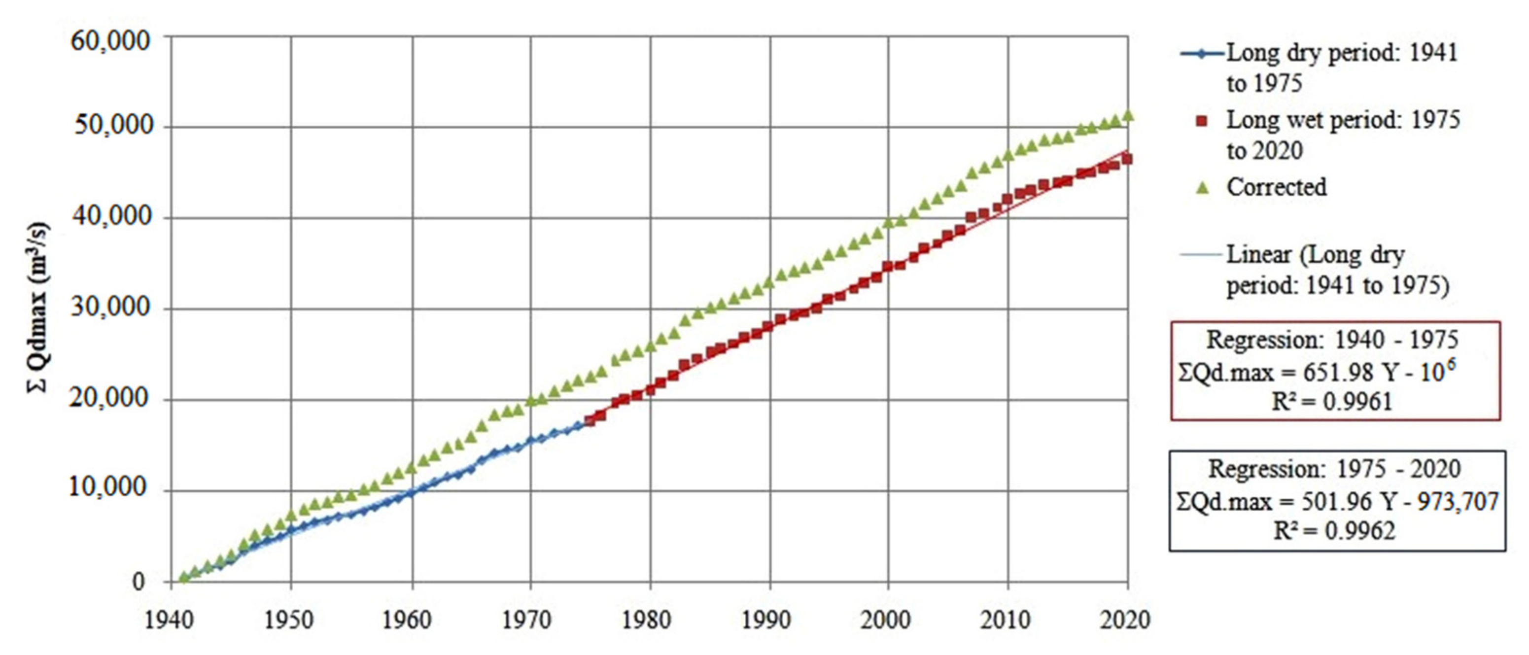
Once the stationary nature of the river flow series has been confirmed, we proceed to identify the periods with distinct hydrological behaviour in relation to the estimates of the sample mean and standard deviation. These estimates were prepared for two periods: (i) the beginning of the hydrological series from 1941 to 1975, which corresponds to the long dry period, and (ii) between 1975 and 2020, which is the long wet period. The first interval represents the series featured by the driest period, which comprises the lowest observed maximum flows. In the following period, there was a change in both sample mean and standard deviation.
Once a periodic variability was identified in the hydrological series of maximum annual daily flows, these values were corrected, eliminating the temporal variation. For that, we used the methodology adapted from Detzel et al. [
34] in the current study.
On the accumulative curve of the hydrological variable, time is represented on the horizontal axis, and the sum of the maximum annual flow is on the vertical axis. According to Detzel et al. [
34], this method is based on the fact that by plotting the graph of the accumulative curve of the hydrological variable, it is possible to adjust the linear regression of continuous trend over the time horizon. In the study, a non-stationary pattern was identified by the change in curve slope, where it was possible to divide it into two linear regressions.
The correction for non-stationarity was carried out by adjusting the angular coefficients of the two fitted straight lines:
The historical series was divided into two periods, and the limit of these new series was defined by the year of the maximum value of the statistic indicated by the PT test.
The angular coefficients were estimated for both periods of the divided series.
To linearize the trend, the Qdmax of the oldest period (i.e., the beginning of the series related to the rupture year) was multiplied by the relation of the linear coefficients of the recent period over the previous one.
The result of the correction is a random, stationary series in which the previous period (beginning of the series related to the year of rupture) is increased by the angular coefficient of the recent period, in which the observed values remain. The corrected series eliminates the long dry period, maximizing the estimates of design flows for hydraulic works.
To estimate the probability of occurrence of extreme maximum events, we used the Fisher–Tippet Type I distribution, commonly referred to as Gumbel distribution. The form of this probability function (
FD) is shown in Equation (13).
where
FD (
Yi) is the cumulative likelihood function for the random variable.
The parameters α and β were estimated by the maximum likelihood method, as suggested by Beijo [
35] and Bautista [
36] and as shown in Equations (14) and (15), respectively.
in which
Ym is the sample mean of the random variable,
is the scale parameter, and
is the position parameter.
Finally, we used the Kolmogorov–Smirnov test as described in Naghettini and Pinto [
32] to assess whether the data fitted the theoretical probability distribution.
Figure 1 presents the flowchart of the methodology developed in this study.
For the estimation of the non-parametric statistical tests and adjustment of the Gumbel probability distribution parameters, scripts of these subroutines were developed in VBA (Visual Basic Application) programming language, implemented in the calculation platform of the Microsoft EXCEL®.
3. Results and Discussion
The application of non-parametric statistical tests for the annual maximum daily flow series (
Qdmax) is presented in
Table 3, where we summarized the estimates of variables for the tests of randomness (run) and trend (SP, MK and PT).
Analysing the significance level in
Table 2, when
H0 is 10%, it does not reject
H0 for
αo = 10%. However, if
H0 is 5%, it does not reject
H0 for
αo = 5%, and if it is
Ha, it rejects
H0 regarding the trend.
For the significance level of 10%, the studied hydrological series was considered random (the statistic test ZRun was—1.80). For the MK trend test, the calculated value of the ZMK statistic was 0.98, which indicated non-rejection of the null hypothesis (i.e., the non-existence of a trend at a 5% significance level).
The module of the highest estimated value of the Pettitt test variable (Kt) was 459, which occurred for the year 1975. This result is lower than the critical limit (kcrit = 576), and therefore, the oscillations of the annual maximum daily water levels were stationary without the occurrence of any abrupt change in the series.
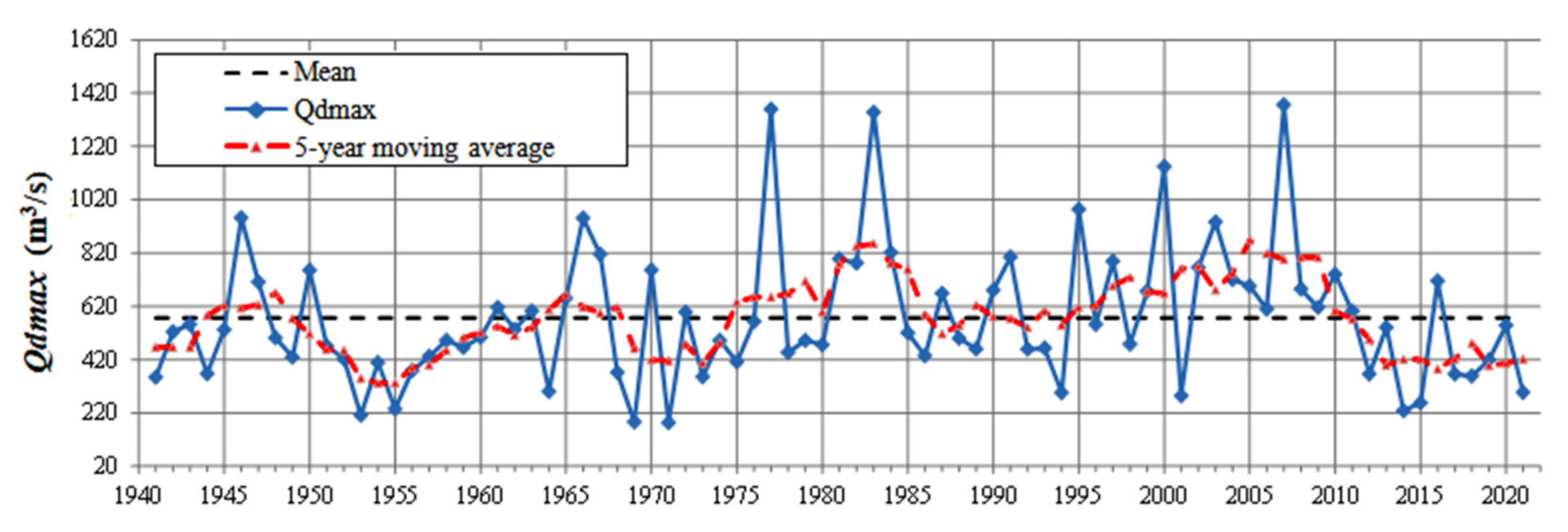
We have elaborated the graph of the 4C-001 hydrological series to analyse the historical behaviour of the annual maximum daily water levels (
Qdmax), as shown in
Figure 2. The black and red dashed lines represent the multi-annual sample mean and the 5-year moving average, respectively.
Throughout the centred five-year moving average of the maximum annual daily flow rate, three distinct periods for Qdmax in the Pardo River can be highlighted:
From 1940 to 1975: the initial time interval of the historical series whose Qdmax values were either close to the sample mean, or lower. This period showed a descending behaviour of the hydrological variable.
From 1975 to 2010: in this period of the hydrological series, the studied variable showed a strongly increasing behaviour, where the highest values of maximum flow of 1376.6 occurred in 2007, followed by 1348.8 in 1983. These higher magnitudes of Qdmax had not occurred in the series until previous years.
From 2010: in the current period of the series, maximum flow values were either close to the sample mean or slightly below, presenting a descending behaviour with magnitudes close to those of the 1950 to 1960 interval.
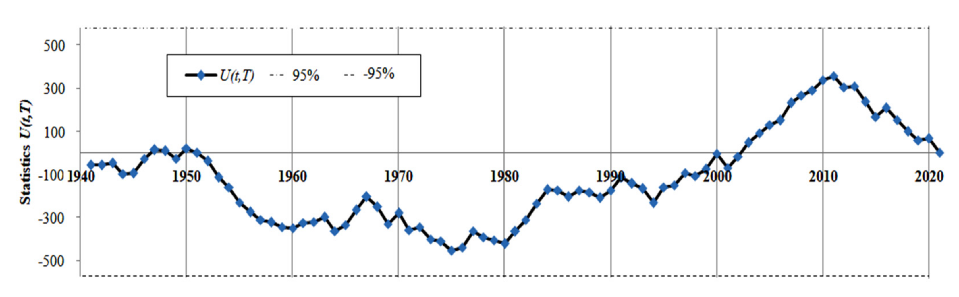
In addition,
Figure 3 presents the estimated Pettitt test statistic variable (
Ut,
T) over the years. In this graph, it is observed that the minimum value of the test (
Ut,
T = −459) occurred in 1975, whereas the highest value of the statistic occurred in 2011 (
Ut,
T=354).
The period between 1975 and 2011 included the highest observed values of the annual maximum daily flow, whose behaviour of the moving average (
Figure 2) was above the sample mean most of the time. During this time interval, the estimates of the Pettitt’s statistical variable sharply increased. From 2012 on, it was observed that there was a trend for the flow to decrease. However, as this recent period corresponded to only 10 years, it was not possible to safely estimate either the sample mean or the standard deviation. The precipitation observed in the 2012–2021 period was lower than that observed in the previous period (1976–2012), but it was not long enough for the robust determination of its statistical parameters. Thus, this 10-year period was incorporated into the long wet period (1976–2021*), even knowing that this inclusion would mean a reduction in the statistics for the wet period.
The ascending period of the statistical variable of the PT reflected, at each new reference value (
Yi), how it would be higher than the previous reference value, describing the ascending trend of the sequential observations (long wet period). The number of data that were lower than the reference value was higher, until it reached the upper limit, which showed the end of the wettest period. After that point, there was a curve inflection, and the number of flows observed in the series became lower than the previous reference, marking the beginning of the descending stretch and corresponding to the long driest period. The interpretation of the statistical variable behaviour of the Pettitt Test is a useful tool for identifying and separating the long dry and wet periods of the hydrological series.
Table 4 presents the results concerning the descriptive statistics of the maximum annual daily flow at different time intervals of the hydrological series. In addition to the sample mean and standard deviation (σ), the maximum and minimum observations are presented as well.
In
Table 3, we observe a great variability of the annual maximum daily flows over time. For the same hydrological series, the mean and standard deviation of the sample are not constant over time, making it possible to compare the values of different wet periods (1975 to 2011) and dry periods (time intervals from 1941 to 1975).
For the continuous long wet periods, as represented by the years 1975 to 2011, it is observed that besides the elevation of the sample mean, there was a significant increase in the sample standard deviation. Conversely, in long dry periods, there was a reduction in both the mean and the standard deviation regarding the estimates of the long wet periods.
Compared with the Gumbel–Chow mathematical model, thoroughly explained by Naghettini and Pinto [
32], the maximum probable flows could be estimated by the sum of the sample mean with the standard deviation multiplied by the frequency factor (
kt), which is a function of the recurrence interval
.
During the long wet period (1975–2021*), both descriptive statistics presented higher values; therefore, according to the Gumbel–Chow mathematical model [
32], it is expected that the estimates of maximum probable extreme flows are also higher when compared to the longest dry period [
37].
In the central south region of Brazil, a reduction in annual rainfall was observed from the middle of the year between 1930 and 1970, which concurred with a lower predominance of El Nino events. This was followed by the period 1975–2012, when there was greater predominance of ENSO [
38].
Analysing
Figure 2, the maximum extremes occurred. During the long wet period, the highest value (1376.6 m
3/s) was in 2007. However, in the long dry period, the lowest value (183.7 m
3/s) was reported in 1971.
Zuffo and Zuffo [
37] studied the historical series of annual precipitation of the City of Campinas, State of Sao Paulo from 1910 to 2014. They verified a great variability in precipitation over the years. The authors divided the hydrological series into four distinct plots to show that the mean and standard deviation of the sample were not constant over time. In the long dry periods of the study, there was a small drop in the average annual precipitation, but the major difference was in the standard deviation, which was much lower than those observed in the long wet periods, such as those represented by the years from 1910 to 1932 and from 1968 to 1991. Part of the study of Boulomytis et al. [
12] was also about the long wet and dry periods of the northern coastline of the State of Sao Paulo, analysing the hydrological data between 1940 and 2015. In this study, there were fluctuations in the wavelengths of the two different patterns of cycles for about 32 years.
According to Zuffo and Zuffo [
37] and Boulomytis at al. [
12], the analysis period significantly influences the results of the adjustment of theoretical models of probability distribution for extreme events since the traditional methods for estimating the parameters do not incorporate the cyclical rise and recession features of long periods and neither the change in mean nor standard deviation, which are essential parameters for defining the stochastic model.
In the current study, we corrected the
Qdmax values from the long dry period (1941–1975) to make the hydrological series unique and homogeneous, according to the proposed methodology. In
Figure 4, we observe the accumulated curves of the annual maximum daily flows as well as the respective linear regressions adjusted to remove cyclical trends and the final corrected curve.
After removing the temporal cyclical variability from the different periods, the parameters of the Gumbel probability distribution functions were adjusted to quantify the maximum probable flows as a function of the return period (
Tr).
Table 5 presents the estimates of the parameters of the theoretical Gumbel distribution function for the observed and corrected series. The corrected values of the mean, maximum and minimum observed are also updated.
Analysing the results of the Kolmogorov–Smirnov adherence test for the hydrological series in
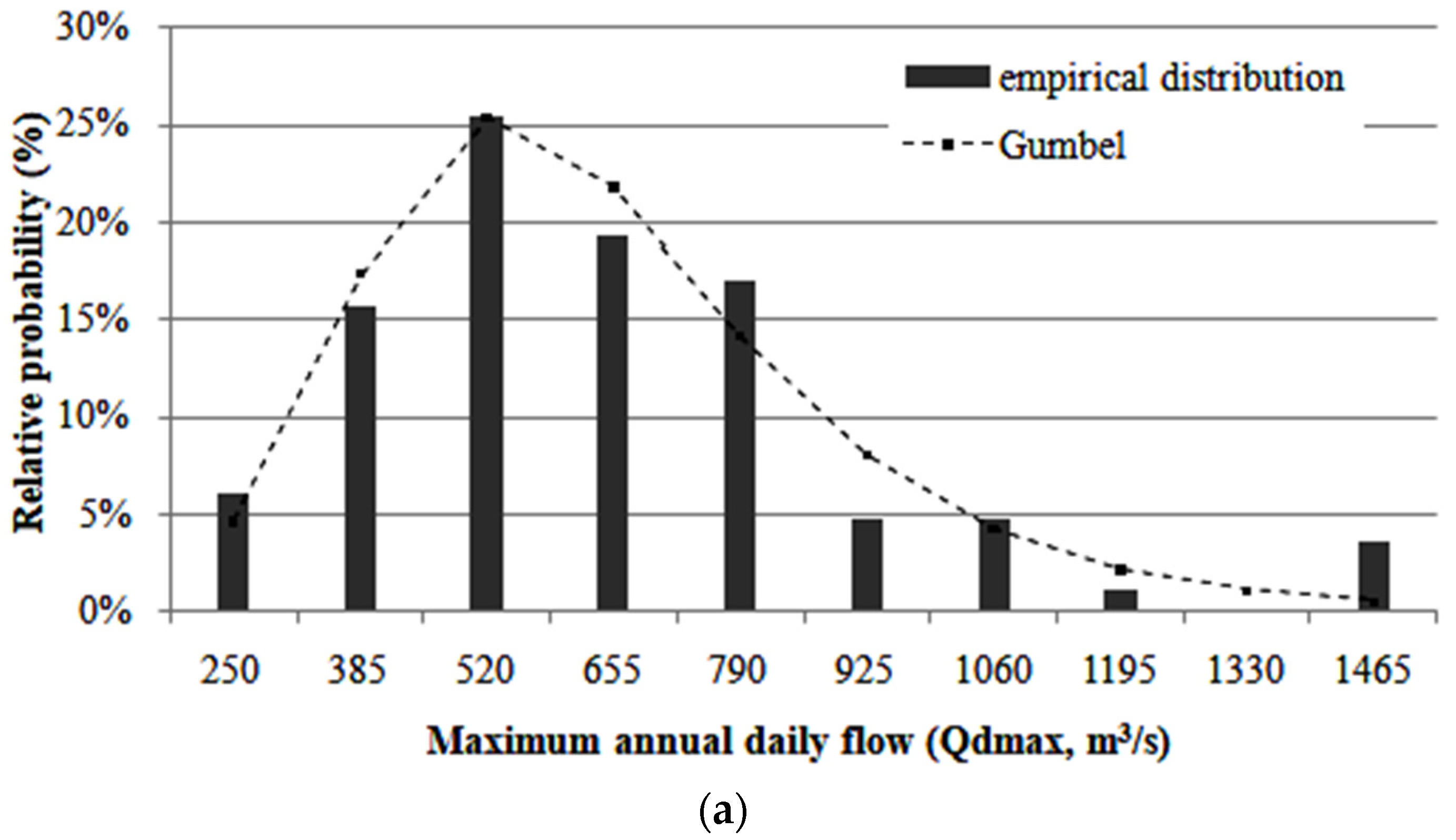
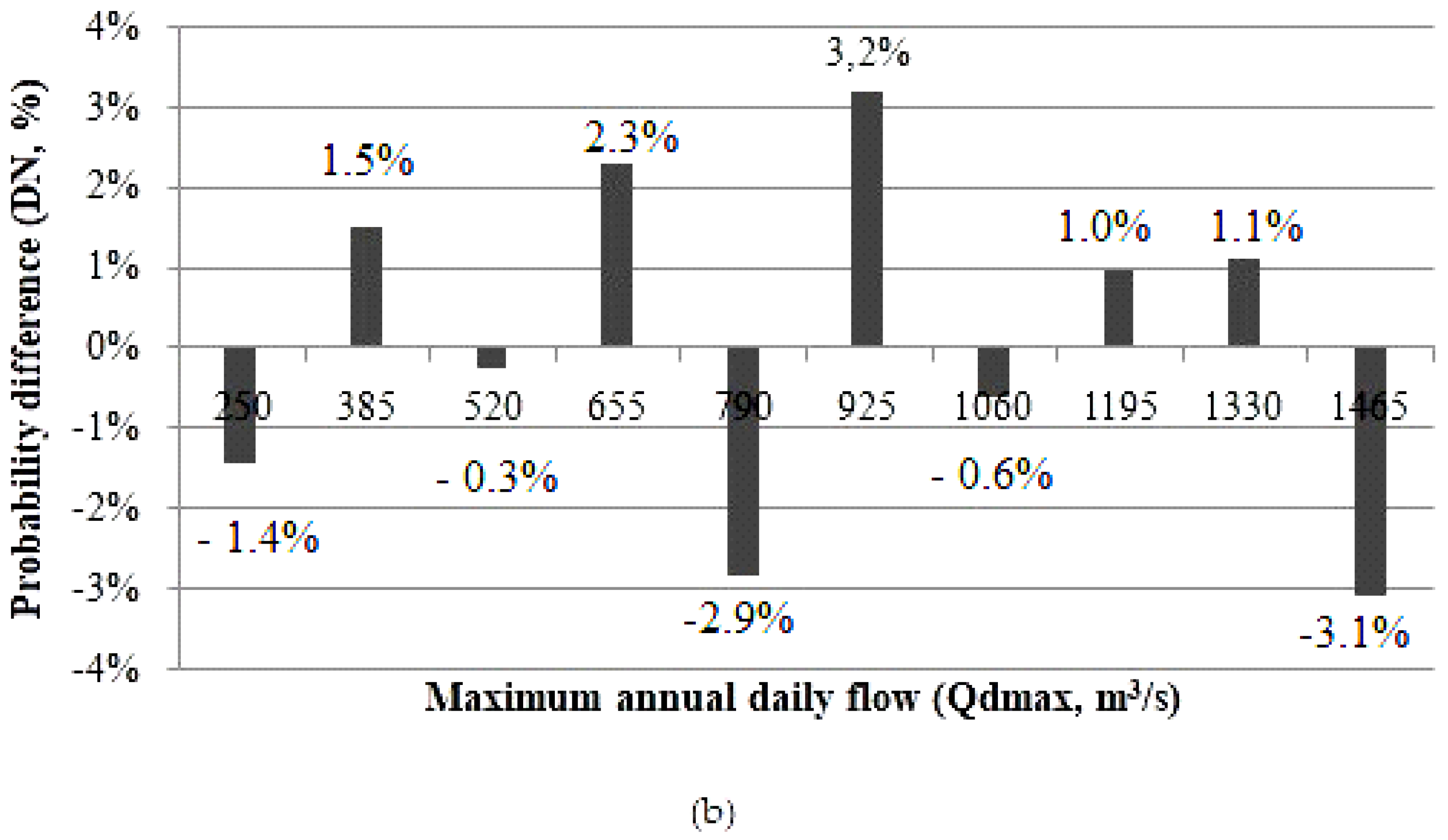
Table 5, it is possible to observe that both are adjusted to the theoretical distribution function. In
Figure 5 and
Figure 6, we present (a) the estimates of the partial frequencies and (b) the distance, or difference, between the theoretical and empirical probabilities for the observed and corrected historical hydrological series, respectively.
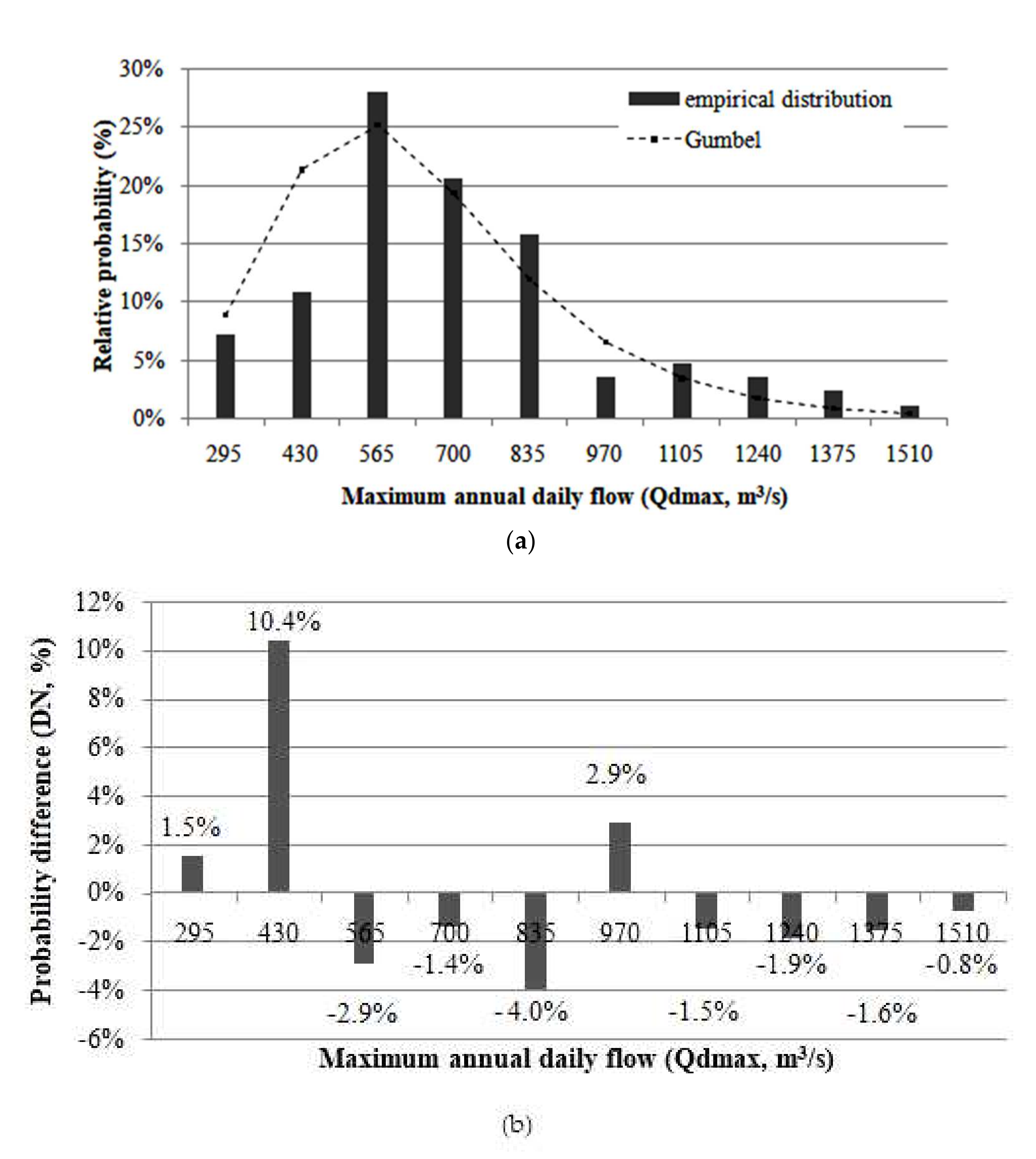
From the parameters of the theoretical Gumbel distribution function (
Table 5), the maximum probable annual daily flow rates were estimated for gauging station 4C-001 on the Pardo River. The results are presented in
Figure 7, where we compare the estimated maximum probable flows for the observed and corrected historical series.
The application of the proposed correction in the long dry period made it possible to homogenize the magnitude of the sample statistics (mean and standard deviation). Thus, the estimates of probable maximum flows were around 10% higher for the corrected historical series when compared to the observed historical series. If these corrections are not made, the hydraulic structures designed from the observed historical series could be insufficient throughout the years of the long wet period. Since this behaviour of decadal variations presents a certain periodicity, it is probable that other periods similar to the long dry and the wet periods will occur. Therefore, when designing the hydraulic structures, which consider maximum extreme events, two alternatives are recommended:
If the series is long enough and allows for separation into two subseries, one should comprise the long dry period and the other one, the long wet period.
If the series is not long enough, adopt the correction of the long dry period for the corresponding wet period, as proposed in this study.


 ,
, 


