Article

Analysis of the Distance between the Measured and Assumed Location of a Point Source of Pollution in Groundwater as a Function of the Variance of the Estimation Error

1
Faculty of Geotechnical Engineering, University of Zagreb, Hallerova aleja 7, 42000 Varaždin, Croatia
2
Department of Hydroscience and Engineering, Faculty of Civil Engineering, University of Zagreb, Fra Andrije Kačića-Miošića 26, 10000 Zagreb, Croatia
*
Author to whom correspondence should be addressed.
Hydrology 2023, 10(10), 199; https://doi.org/10.3390/hydrology10100199
Submission received: 1 August 2023 / Revised: 25 September 2023 / Accepted: 5 October 2023 / Published: 9 October 2023
(This article belongs to the Special Issue Groundwater Pollution: Sources, Mechanisms, and Prevention)

Abstract

:
The localization of pollution sources is one of the main tasks in environmental engineering. For this paper, models of spatial distribution of nitrate concentration in groundwater were created, and the point of highest concentration was determined. This point represents the assumed location of the pollution source and differs from the actual location, so there is a certain distance between the measured and assumed location. This paper puts forward a new hypothesis that the distance between the measured and the assumed location is a function of the variance of the estimation error. The scientific contribution of this paper is based on the fact that the interaction of statistical and geostatistical methods can locate the dominant point source of pollution or narrow down the search area. The above hypothesis is confirmed by the example of the Varaždin wellfield, which was closed due to an excessively high groundwater nitrate concentration. Seven different interpolation methods were used to create spatial distribution models. Each method provides a different model, a different variance of the estimation error, and estimates of the location of the pollution source. The smallest value of variance of the estimation error of 1.65 was obtained for the minimum curvature interpolation method and the largest value of variance (24.49) was obtained for the kriging with logarithmic variogram. Our results show a nonlinear and monotonic relationship between the distance and the variance of the estimation error, so logarithmic and rational quadratic models were fitted to the scatter point data. The models were linearized, a t-test was performed, and the results show that the models can be considered reliable, which is confirmed by the values of the coefficients of determination of the linearized models, which are around 0.50. The obtained results can be used in planning additional research work to determine the measured location of the pollution source. The research methodology we used is universal and can be applied to other locations where high concentrations of certain contaminants have been detected in groundwater in alluvial aquifers.

1. Introduction

Groundwater is the most abundant source of readily available freshwater in the world, excluding glaciers and polar ice caps, accounting for 97% of all freshwater [1]. For this reason, groundwater is now the most important source of water for various human needs. In the countries of the European Union, groundwater is estimated to meet 55% of domestic water needs [2], and when it comes to drinking water, the percentage increases to 75% [3]. With improvements in quality of life, high quality water is one of the necessary prerequisites for sustainable development [4], but in recent decades, there has been an increased emission of pollutants into the environment due to the increasingly rapid development of industry and agricultural production [5,6]. In this regard, groundwater is no exception, and its degradation is almost inevitable [7,8,9]. Global water demand has also been steadily increasing over the last three decades, and this trend is expected to continue [10]. In view of this, it is expected that new wellfields will be developed or that the pumping capacity of existing wells will be increased. As recent research has shown, the quality of groundwater can deteriorate when the pumping rate is increased [11].
Until recently, it was believed that the aquifer top deposits would provide sufficient protection to groundwater, but scientific studies and monitoring have shown that pollutants can easily penetrate the unsaturated zone and enter groundwater [12,13]. For this reason, groundwater quality and its changes in space and time have become the subject of numerous scientific studies. The first studies in this regard have shown that an increase in nitrate concentration is positively correlated with an increase in agricultural production on a global scale [14]. Recent studies also show that human activities are the main source of pollution of groundwater with nitrates [15]. Specifically, in order to increase agricultural land and improve conditions for food production, various melioration measures are applied. Studies show that the use of mineral fertilizers in agricultural production increases the nitrate concentration in groundwater [16,17,18,19]. For ease of access, agricultural lands are mostly located in the lowland catchment, which is a sensitive ecosystem with slow flow and a high groundwater table [20,21,22]. Due to these hydrogeological conditions, pollutants can easily penetrate from the surface into the subsurface, where they can persist for a long period of time. This leads to a violation of the natural balance between water and nutrients [23], and a significant correlation between agricultural development and groundwater quality degradation has been found [24,25,26,27,28].
An increased concentration of nitrates in drinking water negatively affects human health [29,30], and the toxicity of nitrates is a consequence of reducing nitrogen to nitrites [31]. Moreover, a high concentration of nitrites in the human body causes vasodilatory and cardiovascular disorders, while even a low concentration of nitrites can lead to methemoglobinemia, a disease which children are especially at risk of [32].
In the total concentration of nitrates in groundwater, one part refers to the natural contribution, the so-called nitrate background level (nbl), while the other part is related to the anthropogenic contribution. In one of the first studies in this field [33], indicative limits for nitrate concentrations in groundwater were presented, and they can be used to determine anthropogenic influence. The results of this particular study show that nitrate concentrations below 1 mg/L NO3 can be attributed to the natural nitrates of the aquifer, concentrations in the range of 1–13 mg/L NO3 can be characterized as a transitional range, i.e., concentrations that may or may not indicate an anthropogenic influence, and nitrate concentrations above 13 mg/L NO3 prove an anthropogenic influence. More recent studies also support these findings. For example, the value of nbl in the area of Rajasthan in India was estimated to be 7.2 mg/L [34], and in the Bono East regions in Ghana, nbl can be expected to be 3.9 mg/L [35]. For the area considered in this paper (a location in Northern Croatia), the Lepeltier method was used to determine nbl values of 8.6 + 2MAD (median absolute deviation) and 8.7 + 2SD (standard deviation) mg/L; thus, the upper limits of the assessment were estimated to be 18.2 mg/L and 24.3 mg/L, respectively [36].
Anthropogenic pollution sources can be divided into point and non-point sources in terms of their dispersion. Non-point sources of pollution represent dispersed sources on the surface. The most common examples of this type of pollution are agricultural lands treated with mineral fertilizers, and the most common type are nitrates, which are very persistent and mobile in groundwater. Although the concentrations in groundwater caused by this type of pollution can be relatively low, such sources can affect a large volume of groundwater due to their dispersion [37]. Point sources of pollution, on the other hand, refer to a localized area from which pollution is emitted. The concentration of pollution near point sources is usually high, but this type of pollution affects a smaller volume of groundwater. As the distance from the point source of pollution increases, the concentration of pollution in space decreases relatively rapidly [37]. Numerous studies have aimed to quantify the sources of pollution. In Koprivnica-Križevci County in Croatia, Nemcic Jurec et al. [38] show the impact of agricultural production as a point and non-point source of nitrate pollution in groundwater. Three different sites were investigated for possible pollution. At one site, where no pollution was expected and which also served as a control group, a very low nitrate concentration of 4.6 mg/L NO3 was determined. At the other two sites, an area of intensive agricultural production and a suburban area, the nitrate concentrations were found to be statistically significantly higher, with values of 28.7 and 26.5 mg/L NO3. As point sources of nitrate pollution in groundwater, some studies show increased nitrate concentrations in groundwater caused by poultry and livestock farming [39,40,41].
Interpolation methods are common techniques used in groundwater resource engineering and management. They can be used very effectively to determine groundwater levels, temperature variations, and the spatial distribution of certain types of pollution. There are several different methods, and the most commonly used are inverse distance weighting (idw), kriging, radial basis function, minimum curvature, and polynomial regression. The use of different interpolation methods can lead to different estimates regarding the parameter values at the interpolation points and, consequently, to the production of different maps presenting changes in the values of the analyzed parameters [42].
Kriging and idw methods were successfully used in the mapping of groundwater tables in the Erbil Basin in Iraq [43]. The authors processed data collected in 2004 and 2022 and concluded that the groundwater level dropped suddenly during this 18-year period. In a very recent study, a spatial interpolation method was used to detect the spatiotemporal dynamic patterns of groundwater level and salinity in the Yellow River delta in China [44]. The results showed that the risk of seawater intrusion into the local shallow aquifers in this region is high, as the mean groundwater level is lower than the local sea level in 42% of the region.
In a very recent study, interpolation methods were successfully used to determine the spatial distribution of temperature in shallow aquifers in Poland in the city of Wroclaw [45]. It was found that the spatial distribution of groundwater temperature for the analyzed period is characterized by higher temperatures in the city center. The best results were obtained using the Ordinary Kriging method. In other studies, interpolation methods based on point measurement data were also used to obtain groundwater temperatures for the analyzed areas [46,47], with particular emphasis on the kriging method [48,49].
As mentioned earlier, interpolation methods are used to map the distribution of pollution in groundwater. The inverse distance weighting method was used for the interpolation of heavy metals in groundwater in the Dehradun district in India [50], while the kriging method was used for the spatial interpolation of the water quality index in the Khyber Pakhtunkhwa province in Pakistan [51].
In this paper, statistical and geostatistical methods are presented to determine point source nitrate pollution in groundwater. Although numerical methods are being increasingly used nowadays, the advantage of the approach presented in this work is the simplicity and speed of the procedure. The development of a reliable numerical model requires detailed field research, which is often not possible due to time or cost constraints. For this reason, statistical and geostatistical methods remain an important tool in groundwater engineering and management. The location that is the focus of this article covers the narrow area of the Varaždin wellfield in the northern part of Croatia. This location was chosen because of the long-standing excessively high nitrate concentration in the groundwater, which is why the wellfield has been closed. Today, groundwater at this site is only used when other wellfields cannot meet the drinking water needs of the Varaždin water supply system. Recent investigations have shown that the majority of the pollution present in the area is attributable to the location being used as an illegal dumpsite for waste derived from poultry farms [41].
The very fact that the location of the dominant point pollution source is known provides an opportunity to test the hypothesis put forward in this work. This paper presents a novel hypothesis: the distance between the measured and assumed location (which can be determined via the use of interpolation methods) of the dominant point source of pollution is a function of the variance of the estimation error. Therefore, the scientific contribution of this paper is based on the fact that the dominant point source of pollution can be located and the fact that the search area can be narrowed down through the interaction of statistical and geostatistical methods. The results obtained have a very practical use, since the search area is narrowed down, which speeds up the search and reduces the associated costs. The method presented in this paper can be applied to other wellfields in alluvial aquifers where high concentrations of certain contaminants have been detected.

2. Materials and Methods
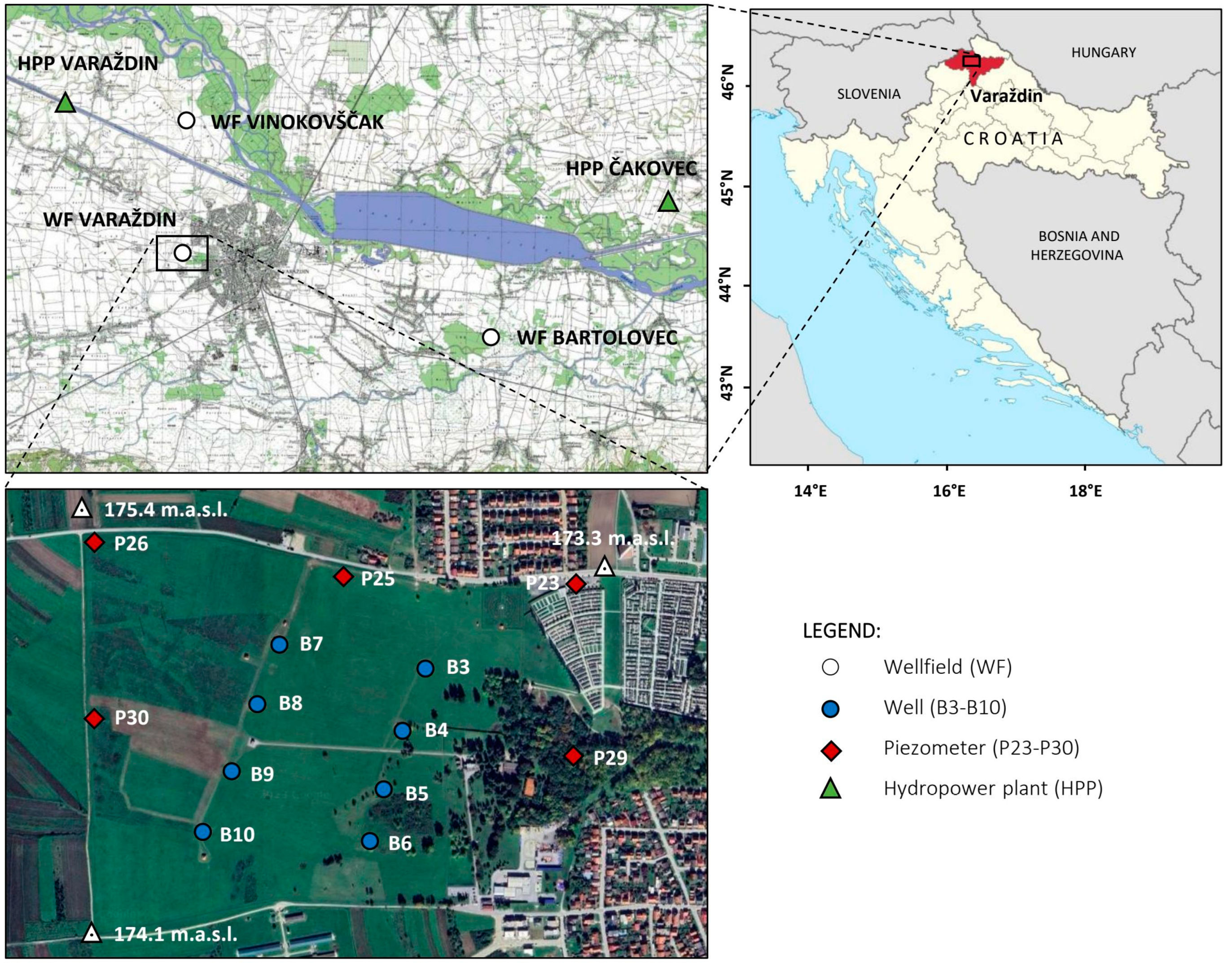
2.1. The Study Area

The study area is located in the north of the Republic of Croatia and includes the area of the Varaždin wellfield (Figure 1), which is located near the town of Varaždin. The Varaždin region is one of the most densely populated and economically developed areas in the Republic of Croatia. Groundwater for the Varaždin regional water supply system is pumped into the Varaždin, Bartolovec and Vinokovščak wellfields from the same alluvial aquifer, which is built of quaternary sand and gravel.
The Bartolovec and Vinokovščak wellfields are of good quality in terms of nitrate concentration, while the same does not apply for the Varaždin wellfield [52]. Therefore, in the Varaždin regional water supply network, the nitrate concentration was reduced by increasing the pumping rates in the Bartolovec and Vinokovščak wellfields [53]. Due to the high nitrate concentration, the Varaždin wellfield has not been active since 2004. For these reasons, the already existing problem in the water supply will soon become one of the main prerequisites for the sustainable development of the region and improvements to the quality of life of the region’s inhabitants.
The research scope of this work covers the period from 1993 to 2003 (until the closure of the Varaždin wellfield in 2004). Groundwater at the wellfield was regularly sampled from eight wells (B3–B10) and five piezometers (P23–P30) (Figure 1) from the upper aquifer layer during the observation period, so all results refer to this layer. A total of 3051 data points were collected, allowing for a reliable statistical analysis. Annual average values were calculated for each sampling point (well and piezometer), and these data were used in subsequent analyses (Table 1).
The geological structures of the aquifer consist of coarse-grained sediments of gravel and sand, while the underlying sediments consist of silt and clay. The thickness of the aquifer increases from west to east, and at the Varaždin wellfield it is about 75 m (Figure 2). The aquifer consists of two permeable gravel and sand layers, most of which are separated by a semipermeable aquitard of silt and clay [54]. The upper layer of the aquifer is composed of coarse-grained gravel and sand, while the lower part is mainly composed of fine-grained gravel with sand. The groundwater flows in a west–east direction, and it is parallel to the river Drava [55]. As previous investigations have shown, the quality of groundwater in the lower layer of the aquifer in the Bartolovec wellfield is significantly higher [56]. The values of hydraulic conductivity at the Varaždin wellfield were measured to be in the range of 185–241 m/day for the upper layer and 92.6 m/day for the lower layer [55].

2.2. Previous Research

For many years, the nitrate concentration in the Varaždin wellfield was higher than the maximum allowed concentration (MAC), according to the Ordinance on conformity parameters and analysis methods, monitoring and water safety plans for human consumption and according to the EU Nitrate Directive [57]. At the same time, the nitrate concentration in the groundwater at the other wellfields in the wider area of the town of Varaždin was much lower [56], which is adequately shown by the time series of the average annual nitrate concentrations of the wellfields (Figure 3). The curves represent the average annual nitrate concentration of all wells in the upper aquifer in each wellfield.
Several works have been written about the cause of such a high nitrate concentration in the Varaždin wellfield. The first works on this topic highlighted the application of mineral fertilizers as the main cause of such a high nitrate concentration in the groundwater [58]. Although this source of pollution contributes significantly to the total concentration of nitrates, in later works, through the use of numerical modeling methods, it was proved that the main cause of this problem is the illegal disposal of waste material from nearby poultry farms [39,41]. This source of pollution was classified as a point source of pollution.
As can be seen from Figure 3, the nitrate concentration varies significantly in terms of time and space. The construction of the Čakovec and Varaždin hydroelectric power plants (HPP) affected the quality of the groundwater. The influence of these power plants on the nitrate concentration was most evident. After the Varaždin HPP was put into operation in 1975, the groundwater level raised upstream. As a result, the nitrates deposited in the soil were washed away, which contributed to the increase in nitrate concentration in the groundwater [59]. The nitrate concentration in the groundwater increased steadily until 1982, when the reservoir of the Čakovec HPP was filled. The annual average curves at the Varaždin and Bartolovec wellfields then reached their maximum (Figure 3). Thereafter, the nitrate concentration at the wellfields decreased, and a constant decrease was recorded at the Bartolovec wellfield. The initial influence of HPPs gradually decreased, and today, it has completely disappeared [56].
However, as can be seen in Figure 3, the downward trend in the Varaždin wellfield was relatively short lived. The reason for this is the appearance of a new source of groundwater pollution, which had a dominant influence on nitrate concentrations. Since 1984, the average annual nitrate concentrations in the Varaždin wellfield have been in the range of 60 mg/L NO3 to 95 mg/L NO3, which is higher than MAC [56,60].
For this reason, the nitrate concentration at all of the groundwater sampling points in the wellfield (wells B3–B10 and piezometers P23–P30) was analyzed, and it was found that there are significant differences in nitrate concentration in the wells in the Varaždin wellfield: in some wells, the concentration is always higher (e.g., well B10), while in others (e.g., B3), it is always lower than the average value of the whole wellfield (Figure 4) [39]. This relationship was observed in all wells throughout the observation period. Since the nitrate concentration in the wells has such a regular relationship, we felt that our use of average nitrate concentrations in subsequent analyses was justified.

2.3. Aim of the Paper

One of the main tasks of environmental engineering is to determine the main sources of pollution. Therefore, in order to prevent further groundwater degradation, it is necessary to locate and eliminate them. Based on experimental data, it is possible to create a map with iso-lines of pollutant concentration in space by applying various interpolation methods. Such a map represents a 2D model of the spatial distribution of pollutants. The application of different interpolation methods leads to different results. Based on such a map, it is possible to assume the location of the pollution source, i.e., the point where the concentration is highest. However, any assessment may contain some error, i.e., the measured and the assumed location do not completely coincide, and there is a possibility that there is some difference between them. This difference was assumed to be proportional to the variance of the estimation error, and on this basis, the following null hypothesis was established:
The distance between the measured and the assumed location of the pollution source d is a function of the variance of the estimation error σ e r r o r 2 :
H 0 :                 d = d σ e r r o r 2  
That is, the assumed location with the smallest variance of the estimation error will be the closest to the measured location of the pollution source. An alternative hypothesis was also put forward:
H 1 :                 d d σ e r r o r 2  
Given that it is possible to obtain different models of the distribution of pollutants in space for the same experimental data, the goals of this work were as follows:
-
Based on the value of the variance of the estimation error, choose the interpolation method that gives the best estimate.
-
Based on the selected interpolation method, create a model that most closely approximates the actual spatial distribution of groundwater nitrate concentrations.
-
Use the created model to assume the location of the pollution source.
-
Determine the dependence of the distance between the measured and the assumed location on the variance of the estimation error and prove the hypothesis H0.
If the null hypothesis is correct, further investigation begin with the assumed location with the smallest error estimation. In this way, it is possible to reduce the area that must be investigated to find the measured location of the pollution source. The above hypothesis was tested at the Varaždin wellfield. In this wellfield, as mentioned above, the location of the point source of pollution has already been determined [41]. Therefore, this location was deemed suitable for testing the presented hypothesis.

2.4. Nitrate Field Analysis

Based on the spatial distribution of sampling locations and the corresponding average nitrate concentrations during the observed period, 2D models of the spatial distribution of nitrate concentration were created using several interpolation methods: (1) kriging, (2) minimum curvature, (3) polynomial regression, (4) radial basis function, (5) inverse distance to a power, (6) nearest neighbor, and (7) moving average. Since the kriging method is very commonly used for such purposes [61,62,63,64,65], an additional experimental variogram was constructed for this interpolation method, in which the following theoretical variograms were fitted: (a) linear, (b) linear with nugget, (c) power, (d) power with nugget, (e) logarithmic, (f) logarithmic with nugget, (g) gaussian, and (h) exponential (Figure 5). Hence, 14 different models were created. For each 2D model, the location of the point source of pollution was assumed, and the distances between the assumed and measured location d were determined. Golden Software Surfer 8.0 was used for this purpose.
Furthermore, for each interpolation method and theoretical variogram, the variance of the estimation error σ e r r o r 2 , which represents the average square of the difference between the measured and estimated values, was determined via a cross-validation procedure:
σ e r r o r 2 = 1 N i = 1 N z i z ^ i 2  
  • z i measured i-th value
  • z ^ i estimated i-th value
  • Ntotal number of measured values
For each model, the values of the variance of the estimation error and the corresponding distance between the measured and assumed location of the pollution source were determined. Based on these results, a dispersion diagram was created. With the models previously linearized, mathematical models were incorporated into this diagram and tested using the t-test:
t = r d f 1 r 2  
  • rcorrelation coefficient for the linearized model
  • df = N − 2, number of degrees of freedom
The obtained t values were compared with the critical value tα, which was determined based on the total number of data with a significance level of 5%. If t > tα, the model is considered reliable and the hypothesis H0 can be accepted:
t > t α H 0

3. Results and Discussion

The arithmetic mean nitrate concentrations at each sampling location in the observed period and the associated deviations obtained from each model are shown in Table 1. The smallest deviations were obtained for the radial basis function, kriging with linear and power variogram, and minimum curvature. Slightly larger deviations were obtained for kriging with logarithmic variogram and polynomial regression, while the largest deviations were obtained for inverse distance to a power.
The distances between the measured location of the point source of nitrate pollution according to [41] and the locations assumed by the interpolation methods used can be clearly seen in Figure 6. The results of all models show an increase in concentration in the northwest–southeast direction. However, for some methods, the highest concentration is within the model domain (kriging–linear variogram, kriging–linear variogram with nugget, kriging–power, kriging–power with nugget, kriging–logarithmic, kriging–logarithmic with nugget and radial basis function), while for others, this point is located at the very edge of the domain or, more precisely, at its origin (minimum curvature and polynomial regression). Moreover, the four methods used did not give good results (kriging–gaussian variogram, kriging–exponential variogram, nearest neighbor, and moving average) and it was not possible to determine the point with the highest nitrate concentration. Therefore, they can be characterized as methods that are not suitable for this type of analysis. For this reason, the results of these methods were not considered in subsequent analyses.
As expected, each of the interpolation methods and tested variograms resulted in a different spatial distribution of nitrate concentration and, accordingly, in a different value of the variance of the estimation error σ e r r o r 2 and the distance d between the measured and assumed location of the point source of nitrate pollution (Table 2). In other words, it can be recognized that the distance d is a function of the variance of the estimation error σ e r r o r 2 . As the value of the variance of the estimation error σ e r r o r 2 increases, the distance d also increases and vice versa. The smallest values of σ e r r o r 2 and d were obtained for the interpolation method minimum curvature, while the largest values were obtained for the kriging method with logarithmic variogram. In order to prove the hypothesis H0, a functional dependence σ e r r o r 2 (d) was interpolated using the data from Table 2, and the resulting approximation is shown in Figure 7. For this purpose, the program Statistica 13.5.0.17 TIBCO Software Inc. was used.
Figure 7a shows the fitted linear model, which calculated a coefficient of determination of only 0.36, indicating a low correlation between the two variables. In fact, from the distribution of the points with coordinates ( d , σ e r r o r 2 ), it can be seen that there is a non-linear and monotonic relationship between the mentioned variables. For this reason, the scatter point data ( d , σ e r r o r 2 ) were interpolated using the logarithmic model (Figure 7b):
d = a ln σ e r r o r 2 + b  
with parameters a = 78.76 and b = 188.31, and the modified rational quadratic model (Figure 7c):
d = a σ e r r o r 2 b + σ e r r o r 2  
with parameters a = 655.66 and b = 10.81. In order to prove hypothesis H0 using the t-test, the models given in Equations (6) and (7) need to be linearized. For this purpose, the functional dependency σ e r r o r 2 d for the logarithmic model can be expressed as follows:
σ e r r o r 2 = exp d b a  
and for the modified rational quadratic model, the same value can be expressed as follows:
σ e r r o r 2 = d b a d  
which yields the linear models illustrated in Figure 8 and characterized by coefficients of determination of R2 = 0.503 and R2 = 0.498, respectively.
Since the amount of available data points from Table 1 is 10, the number of degrees of freedom in the t-test is 8. Accordingly, the t-value for the linearized logarithmic model was determined to be 2.846, and for the modified rational quadratic model, the t-value was 2.818. These values should be considered with respect to the established critical value tα = 2.306. Since the obtained t values are higher than the critical value tα, the functional dependence σ e r r o r 2 d can be considered reliable for both models, confirming the assumption that the distance d between the measured and the predicted location of the point source of pollution is a function of the variance of the estimation error σ e r r o r 2 . In other words, it can be concluded that the following implication holds:
t > t α   H 0 : d = f σ e r r o r 2
Interpolation methods are very commonly used to evaluate groundwater level [66,67,68], temperature variations [45], and the spatial quality of various parameters. Kriging and idw are cited as the most commonly used methods [48,49]. Thus, the idw method has been used for the interpolation of heavy metals in groundwater in the Dehradun district in India [50], while the Kriging method has been used for the spatial interpolation of the water quality index in the Khyber Pakhtunkhwa province in Pakistan [51]. The results in this paper show that different spatial interpolation methods yield different maps from the same data, which is consistent with previous studies [69]. The results of previous studies also indicate that the Kriging interpolation method usually gives better results than the inverse distance to a power [70,71], and the results in this work confirm what has been said, which can clearly be seen from the deviation values shown in Table 1. The radial basis function method is also mentioned as a good method for determining the spatial distribution of nitrogen compounds in groundwater [42], and this is confirmed by the results obtained in this work, where the value of the variance of the estimation error was 2.94, while the deviation values at the control points were minimal.
Based on the smallest value of the variance of the estimation error, the minimum curvature method can be chosen as the best estimation method for a given data set. However, each site should be considered individually, and it is necessary to conduct studies at other sites to determine if this method provides the best results or if other methods would provide better results at other sites. However, the obtained result can be very useful to minimize the area where the source of pollution is suspected. Indeed, it is often the case that this source of pollution is not clearly visible at the surface of the considered aquifer, so the presented methodology can be used to reduce the search area. Since the smallest value of the variance of the estimation error is an indicator of the smallest distance d between the predicted and the measured (but unknown) location of the pollution source, the interpolation model with the smallest variance of the estimation error can be assumed to be the one that most closely resembles the actual spatial distribution of the pollution concentration, and the predicted location of the pollution source (with maximum pollution concentration values) can be used as a starting point for further investigations.

4. Conclusions

Based on measurements of groundwater pollution, our analysis showed that there is a functional dependence between the distance d between the measured and assumed locations of the point source of pollution, which were determined via the use of different interpolation methods, and the variance of the estimation error σ e r r o r 2 . The smallest value of the variance of the estimation error (1.65) was obtained for the minimum curvature interpolation method, which makes it the best estimate for a given dataset. On the other hand, the largest value, 24.49, was obtained for the kriging method–logarithmic variogram. Through using the three interpolation methods (moving average, nearest neighbor, kriging with gaussian and exponential variogram), it was not possible to determine the assumed location of the point source of pollution; therefore, these methods can be considered unsuitable for the given dataset. Each site should be considered individually because it is possible that, at other sites, a different interpolation method will give better results. To prove this, it is necessary to conduct this type of research at other locations. To verify the established hypothesis, the distance d between the maximum concentration in the model domain (assumed location of the nitrate pollution source) and the measured location of the nitrate pollution source was determined for each model. In addition, the variance of the estimation error σ e r r o r 2 was calculated for each of the tested methods, and the functional dependencies σ e r r o r 2 d were approximated by the logarithmic and modified rational quadratic models. Furthermore, the statistical t-test was used to confirm the established hypothesis. The results of the coefficients of determination of the linearized models are 0.50, and the obtained t values are higher than the critical value tα, so the models can be considered reliable at a 95% significance level. The results in this paper show that the interaction of statistical and geostatistical methods can successfully locate or reduce the search area of point sources of pollution. The obtained conclusion has a direct practical application. If the source of the groundwater pollution is not known in advance, considering that it is usually difficult to find on the aquifer surface (or even not located on the surface), a procedure to reduce the search area is necessary. The obtained conclusion can be used to define the origin of the search area as the point with the maximum pollutant concentration (obtained via an interpolation method that gives the minimal variance of the estimation error σ e r r o r 2 ). Accordingly, the search area can be narrowed down, and the search time can be shortened, which also leads to a reduction in the associated costs. Regarding future research, it is necessary to determine the influence of anisotropy on the spatial distribution of nitrate concentration in groundwater. If this influence is present, it is reasonable to assume that the variance of the estimation error could be further reduced. Consequently, the distance between the measured and predicted location of the pollution source would be reduced.

Author Contributions

Conceptualization, I.K. and M.Š.; methodology, I.K.; software, M.Š. and N.K.; validation, I.K., M.Š. and G.G.; formal analysis, I.K., M.Š. and N.K.; investigation, I.K. and N.K.; resources, G.G.; data curation, I.K. and M.Š.; writing—original draft preparation, I.K. and M.Š.; writing—review and editing, G.G.; visualization, M.Š.; supervision, I.K. and G.G.; funding acquisition, G.G. All authors have read and agreed to the published version of the manuscript.

Funding

This research received no external funding.

Data Availability Statement

The data used in this study are presented in the article. Additional data are available upon request from the corresponding author.

Conflicts of Interest

The authors declare no conflict of interest.

References

  1. Quevauviller, P.; Fouillac, A.M.; Grath, J.; Ward, R. Groundwater Monitoring; Wiley: Hoboken, NJ, USA, 2009. [Google Scholar] [CrossRef]
  2. EEA. Freshwater Quality—The European Environment—State and Outlook 2010; European Environment Agency: Copenhagen, Denmark, 2010. [Google Scholar]
  3. European Commission. Groundwater Protection in Europe: The New Groundwater Directive: Consolidating the EU Regulatory Framework; European Commission: Brussels, Belgium, 2009. [Google Scholar] [CrossRef]
  4. Alcamo, J. Water quality and its interlinkages with the Sustainable Development Goals. Curr. Opin. Environ. Sustain. 2019, 36, 126–140. [Google Scholar] [CrossRef]
  5. Neves, S.A.; Marques, A.C.; Patrício, M. Determinants of CO2 emissions in European Union countries: Does environmental regulation reduce environmental pollution? Econ. Anal. Policy 2020, 68, 114–125. [Google Scholar] [CrossRef]
  6. Wen, J.; Mughal, N.; Zhao, J.; Shabbir, M.S.; Niedbała, G.; Jain, V.; Anwar, A. Does globalization matter for environmental degradation? Nexus among energy consumption, economic growth, and carbon dioxide emission. Energy Policy 2021, 153, 112230. [Google Scholar] [CrossRef]
  7. Dyvak, M.; Rot, A.; Pasichnyk, R.; Tymchyshyn, V.; Huliiev, N.; Maslyiak, Y. Monitoring and Mathematical Modeling of Soil and Groundwater Contamination by Harmful Emissions of Nitrogen Dioxide from Motor Vehicles. Sustainability 2021, 13, 2768. [Google Scholar] [CrossRef]
  8. Kurwadkar, S.; Kanel, S.R.; Nakarmi, A. Groundwater pollution: Occurrence, detection, and remediation of organic and inorganic pollutants. Water Environ. Res. 2020, 92, 1659–1668. [Google Scholar] [CrossRef]
  9. Zhao, X.; Wang, D.; Xu, H.; Ding, Z.; Shi, Y.; Lu, Z.; Cheng, Z. Groundwater pollution risk assessment based on groundwater vulnerability and pollution load on an isolated island. Chemosphere 2022, 289, 133134. [Google Scholar] [CrossRef]
  10. Plessis, A.D. Water Resources from a Global Perspective. In South Africa’s Water Predicament; Springer: Cham, Switzerland, 2023; pp. 1–25. [Google Scholar] [CrossRef]
  11. Kovač, I.; Šrajbek, M.; Kranjčević, L.; Novotni-Horčička, N. Nonlinear models of the dependence of nitrate concentrations on the pumping rate of a water supply system. Geosci. J. 2020, 24, 585–595. [Google Scholar] [CrossRef]
  12. Das, B.; Pal, S.C. Assessment of groundwater vulnerability to over-exploitation using MCDA, AHP, fuzzy logic and novel ensemble models: A case study of Goghat-I and II blocks of West Bengal, India. Environ. Earth Sci. 2020, 79, 104. [Google Scholar] [CrossRef]
  13. Umar, M.; Khan, S.N.; Arshad, A.; Aslam, R.A.; Khan, H.M.S.; Rashid, H.; Pham, Q.B.; Nasir, A.; Noor, R.; Khedher, K.M.; et al. A modified approach to quantify aquifer vulnerability to pollution towards sustainable groundwater management in Irrigated Indus Basin. Environ. Sci. Pollut. Res. 2022, 29, 27257–27278. [Google Scholar] [CrossRef]
  14. Addiscott, T.M.; Whitmore, A.P.; Powlson, D.S. Farming, Fertilizers and the Nitrate Problem; Oxford University Press: Oxford, UK, 1991. [Google Scholar]
  15. Foster, S.; Hirata, R.; Andreo, B. The aquifer pollution vulnerability concept: Aid or impediment in promoting groundwater protection? Hydrogeol. J. 2013, 21, 1389–1392. [Google Scholar] [CrossRef]
  16. Almasri, M.N.; Kaluarachchi, J.J. Modular neural networks to predict the nitrate distribution in ground water using the on-ground nitrogen loading and recharge data. Environ. Model. Softw. 2005, 20, 851–871. [Google Scholar] [CrossRef]
  17. Farhadi, H.; Fataei, E.; Sadeghi, M.K. The Relationship Between Nitrate Distribution in Groundwater and Agricultural Land use (Case study: Ardabil Plain, Iran). Anthropog. Pollut. J. 2020, 4, 50–56. [Google Scholar]
  18. Srivastav, A.L. Chemical fertilizers and pesticides: Role in groundwater contamination. In Agrochemicals Detection, Treatment and Remediation; Elsevier: Amsterdam, The Netherlands, 2020; pp. 143–159. [Google Scholar] [CrossRef]
  19. Yu, L.; Zheng, T.; Yuan, R.; Zheng, X. APCS-MLR model: A convenient and fast method for quantitative identification of nitrate pollution sources in groundwater. J. Environ. Manag. 2022, 314, 115101. [Google Scholar] [CrossRef]
  20. Müller, L.; Behrendt, A.; Schindler, U. Strukturaspekte der bodendecke und bodeneigenschaften zweier niederungsstandorte in Nordostdeutschland: Structure aspects of the soil landscape and soil properties of two lowland sites in North-East Germany. Arch. Agron. Soil Sci. 2004, 50, 289–307. [Google Scholar] [CrossRef]
  21. Krause, S.; Bronstert, A.; Zehe, E. Groundwater–surface water interactions in a North German lowland floodplain—Implications for the river discharge dynamics and riparian water balance. J. Hydrol. 2007, 347, 404–417. [Google Scholar] [CrossRef]
  22. Schmalz, B.; Tavares, F.; Fohrer, N. Assessment of nutrient entry pathways and dominating hydrological processes in lowland catchments. Adv. Geosci. 2007, 11, 107–112. [Google Scholar] [CrossRef]
  23. Krause, S.; Bronstert, A. An advanced approach for catchment delineation and water balance modelling within wetlands and floodplains. Adv. Geosci. 2005, 5, 1–5. [Google Scholar] [CrossRef]
  24. Davey, I.R.; Besien, T.J.; Evers, S.; Ward, R. Nitrates in Groundwater—Agricultural Nitrate Contamination in Groundwater in England and Wales: An Overview; CRC Press: Boca Raton, FL, USA, 2014. [Google Scholar]
  25. He, X.-S.; Zhang, Y.-L.; Liu, Z.-H.; Wei, D.; Liang, G.; Liu, H.-T.; Xi, B.-D.; Huang, Z.-B.; Ma, Y.; Xing, B.-S. Interaction and coexistence characteristics of dissolved organic matter with toxic metals and pesticides in shallow groundwater. Environ. Pollut. 2020, 258, 113736. [Google Scholar] [CrossRef]
  26. Razowska-Jaworek, L.; Sadurski, A. Nitrates in Groundwater—Development of a Groundwater Abstraction Modelling Environment for Drinking Water Supply; CRC Press: Boca Raton, FL, USA, 2014. [Google Scholar]
  27. Sapek, B.; Sapek, A. Nitrates in Groundwater—Nitrate in Groundwater as an Indicator of Farmstead Impacts on the Environment; CRC Press: Boca Raton, FL, USA, 2014. [Google Scholar]
  28. Stockmarr, J.; Nyegaard, P. Nitrates in Groundwater—Nitrate in Danish Groundwater; CRC Press: Boca Raton, FL, USA, 2014. [Google Scholar]
  29. Li, P.; He, X.; Guo, W. Spatial groundwater quality and potential health risks due to nitrate ingestion through drinking water: A case study in Yan’an City on the Loess Plateau of northwest China. Hum. Ecol. Risk Assess. Int. J. 2019, 25, 11–31. [Google Scholar] [CrossRef]
  30. Yu, G.; Wang, J.; Liu, L.; Li, Y.; Zhang, Y.; Wang, S. The analysis of groundwater nitrate pollution and health risk assessment in rural areas of Yantai, China. BMC Public Health 2020, 20, 437. [Google Scholar] [CrossRef]
  31. Chambers, T.; Douwes, J.; Mannetje, A.; Woodward, A.; Baker, M.; Wilson, N.; Hales, S. Nitrate in drinking water and cancer risk: The biological mechanism, epidemiological evidence and future research. Aust. N. Z. J. Public Health 2022, 46, 105–108. [Google Scholar] [CrossRef] [PubMed]
  32. Brender, J.D. Human Health Effects of Exposure to Nitrate, Nitrite, and Nitrogen Dioxide. In Just Enough Nitrogen; Springer International Publishing: Cham, Switzerland, 2020; pp. 283–294. [Google Scholar] [CrossRef]
  33. Madison, R.J.; Brunett, J.O. Overview of the occurrence of nitrate in ground water in the United States. US Geol. Surv. Water-Supply Pap. 1984, 2275, 93–105. [Google Scholar]
  34. Rahman, A.; Mondal, N.C.; Tiwari, K.K. Anthropogenic nitrate in groundwater and its health risks in the view of background concentration in a semi arid area of Rajasthan, India. Sci. Rep. 2021, 11, 9279. [Google Scholar] [CrossRef] [PubMed]
  35. Manu, E.; Afrifa, G.Y.; Ansah-Narh, T.; Sam, F.; Loh, Y.S.A. Estimation of natural background and source identification of nitrate-nitrogen in groundwater in parts of the Bono, Ahafo and Bono East regions of Ghana. Groundw. Sustain. Dev. 2022, 16, 100696. [Google Scholar] [CrossRef]
  36. Nakić, Z.; Kovač, Z.; Parlov, J.; Perković, D. Ambient Background Values of Selected Chemical Substances in Four Groundwater Bodies in the Pannonian Region of Croatia. Water 2020, 12, 2671. [Google Scholar] [CrossRef]
  37. Eberts, M.; Thomas, M.A.; Jagucki, M.L. The Quality of Our Nation’s Waters: Factors Affecting Public-Supply-Well Vulnerability to Contamination: Understanding Observed Water Quality and Anticipating Future Water Quality; U.S. Department of the Interior, U.S. Geological Survey: Reston, VA, USA, 2013.
  38. Jurec, J.N.; Mesic, M.; Basic, F.; Kisic, I.; Zgorelec, Z. Nitrate concentration in drinking water from wells at three different locations in Northwest Croatia. Cereal Res. Commun. 2007, 35, 533–536. [Google Scholar] [CrossRef]
  39. Srajbek, M.; Kovac, I.; Novotni-Horcicka, N.; Kranjcevic, L. Assessment of average contributions of point and diffuse pollution sources to nitrate concentration in groundwater by nonlinear regression. Environ. Eng. Manag. J. 2020, 19, 95–104. [Google Scholar] [CrossRef]
  40. Kim, H.-R.; Yu, S.; Oh, J.; Kim, K.-H.; Lee, J.-H.; Moniruzzaman, M.; Kim, H.K.; Yun, S.-T. Nitrate contamination and subsequent hydrogeochemical processes of shallow groundwater in agro-livestock farming districts in South Korea. Agric. Ecosyst. Environ. 2019, 273, 50–61. [Google Scholar] [CrossRef]
  41. Šrajbek, M.; Kranjčević, L.; Kovač, I.; Biondić, R. Groundwater Nitrate Pollution Sources Assessment for Contaminated Wellfield. Water 2022, 14, 255. [Google Scholar] [CrossRef]
  42. Bronowicka-Mielniczuk, U.; Mielniczuk, J.; Obroślak, R.; Przystupa, W. A Comparison of Some Interpolation Techniques for Determining Spatial Distribution of Nitrogen Compounds in Groundwater. Int. J. Environ. Res. 2019, 13, 679–687. [Google Scholar] [CrossRef]
  43. Mustafa, J.S.; Mawlood, D.K. Mapping Groundwater Levels in Erbil Basin. Am. Sci. Res. J. Eng. Technol. Sci. 2023, 93, 21–38. [Google Scholar]
  44. Fan, X.; Min, T.; Dai, X. The Spatio-Temporal Dynamic Patterns of Shallow Groundwater Level and Salinity: The Yellow River Delta, China. Water 2023, 15, 1426. [Google Scholar] [CrossRef]
  45. Hajnrych, M.; Blachowski, J.; Worsa-Kozak, M. Study of groundwater temperature spatio-temporal variation in the city of Wroclaw. Preliminary results. IOP Conf. Ser. Earth Environ. Sci. 2023, 1189, 012028. [Google Scholar] [CrossRef]
  46. Lubis, R.F.; Yamano, M.; Delinom, R.; Martosuparno, S.; Sakura, Y.; Goto, S.; Miyakoshi, A.; Taniguchi, M. Assessment of urban groundwater heat contaminant in Jakarta, Indonesia. Environ. Earth Sci. 2013, 70, 2033–2038. [Google Scholar] [CrossRef]
  47. Taniguchi, M.; Shimada, J.; Fukuda, Y.; Yamano, M.; Onodera, S.-I.; Kaneko, S.; Yoshikoshi, A. Anthropogenic effects on the subsurface thermal and groundwater environments in Osaka, Japan and Bangkok, Thailand. Sci. Total Environ. 2009, 407, 3153–3164. [Google Scholar] [CrossRef] [PubMed]
  48. Previati, A.; Crosta, G.B. Characterization of the subsurface urban heat island and its sources in the Milan city area, Italy. Hydrogeol. J. 2021, 29, 2487–2500. [Google Scholar] [CrossRef]
  49. Benz, S.A.; Bayer, P.; Goettsche, F.M.; Olesen, F.S.; Blum, P. Linking Surface Urban Heat Islands with Groundwater Temperatures. Environ. Sci. Technol. 2016, 50, 70–78. [Google Scholar] [CrossRef]
  50. Nayak, A.; Matta, G.; Uniyal, D.P.; Kumar, A.; Kumar, P.; Pant, G. Assessment of potentially toxic elements in groundwater through interpolation, pollution indices, and chemometric techniques in Dehradun in Uttarakhand State. Environ. Sci. Pollut. Res. 2023. [Google Scholar] [CrossRef]
  51. Khan, M.; Almazah, M.M.A.; EIlahi, A.; Niaz, R.; Al-Rezami, A.Y.; Zaman, B. Spatial interpolation of water quality index based on Ordinary kriging and Universal kriging. Geomat. Nat. Hazards Risk 2023, 14, 2190853. [Google Scholar] [CrossRef]
  52. Kovač, I.; Kovačev-Marinčić, B.; Novotni-Horčička, N.; Mesec, J.; Vugrinec, J. Komparativna analiza koncentracije nitrata u gornjem i donjem sloju varaždinskog vodonosnika. Rad. Zavoda Znan. Varaždin 2017, 28, 41–57. [Google Scholar] [CrossRef]
  53. Novotni-Horčička, N.; Šrajbek, M.; Kovač, I. Nitrati u Regionalnom vodovodu Varaždin. In Voda i Javna Vodoopskrba; Hrvatski Zavod za Javno Zdravstvo (HZJZ): Zagreb, Croatia, 2010; pp. 123–131. [Google Scholar]
  54. Urumović, K. O kvartnom vodonosnom kopleksu u području Varaždina. Geološki Vjesn. 1971, 43, 109–118. [Google Scholar]
  55. Larva, O. Aquifer Vulnerability at Catchment Area of Varaždin Pumping Sites. Ph.D Thesis, Faculty of Mining, Geology and Petroleum Engineering, University of Zagreb, Zagreb, Croatia, 2008. [Google Scholar]
  56. Šrajbek, M. Nitrate Pollution Propagation in Groundwater and Wellfield Imapct Assessment. Ph.D Thesis, Faculty of Engineering, University of Rijeka, Rijeka, Croatia, 2021. [Google Scholar]
  57. European Union. Council Directive 91/676/EEC of 12 December 1991 concerning the protection of waters against pollution caused by nitrate from agricultural sources. Off. J. Eur. Commun. 1991, 375, 1–13. [Google Scholar]
  58. Gjetvaj, G. Identifikacija porijekla nitrata u podzemnim vodama Varaždinske regije. Hrvat. Vode 1993, 1, 247–252. [Google Scholar]
  59. Grđan, D.; Durman, P.; Kovačev-Marinčić, B. Odnos promjene režima i kvalitete podzemnih voda na crpilištima Varaždin i Bartolovec. Geološki Vjesn. 1991, 44, 301–308. [Google Scholar]
  60. Kovač, I. Statistical-Variographic Analysis of Ground Water Chemical Composition in Varaždin Region. Ph.D. Thesis, Faculty of Minning, Geology and Petroleum Engineering, University of Zagreb, Zagreb, Croatia, 2004. [Google Scholar]
  61. Arslan, H. Spatial and temporal mapping of groundwater salinity using ordinary kriging and indicator kriging: The case of Bafra Plain, Turkey. Agric. Water Manag. 2012, 113, 57–63. [Google Scholar] [CrossRef]
  62. Thomas, E.O. Spatial evaluation of groundwater quality using factor analysis and geostatistical Kriging algorithm: A case study of Ibadan Metropolis, Nigeria. Water Pract. Technol. 2023, 18, 592–607. [Google Scholar] [CrossRef]
  63. Belkhiri, L.; Tiri, A.; Mouni, L. Spatial distribution of the groundwater quality using kriging and Co-kriging interpolations. Groundw. Sustain. Dev. 2020, 11, 100473. [Google Scholar] [CrossRef]
  64. Gundogdu, K.S.; Guney, I. Spatial analyses of groundwater levels using universal kriging. J. Earth Syst. Sci. 2007, 116, 49–55. [Google Scholar] [CrossRef]
  65. Rostami, A.A.; Karimi, V.; Khatibi, R.; Pradhan, B. An investigation into seasonal variations of groundwater nitrate by spatial modelling strategies at two levels by kriging and co-kriging models. J. Environ. Manag. 2020, 270, 110843. [Google Scholar] [CrossRef]
  66. Arkoc, O. Modeling of spatiotemporal variations of groundwater levels using different interpolation methods with the aid of GIS, case study from Ergene Basin, Turkey. Model. Earth Syst. Environ. 2022, 8, 967–976. [Google Scholar] [CrossRef]
  67. Varouchakis, A.; Hristopulos, D.T. Comparison of stochastic and deterministic methods for mapping groundwater level spatial variability in sparsely monitored basins. Environ. Monit. Assess. 2013, 18, 1–19. [Google Scholar] [CrossRef] [PubMed]
  68. Xiao, Y.; Gu, X.; Yin, S.; Shao, J.; Cui, Y.; Zhang, Q.; Niu, Y. Geostatistical interpolation model selection based on ArcGIS and spatio-temporal variability analysis of groundwater level in piedmont plains, northwest China. Springerplus 2016, 5, 425. [Google Scholar] [CrossRef] [PubMed]
  69. Elumalai, V.; Brindha, K.; Sithole, B.; Lakshmanan, E. Spatial interpolation methods and geostatistics for mapping groundwater contamination in a coastal area. Environ. Sci. Pollut. Res. 2017, 24, 11601–11617. [Google Scholar] [CrossRef]
  70. Ahmad, A.Y.; Saleh, I.A.; Balakrishnan, P.; Al-Ghouti, M.A. Comparison GIS-Based interpolation methods for mapping groundwater quality in the state of Qatar. Groundw. Sustain. Dev. 2021, 13, 100573. [Google Scholar] [CrossRef]
  71. Mirzaei, R.; Sakizadeh, M. Comparison of interpolation methods for the estimation of groundwater contamination in Andimeshk-Shush Plain, Southwest of Iran. Environ. Sci. Pollut. Res. 2016, 23, 2758–2769. [Google Scholar] [CrossRef]
Figure 1. Geographical position of the Varaždin wellfield and spatial arrangement of wells and piezometers.
Hydrology 10 00199 g001
Figure 2. Three-dimensional model of the wider area of the Varaždin wellfield [41].
Hydrology 10 00199 g002
Figure 3. Time series of the annual average nitrate concentrations in the wellfields in Bartolovec, Varaždin, and Vinokovščak.
Hydrology 10 00199 g003
Figure 4. Annual average nitrate concentration curves in groundwater at the Varaždin wellfield in wells B3, B10, and the wellfield annual average.
Hydrology 10 00199 g004
Figure 5. Experimental variograms in kriging interpolation method.
Hydrology 10 00199 g005
Figure 6. Maps of isolines of nitrate concentration in groundwater made based on various interpolation methods and the assumed location of the source of pollution.
Hydrology 10 00199 g006aHydrology 10 00199 g006bHydrology 10 00199 g006cHydrology 10 00199 g006d
Figure 7. The approximated functional dependency σ e r r o r 2 d based on (a) a linear model, (b) a logarithmic model, and (c) a modified rational quadratic model.
Hydrology 10 00199 g007
Figure 8. Graphical representation of the linearized logarithmic and modified rational quadratic models given by Equations (8) and (9).
Hydrology 10 00199 g008
Table 1. Numerical means regarding nitrate concentration at control points and deviation values obtained via the use of interpolation methods.
B3B4B5B6B7B8B9B10P23P25P26P29P30∑Δ2 Δ 2 ¯
Average
[mg/L NO3]
74.1475.3576.780.0476.7181.4285.9287.8065.0371.6777.468.6287.00
Kriging–linear0.060.01−0.05−0.02−0.020.020.100.02−0.03−0.05−0.06−0.040.040.030.00
Kriging–linear nugget0.060.01−0.05−0.02−0.020.030.100.02−0.03−0.05−0.06−0.040.030.030.00
Kriging–power0.120.03−0.09−0.01−0.050.050.210.08−0.12−0.12−0.14−0.110.110.150.01
Kriging–power nugget0.120.03−0.10−0.03−0.040.060.200.08−0.12−0.11−0.13−0.110.100.140.01
Kriging–logarithmic−0.07−0.18−0.280.61−0.400.692.161.43−2.70−1.29−0.56−1.991.9024.681.90
Kriging–logarithmic nugget−0.02−0.14−0.250.52−0.340.561.860.98−2.20−1.06−0.46−1.681.5116.531.27
Minimum curvature−0.01−0.10−0.100.060.03−0.040.010.00−0.250.030.080.240.010.150.01
Polynomial regression1.72−0.24−1.84−1.56−0.331.142.521.251.67−0.21−2.52−1.870.2730.922.38
Radial basis function0.000.00−0.010.000.000.000.010.000.000.000.000.000.000.000.00
Inverse distance to a power−5.50−7.79−7.90−2.87−0.95−0.771.054.46−9.21−1.784.81−16.253.65572.6344.05
Table 2. Values of the variance of the estimation error σ e r r o r 2 and the distance d between the measured and predicted location of the point source of nitrate pollution.
Interpolation Method
σ e r r o r 2
[(mg/L)2]
d
[m]
Kriging–linear variogram4.13466.61
Kriging–linear variogram with nugget4.12463.41
Kriging–power variogram5.66594.50
Kriging–power variogram with nugget5.62594.35
Kriging–logarithmic variogram24.49596.12
Kriging-logarithmic variogram with nugget23.44595.81
Kriging–gaussian variogram51.87not applicable
Kriging–exponential variogram51.87not applicable
Minimum curvature1.650.00
Polynomial regression2.380.00
Radial basis function2.94309.88
Inverse distance to a power22.33594.74
Nearest neighbor22.26not applicable
Moving average23.01not applicable
Disclaimer/Publisher’s Note: The statements, opinions and data contained in all publications are solely those of the individual author(s) and contributor(s) and not of MDPI and/or the editor(s). MDPI and/or the editor(s) disclaim responsibility for any injury to people or property resulting from any ideas, methods, instructions or products referred to in the content.

