Nutrient Loadings to Utah Lake from Precipitation-Related Atmospheric Deposition

Abstract

Atmospheric deposition (AD) is a less understood and quantified source of nutrient loading to waterbodies. AD occurs via settling (large particulates), contact (smaller particulates and gaseous matter), and precipitation (rain, snow) transport pathways. Utah Lake is a shallow eutrophic freshwater lake located in central Utah, USA, with geophysical characteristics that make it particularly susceptible to AD-related nutrient loading. Studies have shown AD to be a significant contributor to the lake’s nutrient budget. This study analyzes nutrient samples from nine locations around the lake and four precipitation gauges over a 6-year study period using three different methods to estimate AD from the precipitation transport pathway. The methods used are simple averaging, Thiessen polygons, and inverse distance weighting, which we use to spatially interpolate point sample data to estimate nutrient lake loads. We hold that the inverse distance weighting method produces the most accurate results. We quantify, present, and compare nutrient loads and nutrient loading rates for total phosphorus (TP), total inorganic nitrogen (TIN), and ortho phosphate (OP) from precipitation events. We compute loading rates for the calendar year (Mg/yr) from each of the three analysis methods along with monthly loading rates where Mg is 10⁶ g. Our estimated annual precipitation AD loads for TP, OP, and TIN are 120.96 Mg/yr (132.97 tons/yr), 60.87 Mg/yr (67.1 tons/yr), and 435 Mg/yr (479.5 tons/yr), respectively. We compare these results with published data on total AD nutrient loads and show that AD from precipitation is a significant nutrient source for Utah Lake, contributing between 25% and 40% of the total AD nutrient load to the lake.

1. Introduction

1.1. Atmospheric Deposition of Nutrients to Lakes and Reservoirs

Characterizing nutrient loads to water bodies is critical for informed management [1] and for making often costly decisions related to minimizing these loads. Excess nutrients cause issues such as excessive algal growth, which can cause low-oxygen (i.e., hypoxic) conditions and, depending on the species, toxic water conditions [2]. The detrimental impacts of algal blooms have been identified in lakes and reservoirs throughout the world [3,4,5].

While concern regarding harmful algal blooms (HABs) has grown globally [6,7], the occurrence of substantial algal blooms, a characteristic of eutrophic conditions [7,8], is not a recent development in Utah Lake [8]. Nutrient inputs into Utah Lake encompass a range of sources, including wastewater treatment plants (WWTPs), streams, overland runoff, sediment, biological contributors (such as carp), atmospheric deposition, geochemical mechanisms, and urban runoff [9,10,11,12]. It is estimated that more than 95% of these nutrient inputs remain within Utah Lake, suggesting that the concentrations of nutrients within the water column are likely regulated by a variety of geochemical processes rather than direct influent loads [13,14].

Understanding, quantifying, and characterizing these loads are important. Nutrient loads from atmospheric deposition are often not considered in nutrient budgets but can be substantial [15,16,17,18]. This study presents a new data set that we use to both quantify and characterize nutrient deposition to Utah Lake associated with precipitation events.

1.2. Utah Lake Location and Setting

Utah Lake, a remnant of the Pleistocene Lake Bonneville, is a shallow eutrophic freshwater lake approximately 50 km (30 miles) long and 10 km (6 miles) wide [13] and located in Utah County, Utah, USA. When full, the surface area of the lake is roughly 40,000 ha (95,000 acres), with an average depth of 2.8 m (9.2 feet) [13]. Due to its large surface-area-to-volume ratio, the lake is susceptible to atmospheric deposition (AD) of nutrients [10,11]. The lake is considered highly eutrophic by the Larsen–Mercier Tropic State model and moderately eutrophic by the Carlson Trophic State Index model [13]. The lake is commonly used for recreation but has been temporarily closed at times due to the presence of harmful algal blooms [14,19].

The Utah Division of Water Quality (DWQ) has recently elevated its interest in the nutrient loadings to the lake and is studying the impacts of reducing wastewater treatment plant (WWTP) nutrient discharge limits and other mitigation efforts [13,20]. The proposed mitigation efforts assume that phosphorus loadings from anthropogenic sources are a significant contribution to the lake’s overall nutrient budget [20,21].

Research has shown that for Utah Lake, natural sources such as atmospheric deposition and sediments could provide significant contributions in addition to more commonly studied sources, such as nutrient inflows from rivers and streams and anthropogenic sources such as waste water treatment plants. Abu-Hmeidan et al. [21] found that “natural phosphorous loadings could be a significant factor, and that the impaired state of the lake may be relatively insensitive to external anthropogenic loadings”, while Randall et al. [14] found that sediment nutrient recycling could control water column nutrient concentrations. Barrus et al. [10] extended the study by Olsen et al. [11], using data measured around Utah Lake to address the uncertainty and criticism of some sampling methods.

Zheng et al. [22] showed that nitrogen (N) and phosphorous (P) are the major nutrients transported to waterbodies through AD. Utah Lake is particularly sensitive to nutrient loads because of its shallow depth and large surface area: the ratio of surface to volume is high, with typical average depths in the order of 2 to 3 m and a surface area of 400 million m² (40,000 ha) [19]. Utah Valley, where Utah Lake is located, experiences strong summer inversions that result in high particulate matter concentrations, which contribute to AD during precipitation events and through contact with the lake surface (dry deposition) [10]. Soils in the area have phosphorus concentrations in the order of 1000 mg/kg, much of which is available to the water column when these solids are deposited as dust [14,21,23].

1.3. Previous Work on Utah Lake AD

In 2018, the Utah Division of Water Quality (DWQ) established the Utah Lake Science Panel (ULSP) which “… is charged with guiding the development of site-specific nitrogen and phosphorus criteria that are protective of the aquatic life, recreational, and agricultural uses of the lake” [24]. The ULSP reviewed several AD studies estimating loads to Utah Lake and determined that the majority of the data from two large multi-year field sampling efforts [10,25] that directly measured AD near the shore of Utah Lake should be excluded [26]. As of this writing, the ULSP is considering total P AD loads in the range of 27 to 45 Mg/yr (kg∙10³/yr) (30 to 50 tons/yr), significantly lower than either of the two published field campaigns, which used measured data around the lake and estimated P loads from 91 to 227 Mg/yr (100 to 250 tons/yr), depending on assumptions, from all AD sources [10,25], where Mg is 10³ kg or 10⁶ g.

Our definitions, which are needed to match our sampling methods, are different from traditional definitions. Therefore, we use three categories to classify AD to water bodies based on the different deposition processes: settlement (dust), contact, and precipitation (or washout). These categories are different to traditional AD research which defines wet (gases washed out during precipitation), dry (settled dust and particulates), and bulk (a combination of the wet and dry processes) categories. We separate precipitation deposition as a separate category because the samples we use in this study include particulate matter in the atmosphere at the time of precipitation but do not include dust deposition outside of precipitation events. Thus, it is different from traditional definitions of either bulk or wet deposition. We define our three processes as follows:

• Settlement deposition occurs when large particles (10–100 µm), which are transported by strong wind and other disturbances, leave the atmosphere due to gravity. If they settle on the ground, they are only resuspended by wind or mechanical action.
• Contact deposition occurs when smaller particles, less than 10 µm, and especially less than 2.5 µm, are deposited when they contact a surface and “stick” because of electrostatic charge or moisture. Because of their size, these particles do not generally settle but move through advection and Brownian motion and are easily kept aloft by slight breezes or resuspended if they are not attached to a surface. Through movement, they contact surfaces. Dry surfaces soon become “saturated”, so that additional particles either are not captured or displace an existing particle, while wet surfaces, such as lakes, capture particles that stick to the water surface by mixing them into the water column. Contact deposition includes gases which dissolve into water and are captured.
• Precipitation (or washout) deposition refers to nutrients that are washed out of the atmosphere during a precipitation event. This includes dust (>10 µm), fines (<10 µm), and gases.

1.4. Study Overview

We present collected data and associated analyses to quantify loading rates for atmospheric deposition to Utah Lake. Our samples mainly measure AD from the precipitation deposition process. The rainfall gauges used did capture some settlement deposition, but the samplers were not designed to capture dust particles. In periods between precipitation events, the samplers did capture some dry deposition, but again, the samplers were not designed to retain these small particulates, and we assume the contribution is minimal. While dry deposition can be significant to wet surfaces, such as a lake, dry deposition on dry solid surfaces is minimal. We acknowledge that while our data generally represent precipitation deposition, they do include certain settlement and dry deposition components. As such, the loads and rates computed using these data can be considered a lower bound for nutrient AD from all sources to Utah Lake.

We present an analysis of six years of precipitation samples collected at nine locations around the lake using three different analysis approaches. We compute estimated loads and loading rates for total phosphorus (TP), total inorganic nitrogen (TIN), and ortho phosphate (OP). This analysis uses data first reported in a master’s thesis [25].

This study aims to characterize and quantify AD of nutrients to Utah Lake associated with precipitation events. Our goal is to better comprehend nutrient loadings in the context of management decisions aimed at reducing nutrient inflows and understanding the impact of these reductions. If AD is large compared with potential reductions, impacts will be smaller. For other regions, this study offers a relatively straightforward method for estimating nutrient AD from precipitation that only requires collecting precipitation samples and measuring nutrient concentrations. However, it is crucial to note that this method does not encompass the entire spectrum of nutrient AD loading.

2. Materials and Methods

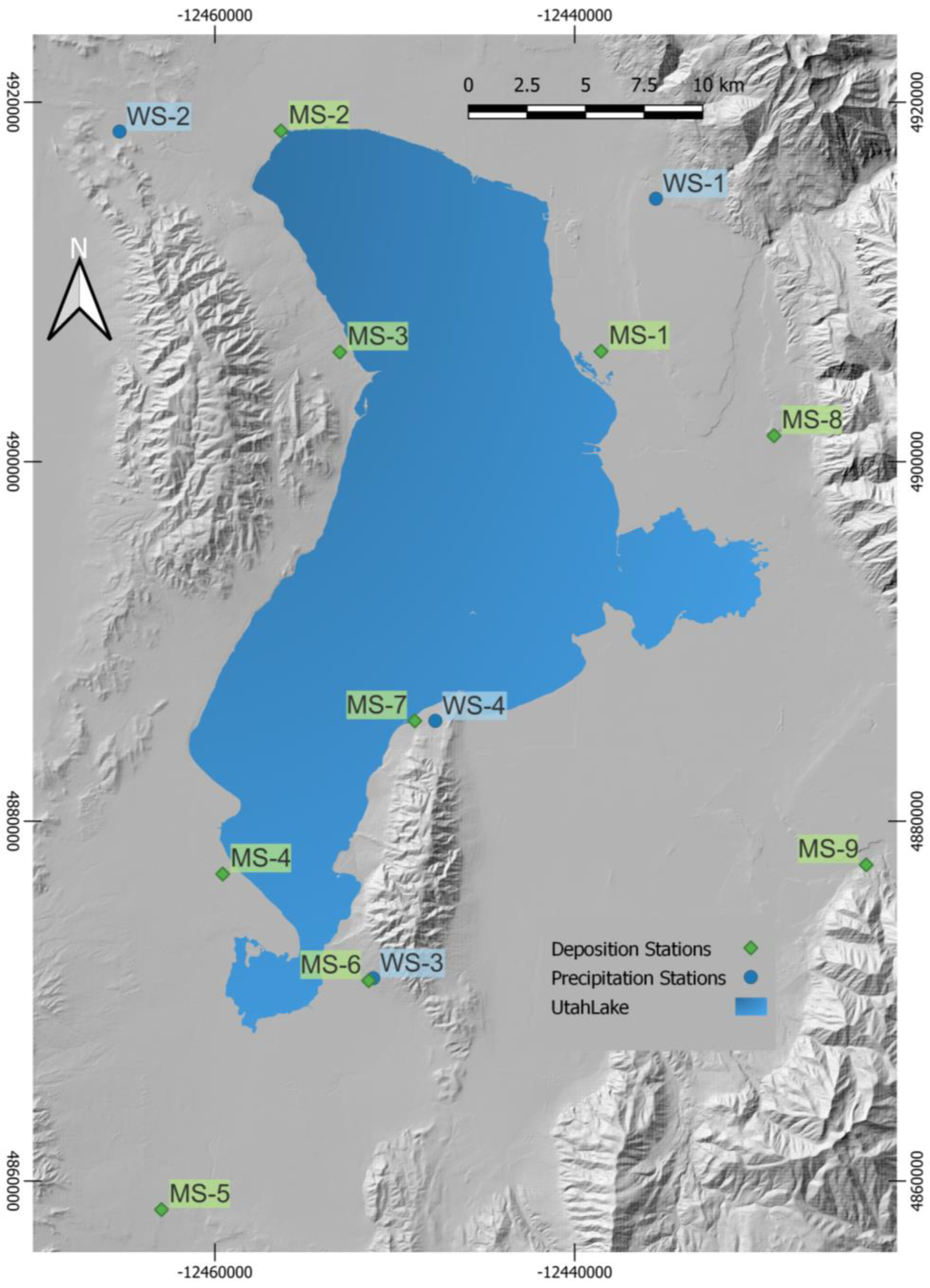
2.1. Sample Collection and Method Overview

Beginning in October 2016, our group collected samples from nine precipitation AD measuring stations around the perimeter of Utah Lake, six of which we placed and three placed with existing weather stations. We collected samples after each precipitation event and collected more than 850 precipitation samples (October 2016 through to December 2022). Samples were collected as soon as possible after a precipitation event to limit evaporation and contamination. The majority were collected within one day, though some were collected 2 days after an event. We used sample concentrations, lake area, and precipitation amounts to compute nutrient mass deposition for each precipitation event. For any annual or monthly analysis, we excluded the 2016 data, as the yearly data in 2016 are incomplete and the monthly data only had data from one sample location.

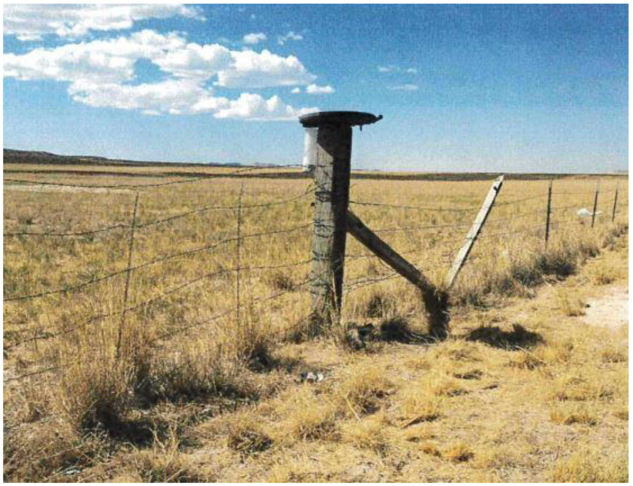
2.2. AD Sample Collection

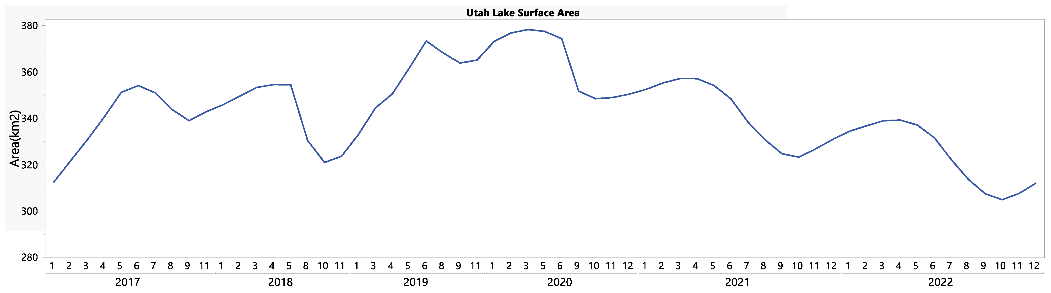
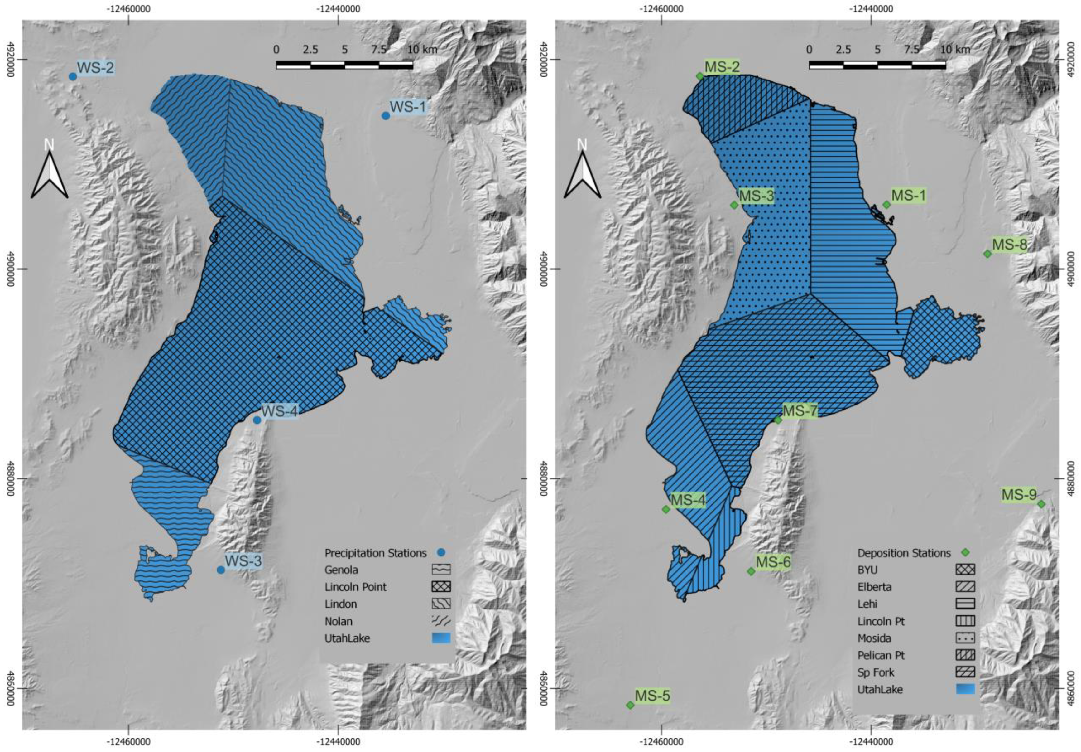
Figure 1 shows a map of the measuring station (MS) and weather station (WS) locations around the lake. The weather stations, except the Lindon station (WS-1), are located near the lake, though measuring stations MS-5 (Elberta), MS-9 (Spanish Fork), and MS-8 (BYU) are located farther from the lake in areas where prevailing winds contribute to lake AD.

Six of the nine AD stations use a sampler with a collection tube connected to a larger funnel placed approximately 2 m (7 feet) above the ground (Figure 2). These collectors are not designed to measure rainfall amounts but to collect water samples that we analyze for nutrient concentrations. The other three stations (MS-8: BYU, MS-2: Lehi Pump Station, and MS-9: Spanish Fork) are precipitation gauges located at weather stations. At these stations, we collected gauge water and analyzed it for nutrient concentrations; we did not measure rainfall volumes at any of the gages. We obtained precipitation data over the same time period from the Utah State Climate Center [27] and data on the lake area from the Central Utah Water Conservancy District (CUWCD) [28] to estimate precipitation contributions to the volume of Utah Lake.

We visually examined all samples and did not see signs of dust or solids deposition. The samplers do not generally retain even these larger particles, as the large funnel is relatively flat and any dust is easily resuspended from the surface. The nutrients in the samples are mostly from precipitation AD, with some smaller portions from settlement (dust) and dry (fine particulate matter). We attribute the loads estimated from these samples to “precipitation AD loads”, though there are minimal contributions from settlement and contact deposition processes.

We collected samples on the day following a storm event, with minor exceptions, to minimize evaporation. We visually examined the water in each sample for contaminants such as dust, bird feces, and insects. The collected samples were essentially clear, not cloudy, or otherwise dirty (contaminated), which indicates little contribution from dust or dry deposition between precipitation events. We transferred the samples from the collection tube to a capped bottle for transportation. We cleaned the collection tubes and funnels each time a sample was collected.

Chemtech-Ford Laboratories analyzed the samples for total phosphorus (TP), total inorganic nitrogen (TIN), and ortho phosphate (OP), with results reported in milligrams per liter (mg/L). Chemtech-Ford Laboratories, a TNI-accredited environmental testing laboratory, used Environmental Protection Agency (EPA) EPA 200.7 and EPA 353.2 methods for TP and TIN analysis, respectively, and method SM45000 P-E/F from Standard Methods for the Examination of Water and Wastewater (SM) for OP analysis. The TP and OP tests had detection limits of 0.007 mg/L and the TIN test had a detection limit of 0.1 mg/L. We report samples with concentrations below the detection limit as below detection limit (BDL). We obtained TP and TIN concentrations on all collected samples from 2017 to December 2022, while we only have OP measurements for samples collected after January 2019.

2.3. Lake Area Data

We obtained data for the average monthly surface area of the lake from the Central Utah Water Conservancy District (CUWCD) [28]. While these data are available on a public website, they are only stored for the three most recent months. Since the beginning of the project, we downloaded and archived these data for analysis.

Figure 3 shows the lake area over time. Beginning in October of 2016, the lake was low, with a minimal surface area. The lake volume and area rose to a peak in mid-2020, and then decreased through the end of the study period in December 2022. This graph shows that the Utah Lake surface area was quite variable over the study period.

Table 1. Surface area (km²) of Utah Lake based on a 12-month average for each year.

Lake Area (km2)	2017	2018	2019	2020	2021	2022	All
Avg	333.31	342.41	356.16	362.65	341.36	324.11	337.74
Min	312.40	321.01	333.06	348.49	323.30	304.97	312.40
Max	354.13	354.57	373.33	378.28	357.20	339.26	378.28

provides a summary of the surface area of Utah Lake for each full year of the study period. The annual average lake area ranges from 325 km² to 360 km² in 2022 and 2020, respectively, with monthly values ranging from a low of 305 km² in 2022 to a high of 380 km² in 2020. This is a range of 75 km², which represents a change of about 25%.

2.4. Load Calculation

2.4.1. Analysis Overview

We used three different methods to compute loads and loading rates of TP, TIN, and OP. All three methods compute a total load for each nutrient to the surface of the lake between sample collection dates. We integrated these data to compute total monthly and yearly loads and monthly and yearly loading rates, in both Mg/month and Mg/yr, respectively, where 1 Mg is 1000 kg.

For Method 1, we used the mean of the nutrient concentrations using data from each of the nine samplers; we then computed four different loads using these data and precipitation from each of the four weather stations combined with the monthly lake area. We then averaged these four loads to estimate the load for the event for each nutrient. For Method 2, we computed weighted averages of both nutrients and precipitation using Thiessen polygons areas. We used these weighted averages combined with the monthly lake area to compute the load. For Method 3, we used inverse distance weighting (IDW) interpolation to generate precipitation and nutrient concentration rasters for each sample date. We then computed the load for the event by multiplying each nutrient raster by its respective precipitation raster using the nominal lake area. Afterwards, we adjusted the computed load by the percent of lake area (based on the nominal area) for the sample period. We provide details on each method below.

2.4.2. Method 1

For Method 1 (M1), we computed the arithmetic mean of the nutrient concentration for each sampling event. We excluded stations where samples were not collected or analyzed. For samples with values reported as BDL, we used half of the respective nutrient detection limit. We then computed four different load values for each nutrient using precipitation measurements from each station according to Equation (1):

$$L_{M1x}=\overline{C}\ast P_x\ast A_M$$

(1)

where $P_x$ is the precipitation at each weather station, x ranges from 1 to 4 corresponding to the four weather stations, $L_{M1x}$ is the load computed using the precipitation from station x, $\overline{C}$ is the average concentration measured at the MS stations, and $A_M$ is the lake area for the month in which the event occurred. The event load was computed by averaging the loads computed using each of the four precipitation values according to Equation (2):

$$L_{M1}=\mathrm{R}\frac{1}{4}\sum _{x=1}^4{L}_{M1x}$$

(2)

where x represents the WS and $L_{M1}$ is the estimated load for the event computed using M1. The lake loading rate computed via Method 1 is the average of the results for the four different weather stations using the average nutrient concentrations for each event and the lake area at the time of the event. R is a constant for unit conversion. The original data measured $P_x$, $\overline{C}$, and $A_M$ in units of inches, mg/L, and acres, respectively, which gives units, before conversion, of $\frac{\left(\mathrm{m}\mathrm{g}\right)\left(\mathrm{i}\mathrm{n}\mathrm{c}\mathrm{h}\right)\left(\mathrm{a}\mathrm{c}\mathrm{r}\mathrm{e}\mathrm{s}\right)}{\mathrm{L}}$. To convert $L_{M1}$ to tons (i.e., 2000 lbs.), we used an R value of $1.133\times {10}^{-4}$ $\frac{\left(\mathrm{t}\mathrm{o}\mathrm{n}\mathrm{s}\right)\left(\mathrm{L}\right)}{\left(\mathrm{m}\mathrm{g}\right)\left(\mathrm{i}\mathrm{n}\mathrm{c}\mathrm{h}\right)\left(\mathrm{a}\mathrm{c}\mathrm{r}\mathrm{e}\mathrm{s}\right)}$. To convert to metric tons (${10}^3·\mathrm{k}\mathrm{g}$) or (Mg), we used an R value of 1.03 × 10⁻⁴ $\frac{\left(\mathrm{M}\mathrm{g}\right)\left(\mathrm{L}\right)}{\left(\mathrm{m}\mathrm{g}\right)\left(\mathrm{i}\mathrm{n}\mathrm{c}\mathrm{h}\right)\left(\mathrm{a}\mathrm{c}\mathrm{r}\mathrm{e}\mathrm{s}\right)}$ based on a conversion of English tons to metric tons of 0.909091 Mg/ton.

2.4.3. Method 2

For Method 2 (M2), we computed two sets of Thiessen polygons, one for the weather stations and one for the measuring stations shown in Figure 4. We used the polygon of Utah Lake available for download from the Utah Geospatial Resource Center (UGRC), which is derived from the National Hydrography Database [29], to determine the spatial extent and area of Utah Lake. We intersected the lake polygon with the Thiessen polygons to determine what percentage of the lake area was associated with each station. We then computed weighted averages for both precipitation and nutrient concentrations based on these area weights as

$$\begin{gathered} {\overline{C}}_W=\sum _{i=1}^n{W}_i{C}_i \\ {\overline{P}}_W=\sum _{j=1}^m{W}_j{P}_j \end{gathered}$$

(3)

where ${\overline{C}}_W$ is the areal weighted average concentration (mg/L), ${\overline{P}}_W$ is the areal weighted average precipitation, $W_i$ is the weight of the ith MS station, $W_j$ is the weight of the jth WS-station, and n and m are the number of MS and WS, respectively. The subscript W represents the weighted average. We computed the load to the surface of the lake for each event as

$$L_{M2}={\overline{C}}_W{\overline{P}}_W{A}_{M}R$$

(4)

where $L_{M2}$ is the load computed for the event using Method 2. To compute the monthly and annual loads, we summed or integrated the loads from each event over the subject month or year.

Table 2. Numeric summary of weights for each of the WSs (weather stations) computed using Thiessen polygons.

Measuring Station	Polygon Area (km2)	Percent Area	Weight
WS-1	118.28	32.06%	0.3206
WS-2	33.43	9.06%	0.0906
WS-3	30.63	8.31%	0.0831
WS-4	186.59	50.57%	0.5057
Total	368.93	100.00%	1.00

presents the areas, percents, and weights for each WS based on the Thiessen polygon analysis shown in Figure 4. For precipitation weighting, WS-1 and WS-4 account for over 80% of the area, with stations WS-2 and WS-3 accounting for less than 10% each. This means that the precipitation measurements from WS-4 will account for slightly over 50% of the weighted average, with WS-1 accounting for a little over 30%.

Table 3. Numeric summary of the weights for each of the MSs (measuring stations) computed using Thiessen polygons.

Measuring Station	Polygon Area (km2)	Percent Area	Weight
MS-1	79.17	21.46%	0.2146
MS-2	26.12	7.08%	0.0708
MS-3	78.69	21.33%	0.2133
MS-4	42.91	11.63%	0.1163
MS-5	0.00	0.00%	0.0000
MS-6	11.66	3.16%	0.0316
MS-7	109.46	29.67%	0.2967
MS-8	20.92	5.67%	0.0567
MS-9	0.00	0.00%	0.0000
Total	368.93	100.00%	1.0000

presents the areas, percents, and weights for each MS based on the Thiessen polygon analysis shown in Figure 4. This shows that MS-5 and MS-9 do not contribute to the weighted average nutrient concentrations, as other stations are closer to the lake. Both stations are located well away from the lake, and do not necessarily measure lake AD. Contributions to the weighted average nutrient concentration at the center of the lake are relatively evenly distributed, with MS-1, MS-3, and MS-7 each contributing between 20% and 30%. The remainder of the stations mostly contribute to the bays and northern end of the lake, but even combined with each other, contribute about 10% or less to the total.

2.4.4. Method 3

For Method 3, we computed weighted averages of the nutrient and precipitation values using inverse distance weighting (IDW) interpolation across a grid representing the surface of Utah Lake. We implemented IDW in python with a distance exponent of 2; i.e., inverse distance squared. We interpolated the data onto a 30 m × 30 m grid, then clipped both the nutrient and precipitation grids by the Utah Lake polygon. After clipping, we multiplied each nutrient raster by the corresponding precipitation raster and created a new raster that represented the load to each grid cell. We multiplied each cell by the cell areas (900 m²) and summed the value of all the cells to get the total load. We scaled the results by the ratio of the monthly average surface area of Utah Lake to the Utah Lake polygon to generate the load to the lake from the event. This can be summarized as

$$L_{M3}=\frac{A_M}{A_P}\sum \left(N_r{P}_r{A}_c\right)$$

(5)

where $N_r$ is the nutrient raster, $P_r$ is the precipitation raster, $A_c$ is the area of a cell (900 m²), $A_M$ is the monthly lake area at the time of the event, and $A_P$ is the area of the lake polygon, which is 368.933 km² (91,165.37 acres).

Method 3 uses the precipitation and nutrient concentration computed for each cell, which vary considerably for each event. Figure 5 shows the precipitation (top) and TP nutrient (bottom) rasters for three different events. In this figure the nutrient color scale remains constant with a range from 0 to 2.5 mg/L, while the precipitation scale varies from 0 to 30 mm, 0 to 1 mm, and 0 to 5 mm from the left to the right, respectively, to better show variation in precipitation for each event. The left image is the highest precipitation (0–30 mm), the middle the lowest (0–1 mm), and the right is an in-between amount (0–5 mm). This set of events includes two events with high nutrient values, 8 June 2020 (left) and 23 May 2021 (center), and one event with very low nutrient values on 7 November 2022 (right). Associated with these nutrient events are a high precipitation event (left), a very low event (center), and an average event (right). The associated loads are 10.5 Mg, 0.2 Mg, and 3.0 Mg from left to right, respectively. This shows that a high nutrient concentration, such as the center event (23 May 2021), can result in a low load if associated with a small rainfall, while a low nutrient event such as the right event (7 November 2022) can result in a meaningful load if precipitation is large enough.

3. Results

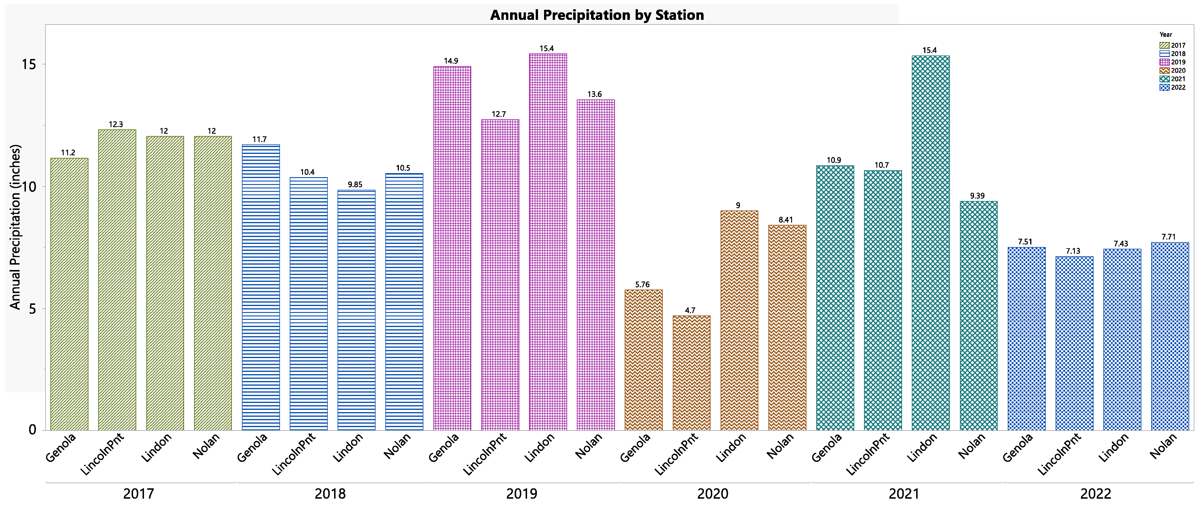
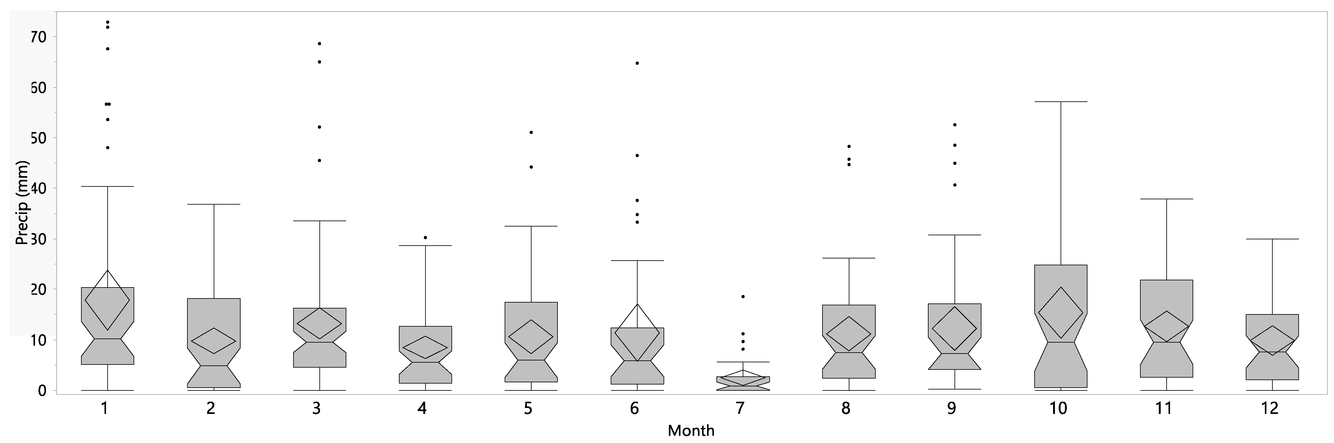
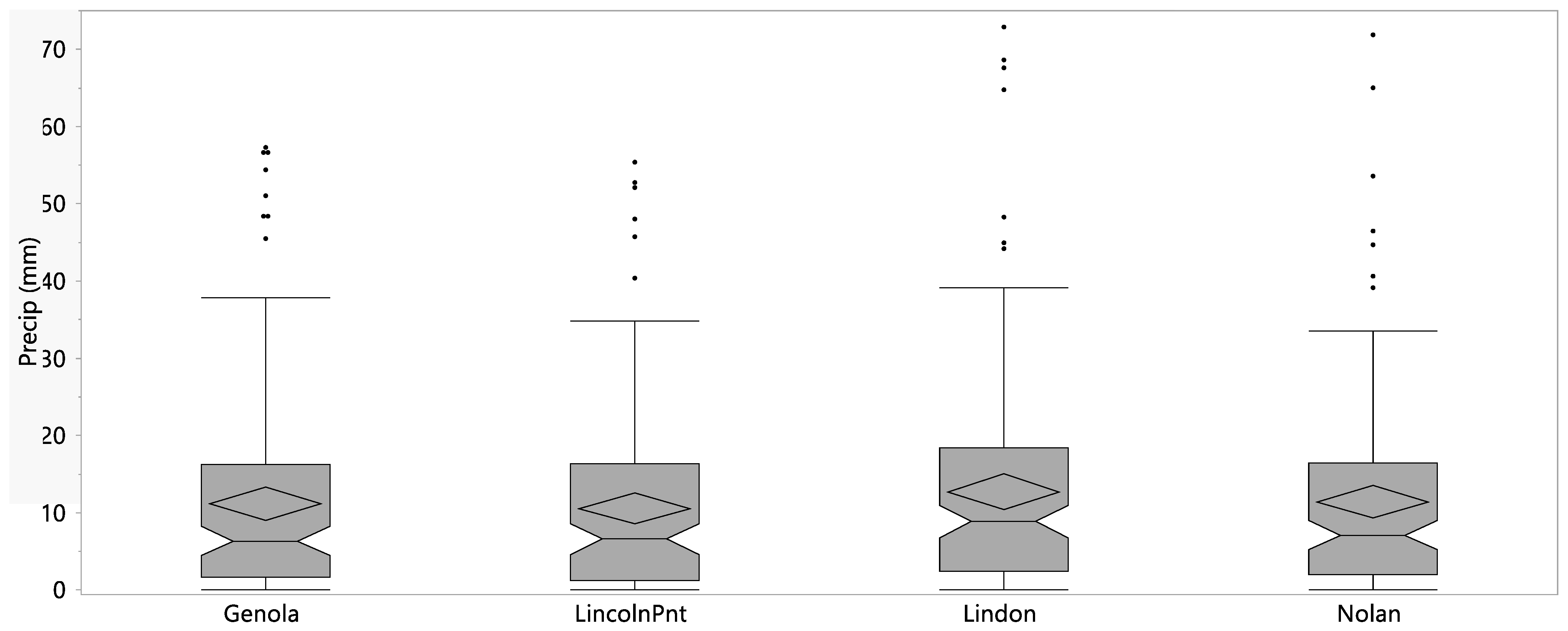
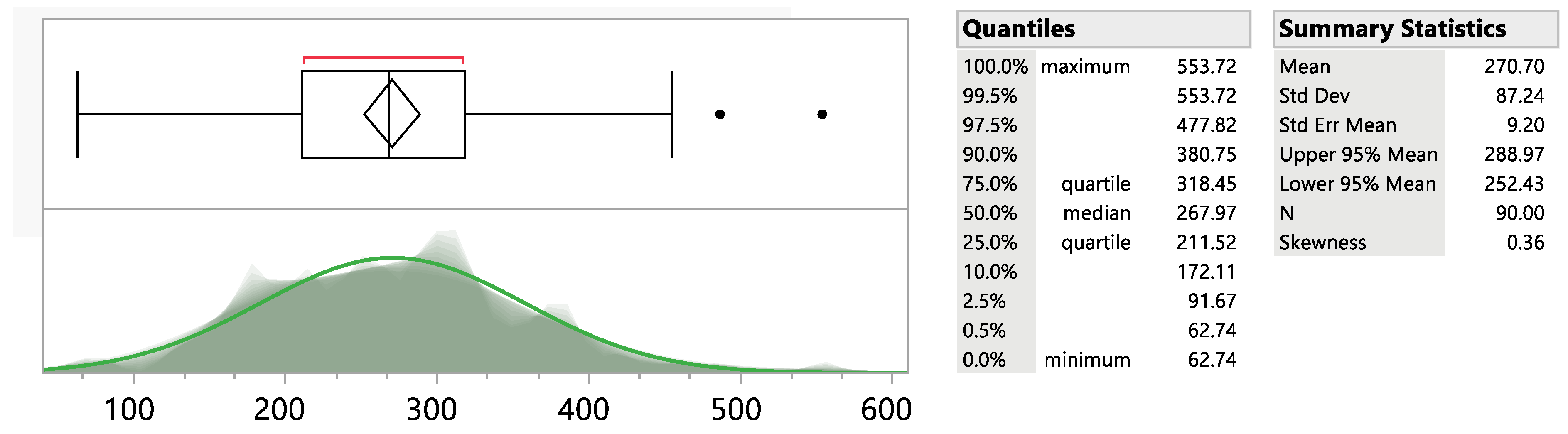
3.1. Precipitation Data

We obtained daily precipitation data from the Utah Climate Center, managed by Utah State University, for four weather stations around the lake, as shown in Figure 1 [27]. We summed the total precipitation measured at each station between sample dates to quantify the total precipitation amount measured at each station and associate it with each nutrient measurement over the sample period.

Figure 6 shows the annual total precipitation for each station over the study period: 2016 only includes data from October, November, and December. The data show that the first three years (2017–2019) were wetter than the last three (2020–2022), though 2021 was somewhat higher. These data show that the stations’ measurements are similar in any given year, though in 2021, WS-1 (Lindon) had significantly higher precipitation than the other stations.

Figure 7 shows a distribution of the monthly precipitation for each month. This figure includes data from all four stations, so for any given month and year, there are four stations, which over a 6-year study period results in between 24 and 28 measurements for each month. The data show that the heaviest precipitation comes from October through March. The winter months of November, December, and January have mean values similar to their median value, while the October data are skewed, with the median lower than the mean. This indicates that the October distribution is governed by a few larger events. July is the driest month, and April through June are slightly wetter. August and September have mean and median values similar to November and December, but not as high as January and February.

Figure 8 presents the precipitation distribution by station. The boxplots show that the data are similar among the stations, with Lindon having a slightly higher average and median precipitation than the other stations. Median and mean values for the other three stations are similar to each other. At the 75th percentile, Genola and Lindon are similar, and Lincon Point and Nolan are similar. All stations have a few data points beyond the 75th percentile, with Nolan and Lincon Point having the highest values.

Table 4. A pairwise ordered difference report for precipitation events at the four water stations.

Site	Site	Diff. from Mean	Std. Err. Diff.	Lower CL	Upper CL	p-Value
WS-1 (Lindon)	WS-4 (Lincoln Pnt)	2.163	1.543	−0.868	5.195	0.162
WS-1 (Lindon)	WS-3 (Genola)	1.540	1.543	−1.492	4.571	0.319
WS-1 (Lindon)	WS-2 (Nolan)	1.308	1.543	−1.724	4.340	0.397
WS-2 (Nolan)	WS-4 (Lincoln Pnt)	0.855	1.543	−2.176	3.887	0.580
WS-3 (Genola)	WS-4 (Lincoln Pnt)	0.623	1.543	−2.408	3.655	0.686
WS-2 (Nolan)	WS-3 (Genola)	0.232	1.543	−2.800	3.264	0.881

presents a pairwise ordered difference report comparing the precipitation data by station using Student’s t-test. At a significance level of 5% (α = 0.05), the data means for the different stations are not significantly different, with the lowest p-value being 0.162, well above 0.05. This means that statistically, we can assume the data from all the stations are likely from the same distribution over the 6-year study period.

Figure 9 shows a graph of the analysis of means (ANOM) analysis, which presents the same conclusions as the Student’s t-test: statistically, we cannot say that the mean values from the four stations are different at the 95% level, and any difference can be explained by variability in the data.

We obtained precipitation data from the Utah Climate Center at Utah State University [27]. The average annual precipitation over the study period was 265 mm, which is in the 47th quantile, slightly below the 90-year average, with the highest and lowest annual precipitation of 359.5 mm and 177.0 mm in 2019 and 2020, which represent the 84th and 14th quantiles of the 90-year record at Lehi, respectively (Figure 10). At the weather stations, annual precipitation ranged from 119 mm/yr to 392 mm/yr measured at WS-4 (Lincoln Point) in 2020 and WS-1 (Lindon) in 2019, respectively, with the high measurement being 3.19 times the lower. These values are below the 5th and above the 90th quantile, respectively (Figure 10).

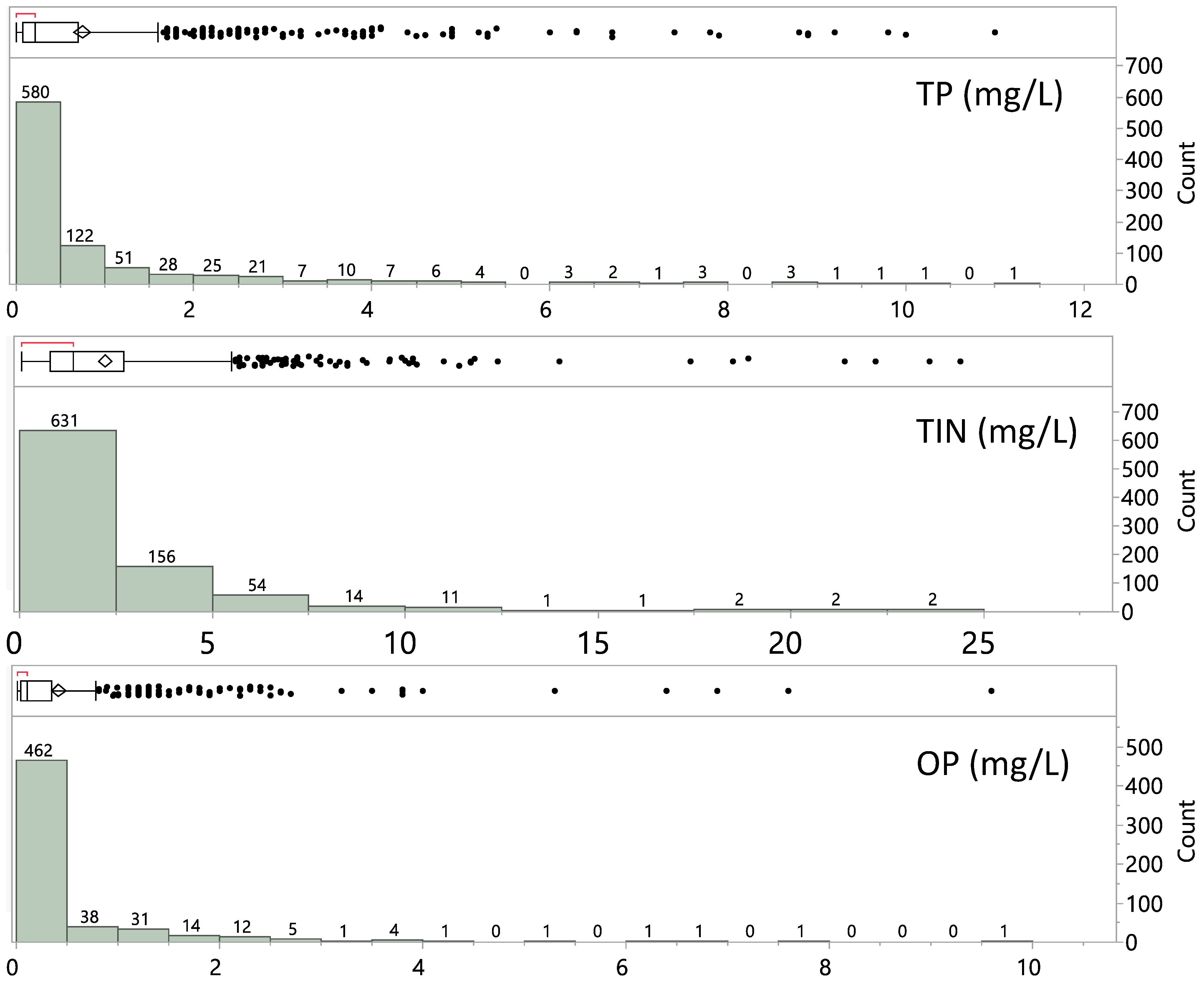
3.2. Precipitation Nutrient Sample Data

Storms in Utah Valley commonly do not cover the entirety of Utah Lake or the surrounding city owing to the effects of the surrounding mountains and high-elevation desert climate. Consequently, some precipitation events are not recorded at all the measuring stations. This is not an error in the collection or recording process. We only collected samples if there was water in the sampler. For TIN and TP, we collected between 88 and 108 samples depending on the station (

Table 5. Statistical summary of nutrient concentration data.

Constituent	Station	Num. of Samples	Mean (mg/L)	Median (mg/L)	Max. (mg/L)	Skew
Phosphorous (TP)	MS-1	97	0.65	0.26	8.90	4.85
	MS-2	108	0.99	0.32	11.00	3.46
	MS-3	92	0.94	0.25	7.80	2.59
	MS-4	88	1.13	0.60	5.20	1.54
	MS-5	98	0.63	0.31	4.90	3.31
	MS-6	104	0.90	0.28	10.00	3.52
	MS-7	98	1.18	0.41	8.90	2.57
	MS-8	94	0.13	0.06	1.20	3.39
	MS-9	98	0.18	0.07	2.70	5.03
Nitrogen (TIN)	MS-1	97	2.70	2.10	22.20	3.98
	MS-2	107	2.23	1.80	11.70	1.99
	MS-3	95	2.77	1.50	18.50	2.57
	MS-4	88	2.68	1.90	10.30	1.45
	MS-5	98	1.80	1.40	8.50	1.77
	MS-6	103	1.58	1.00	11.80	2.72
	MS-7	102	3.09	1.46	24.40	3.05
	MS-8	88	1.77	1.30	9.59	2.15
	MS-9	96	1.36	1.10	6.70	2.32
Ortho Phosphate (OP)	MS-1	65	0.30	0.12	2.10	2.70
	MS-2	69	0.52	0.16	4.00	2.44
	MS-3	59	0.51	0.14	3.80	2.50
	MS-4	63	0.78	0.32	7.60	3.66
	MS-5	68	0.32	0.14	3.20	3.59
	MS-6	71	0.22	0.10	1.70	2.59
	MS-7	70	0.87	0.21	9.60	3.39
	MS-8	49	0.03	0.02	0.11	1.31
	MS-9	59	0.06	0.04	0.40	2.74

), while we collected between 49 and 71 samples for OP depending on the station (Table 5).

Table 5 provides a statistical summary of the number, mean, median, maximum, and skew of measured concentrations data for each measuring station and constituent. The minimum value for each station is 0.00 mg/L and is not shown. The raw concentration data are available in the electronic supplement to this article.

The median concentrations are consistently lower than the mean concentration and have relatively large positive skew values, which shows that these data are right skewed, with significantly more samples associated with low concentration values. Figure 11 shows the distributions of all three analytes: TP, TIN, and OP. All the analytes have samples with relatively large values, though the load contributed by these large values is dependent on the associated precipitation event, as the load is computed as a function of both the precipitation amount and the analyte concentration.

Figure 12 shows TP concentration distributions by measuring station (we do not show the distributions for TIN and OP). The boxes represent the 25th and 75th percentiles, with the notch and line at the 50th percentile (i.e., median), the diamond indicates the mean values at the center with 95% confidence intervals at the points, and the whiskers indicate 1.5 times the interquartile range (IQR). Outlier values greater than 1.5 times the IQR are shown as dots. These plots exclude outliers greater than 5 mg/L for visualization purposes, though all values were used to compute the statistics. Figure 12 shows that the measured TP concentrations at the MS-8 (BYU) and MS-9 (Spanish Fork) stations are lower than at the other stations. These two stations are farther away from the lake and at higher elevations than the closer stations. The medians for the other stations are similar, with a higher mean for stations on the west side of the lake and Lincoln Point.

We used two different statistical tests to compare the mean TP concentrations (

Table 6. Statistical comparison of mean TP measurements pairwise by measuring station with an alpha value of 0.05.

Site	Name	Mean	Student’s t			Tukey–Kramer HSD
MS-7	Lincoln Pt	1.180	A			A
MS-4	Mosida	1.129	A			A
MS-2	Lehi	0.986	A	B		A
MS-3	Pelican Pt	0.939	A	B		A
MS-6	Genola	0.904	A	B		A
MS-1	Orem	0.654		B		A	B
MS-5	Elberta	0.628		B		A	B
MS-9	Spanish Fork	0.181			C		B
MS-8	BYU	0.126			C		B

). We present the analysis of TP, though the other nutrients are similar. We performed a pairwise comparison using Tukey–Kramer HSD and Student’s t-test with an alpha value of 0.05 in the software program JMP 16.1. This is not a comparison of loads, as loads are a function of both concentration and precipitation. Table 6 is a comparison of the mean nutrient values measured at each location to analyze precipitation concentration similarities and differences.

Table 6 is a connected letter report on the pairwise comparison from both statistical tests. If two sites are connected by a letter, then there is no statistical evidence of difference at the 95% confidence level. For instance, the first five rows for stations MS-7, MS-4, MS-2, MS-3, and MS-6 all have a letter A in the Student’s t test column. That means they are not statistically significantly different from each other. Three stations in group A also have a letter B, meaning they are not statistically significantly different from the stations on rows 3–7. The stations listed on rows 1 and 2 (MS-7 and MS-4) are statistically significantly different from the stations listed on rows 6 and 7 (MS-9 and MS-8), since they are part of group A but not group B.

The two tests provide different results. The Student’s t-test divides the stations into three groups, with MS-9 (Spanish Fork) and MS-8 (BYU), the sites with the lowest means, in an independent group C. The five sites with the highest means are in group A, while the five sites, starting with MS-2 (Lehi), in the middle belong to group B. MS-2 (Lehi), MS-3 (Pelican Pt), and MS-6 (Genola) are statistically similar to some sites in both groups A and B. The Tukey–Kramer test only classifies the stations into two groups, with the top seven sites in group A and the bottom four sites in group B. In this test, the MS-8 (BYU) and MS-9 (Spanish Fork) sites are not significantly different from Orem and Elberta, while the Student’s t-test indicated they are different. Both tests indicate that the bottom four stations, Orem, Elberta, Spanish Fork, and BYU are different from the top two stations.

Figure 13 shows an analysis of means (ANOM) plot [30], generated using JMP 16.1. This plot shows that MS-8 (BYU) and MS-9 (Spanish Fork) are below the group decision levels, while MS-7 (Lincoln Point) and MS-4 (Mosida) are above. This reinforces the analysis from the Student’s t-test and the Tukey–Kramer HSD test. The electronic data supplement contains a full report on these analyses, including ordered pairwise means analysis for both the Student’s t and Tukey–Kramer analysis.

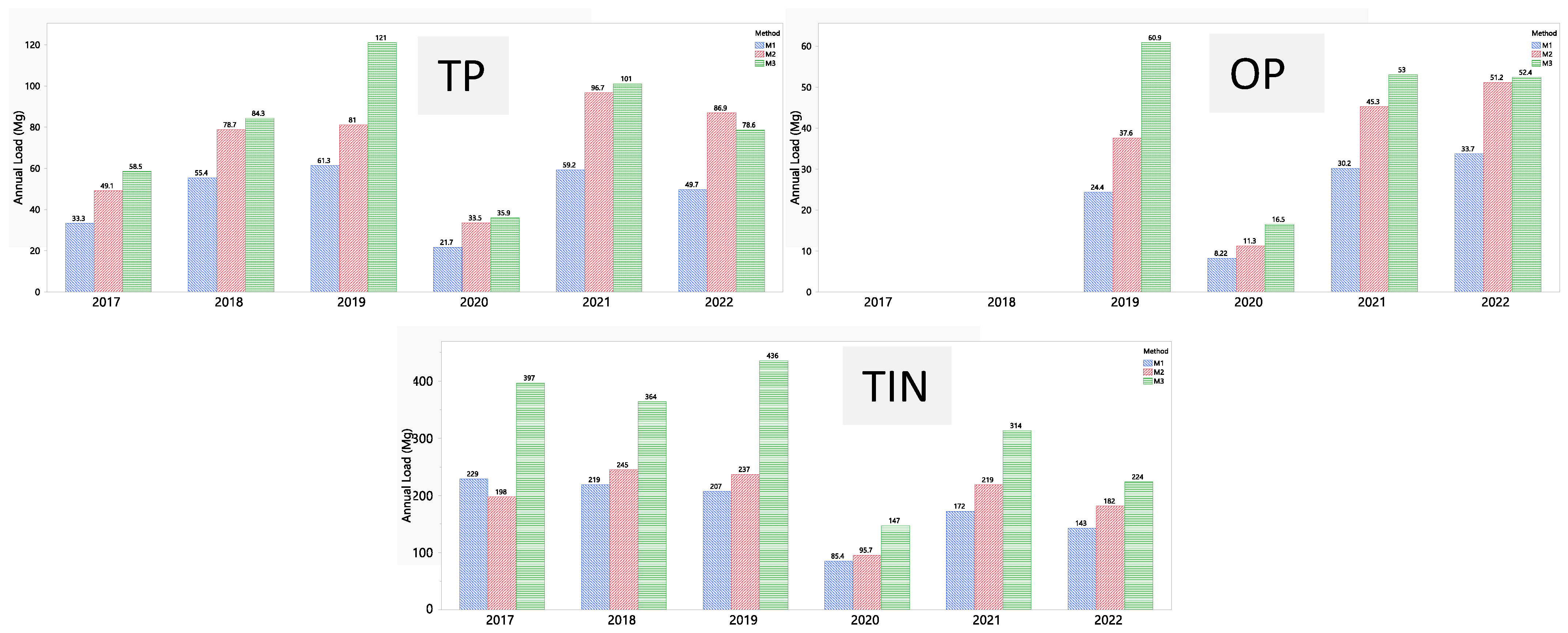
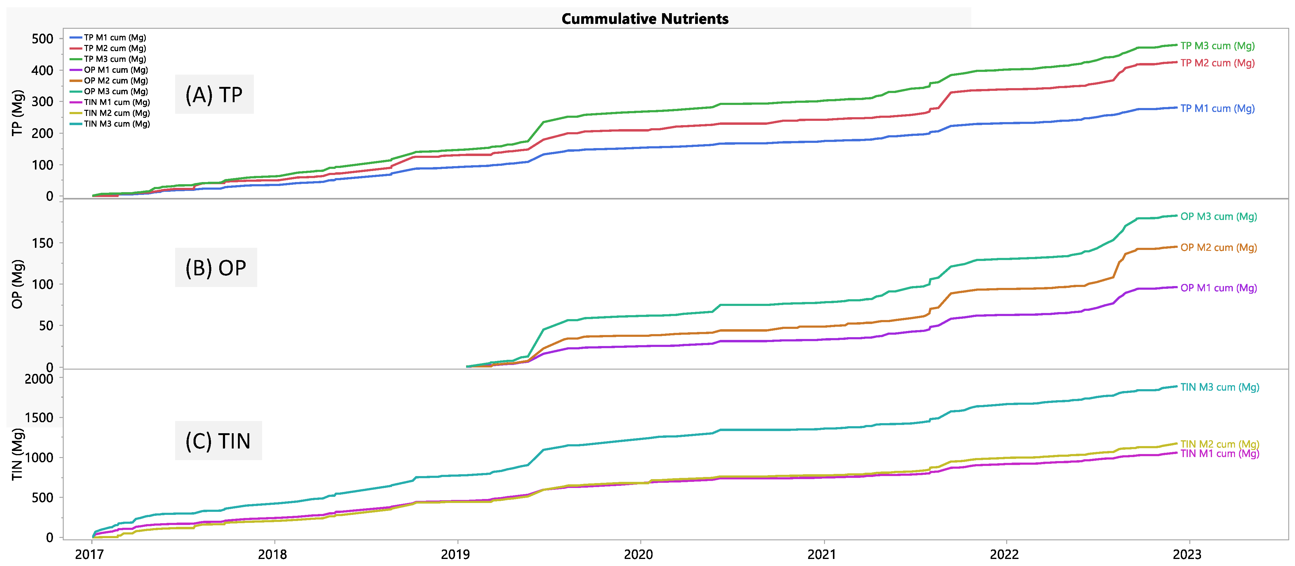
3.3. Total Nutrient Loads

Table 7. Summary of annual year loads for each method and their average for each year and the averages over the 6-year study period. It also includes the percent difference of each 6-year average from the mean value over the 6-year period.

Nutrient	Method	2017 (Mg/yr)	2018 (Mg/yr)	2019 (Mg/yr)	2020 (Mg/yr)	2021 (Mg/yr)	2022 (Mg/yr)	6-Year Average (Mg/yr)	Diff. from Average
TP	M1	33.26	55.40	61.33	21.68	59.18	49.68	46.76	−29%
	M2	49.06	78.73	81.03	33.51	96.66	86.85	70.97	8%
	M3	58.47	84.26	120.96	35.93	101.05	78.63	79.88	21%
	Average	46.93	72.80	87.77	30.37	85.63	71.72	65.87	0%
TIN	M1	229.09	218.96	207.20	85.38	172.49	142.84	175.99	−23%
	M2	197.58	244.81	237.01	95.73	218.63	181.53	195.88	−14%
	M3	396.89	364.05	435.89	147.37	313.51	223.73	313.57	37%
	Average	274.52	275.94	293.37	109.49	234.88	182.70	228.48	0%
OP	M1			24.36	8.22	30.21	33.72	24.13	−32%
	M2			37.62	11.25	45.25	51.17	36.32	3%
	M3			60.87	16.51	53.04	52.41	45.71	29%
	Average			40.95	11.99	42.83	45.77	35.39	0%

summarizes the annual nutrient loads (Mg/yr) for each year for each analysis method. It also presents an average of the three methods’ load for each year, and an average over the 6-year study period for both each of the three methods and the average of the three methods. The right column is the difference in the average for each method over the 6-year study period compared with the average of all the methods over the study period.

Annual average TP loads range from 30.37 to 87.77 Mg/yr for 2020 and 2019, respectively. The largest estimated load was 120.96 Mg/yr, estimated using M3 in 2019, with the lowest load of 21.68 Mg/yr being estimated using M1 in 2020. The 6-year averages range from 46.76 Mg/yr to 79.88 Mg/yr for M1 and M3, respectively, with an average value of 65.87 Mg/yr. The 6-year average estimates ranged from −29% to 21% for M1 and M3, respectively, with M2 being 8% different from the average. The behavior for TIN and OP is similar, with M1 estimating the lowest annual loads and M3 the highest. Both TIN and OP ranges, in percentage terms, are larger than that for TP.

Figure 14 summarizes the annual loads for all three nutrients, TP, TIN, and OP in Mg/yr for each of the three methods. These graphs show that 2020 had the lowest loads, with higher loads in the remaining years. All three methods estimated similar loads for TP and OP except for 2019, when M3 was significantly higher. M3 consistently estimated higher loads for TIN in all years.

Figure 15 presents cumulative loads (Mg) for each of the three nutrients and methods over the 6-year period (4 years for OP). For all three nutrients, M3 estimates the highest load, with M1 estimating the lowest. For TP, the M3 and M2 methods are similar, with M1 estimating lower, while for OP, the methods are about evenly separated. For TIN, the M2 and M1 methods are similar, with M3 being significantly higher.

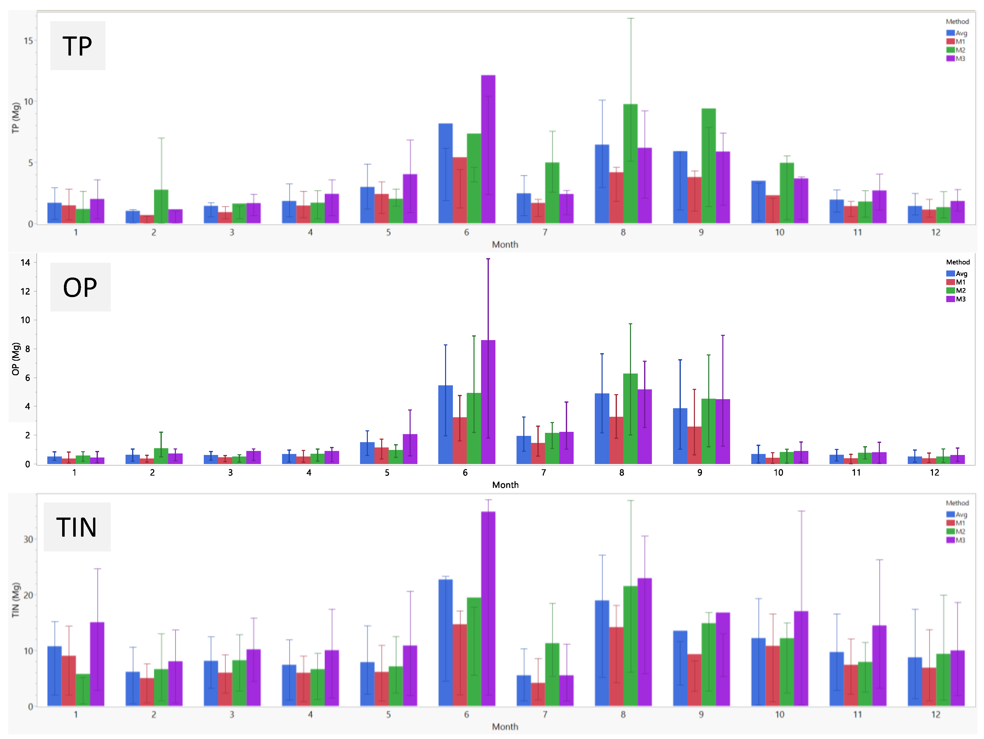
3.4. Average Monthly Nutrient Loads

Figure 16 and

Table 8. Summary of monthly loading rates for each nutrient and method in Mg/month averaged over the 6-year study period.

Nutrient	Method	Monthly Average Load (Mg/month)
		1	2	3	4	5	6	7	8	9	10	11	12
TP	M1	2.69	1.68	2.89	3.39	5.19	7.21	1.95	8.36	6.30	3.82	2.35	0.93
	M2	1.76	3.21	4.31	3.65	4.01	8.57	4.15	17.90	12.53	7.42	2.37	1.10
	M3	3.64	3.05	5.22	5.62	8.71	16.17	3.21	12.36	9.79	6.12	4.48	1.52
	Avg	2.70	2.65	4.14	4.22	5.97	10.65	3.10	12.87	9.54	5.79	3.07	1.18
TIN	M1	18.05	12.55	18.97	13.94	13.28	19.59	4.84	28.32	13.97	14.41	12.33	5.74
	M2	9.60	7.72	21.93	14.33	14.23	22.73	9.40	39.48	19.82	18.28	10.57	7.80
	M3	30.09	21.44	32.20	23.40	23.53	46.49	7.36	45.90	25.18	25.55	24.11	8.32
	Avg	19.25	13.90	24.37	17.22	17.01	29.60	7.20	37.90	19.66	19.41	15.67	7.29
OP	M1	2.27	1.5	5.41	3.62	9.12	19.45	5.8	26.1	15.5	3.43	2.32	1.97
	M2	2.34	3.26	6.08	4.21	6.75	24.65	8.59	50.17	27.12	5.74	3.86	2.52
	M3	2.66	2.87	10.72	6.27	16.46	51.62	8.86	41.39	26.98	7.11	4.87	3.04
	Avg	2.42	2.54	7.40	4.70	10.78	31.91	7.75	39.22	23.20	5.43	3.68	2.51

summarize the monthly loads (Mg/month) averaged over the study period. This includes loads for each of the three nutrients, each of the three analysis methods, and an average of the three analysis methods. July and December have the lowest average loading rates, while the highest average loading rates are in June or August. For both TP and OP, loading rates are relatively low and constant from November through May, with a slight increase in May. Larger loads occur in June, then August through October. TIN loading rates are relatively constant, except for higher loads in June and August and lower rates in July and December.

3.5. Monthly Loading Rates

To be useful for modeling and planning, we computed the monthly loading rates as a percentage of the annual loading rate shown in

Table 9. Monthly loading rates as percent of annual rates averaged over the study period.

Nutrient	Method	Monthly Percentage Load of Annual Load (%)
		1	2	3	4	5	6	7	8	9	10	11	12
TP	M1	6%	4%	6%	7%	11%	15%	4%	18%	13%	8%	5%	2%
	M2	2%	5%	6%	5%	6%	12%	6%	25%	18%	10%	3%	2%
	M3	5%	4%	7%	7%	11%	20%	4%	15%	12%	8%	6%	2%
	Avg.	4%	4%	6%	6%	9%	16%	5%	20%	14%	9%	5%	2%
TIN	M1	10%	7%	11%	8%	8%	11%	3%	16%	8%	8%	7%	3%
	M2	5%	4%	11%	7%	7%	12%	5%	20%	10%	9%	5%	4%
	M3	10%	7%	10%	7%	8%	15%	2%	15%	8%	8%	8%	3%
	Avg.	8%	6%	11%	8%	7%	13%	3%	17%	9%	8%	7%	3%
OP	M1	2%	2%	6%	4%	9%	20%	6%	27%	16%	4%	2%	2%
	M2	2%	2%	4%	3%	5%	17%	6%	35%	19%	4%	3%	2%
	M3	1%	2%	6%	3%	9%	28%	5%	23%	15%	4%	3%	2%
	Avg.	2%	2%	5%	3%	8%	23%	5%	28%	16%	4%	3%	2%

. These percentage rates are based on the average monthly loading data from Table 8.

Table 9 shows that monthly loading rates vary depending on the nutrient. For example, the majority of TP loading occurs in May, June, August, September, and October, with values of only about 5%/month occurring in the remainder of the year. TIN AD is more evenly distributed, with monthly rates from 6% to 11% per month, except for July (3%), June (13%), and August (17%). OP AD monthly rates have distributions similar to TP rates. In general, M3 predicts higher summer rates (except for July) than the other methods. This is because of episodic large precipitation events that can weight the data towards bigger loads.

4. Discussion

We documented AD from precipitation events to Utah Lake over a 6-year period using measured nutrient concentrations in more than 850 samples taken at nine locations around the lake and showed that these loads are a substantial contribution to the Utah Lake nutrient budget. To estimate loads, we combined lake area, nutrient concentrations, and precipitation measurements from four different weather stations around the lake using three different methods. The estimated nutrient loads calculated through these methods exhibited large variations over the study period because of variations in nutrient concentrations, larger variations in precipitation amounts, and, to some extent, variations in lake surface area. Measured concentrations and precipitation amounts were variable both in time and in space, with data measured on the same day showing large differences across measuring locations. We used three different methods and found that M1 (average values) consistently estimated the lowest load, M2 (Thiessen polygons) provided a middle estimate, and M3 (IDW) generated the highest estimate.

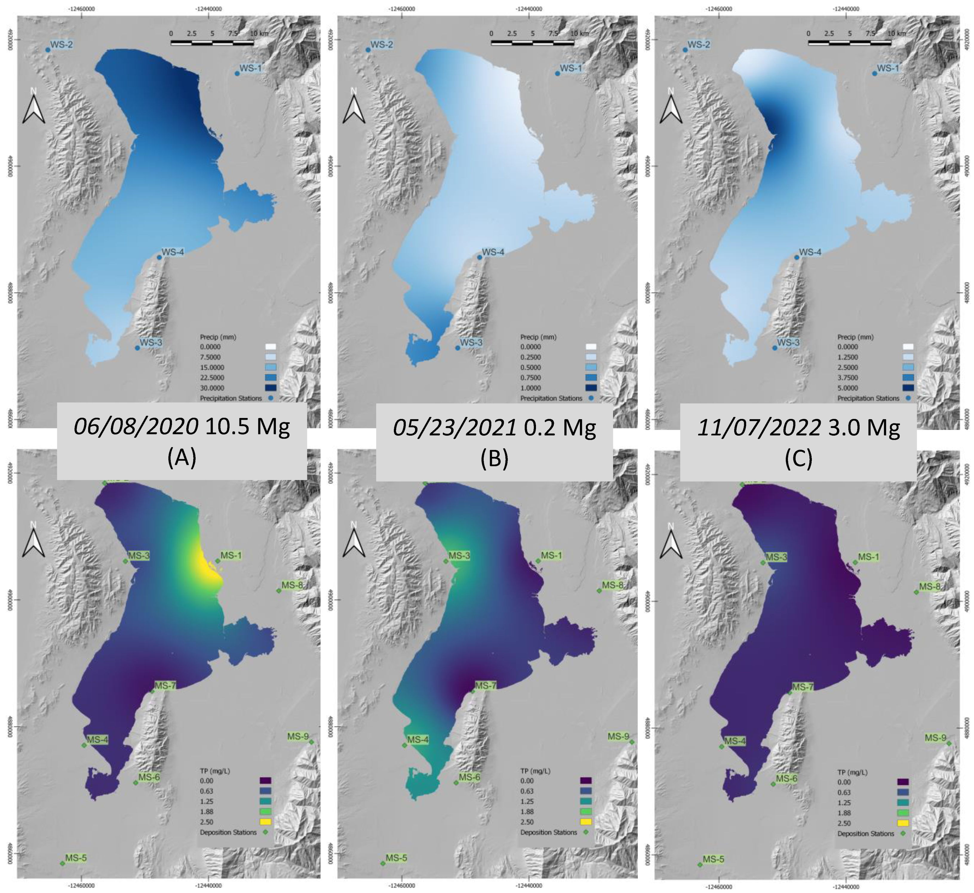
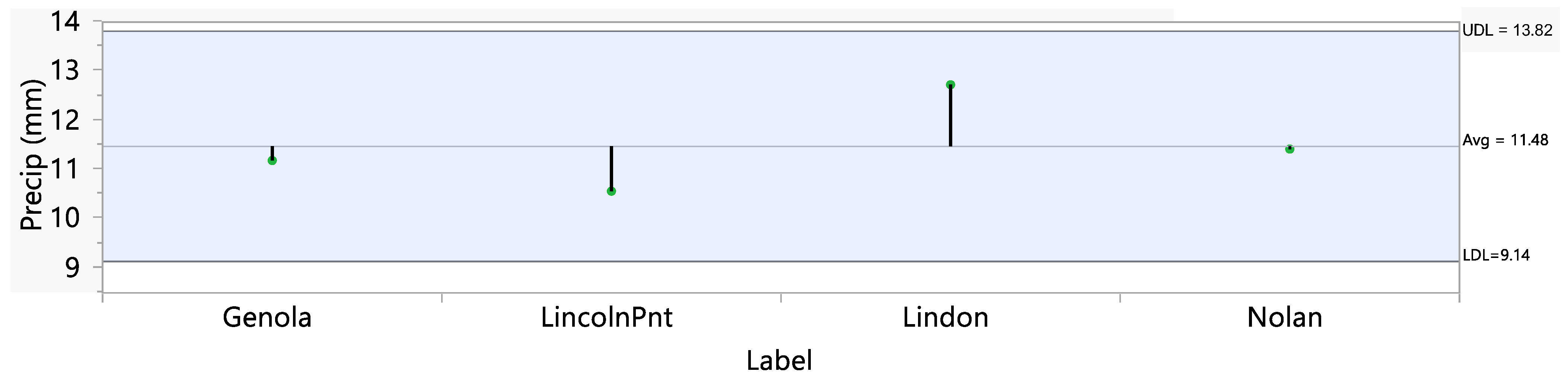
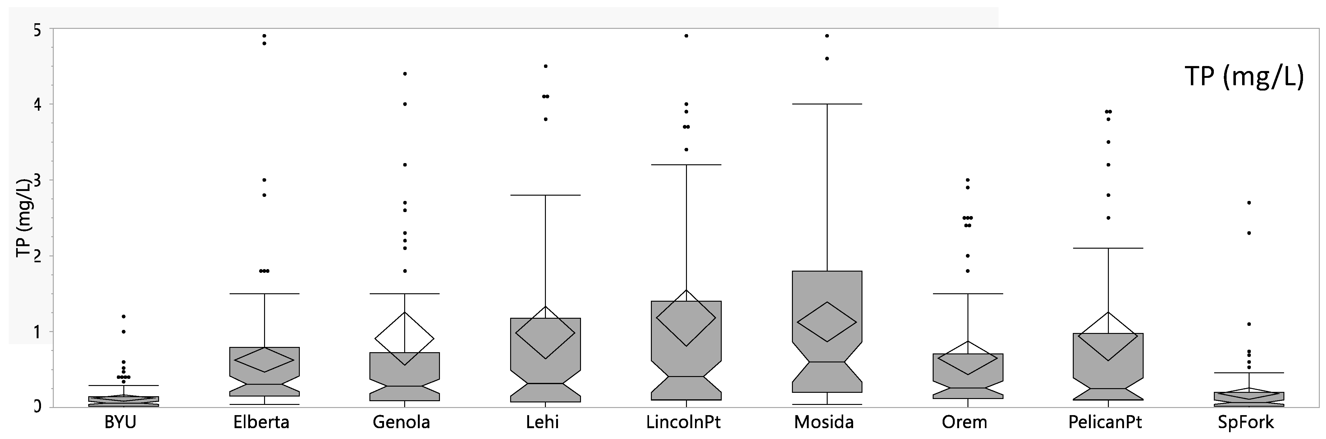
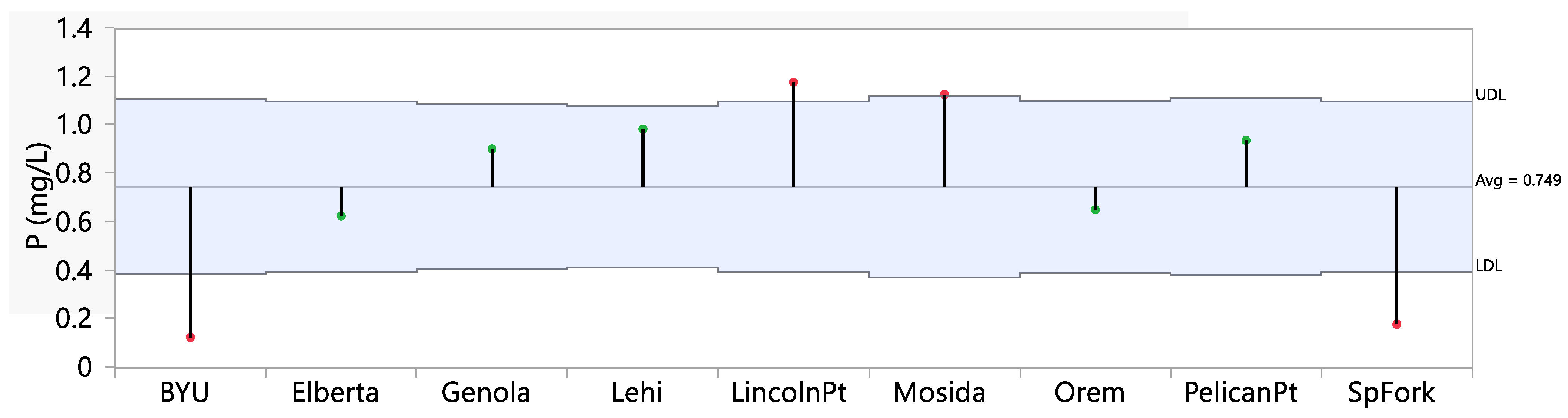
4.1. Spatial and Temporal Variation

Our data support the intuition that precipitation-related AD nutrient loads vary spatially across the lake surface due to differing nutrient concentrations and precipitation amounts measured at different locations. Because of this spatial variation, data from a single station are insufficient to estimate total loads to the lake, and data from multiple locations surrounding the lake provide a more complete estimate of AD. We hold that the more comprehensive IDW interpolation method used in M3, which combines results from multiple stations, is more accurate than the simple average (M1) or Thiessen polygon method (M2). The Thiessen method excludes some data because the polygons do not intersect the lake surface. These measurements are included in M3, though at low weights because of their distance. The simple average (M1) weights all samples equally but ignores the spatial proximity of the samples (Figure 5).

While the average precipitation over the 6-year study period was similar to the 90-year measured average from 1904 to 2003, the precipitation in the highest year was at the ~85th percentile, which gives an exceedance probability of ~0.15. This means that we would expect, on average, for this level of precipitation to be exceeded once every 6.7 years, often called a return period. The precipitation in the lowest year was at the 14th percentile, which gives a return period of slightly over 7 years. Loads are only somewhat correlated with rainfall, with coefficients of determination (R²) between precipitation and TP, TIN, and OP of 0.22, 0.40, and 0.15, respectively. While higher rainfall results do result in larger loads from precipitation AD, concentration and lake area play a significant role. Lake areas varied by 25%, and nutrient concentrations were significantly skewed, dominated by lower values.

4.2. Relation to Previous Studies

Two previous studies used an orthogonal method to measure AD to Utah Lake [10,11]. The second study modified and verified some of the field methods used in the first study [10]. These studies overlap in time with our study, though their duration is shorter. Unlike our field measurement methods, they captured and measured total nutrient deposition, which included all categories defined for this study: settlement, contact, and precipitation. They measured areal loading rates in mass/area/time, while we measured concentration. They collected data weekly, and their samplers consisted of buckets which contained distilled water. These buckets captured contact AD because of the water, settlement as dust, and precipitation. They computed the mass of each nutrient by measuring both the nutrient concentrations and water volume in the sampler. Using the measured mass and the sampler area, they computed the areal deposition rate in mass/area/week at each sampler location. They then spatially interpolated these data to compute lake AD. These studies estimate higher AD loads than our estimates, as they include both contact and settlement AD in addition to precipitation AD, which is the only process we measured.

For 2019 and 2020, Barrus et al. [10] estimated 238 and 121 Mg/yr (262 and 133 tons/yr) of TP and 956 and 438 Mg/yr (1052 and 482 tons/yr) of DIN, respectively. They used the description dissolved inorganic nitrogen (DIN) values rather than TIN, which we use. This compares to our estimates of 120.96 and 35.93 Mg/yr of TP and 435.89 and 147.37 Mg/yr of TIN for 2019 and 2020, respectively. This comparison is summarized in

Table 10. Comparison of estimates of total AD in the literature to our estimates of AD from precipitation.

Nutrient	TP [Lit.] (Mg/yr)	TP [Ours] (Mg/yr)	∆TP (Mg/yr)	DIN [Lit.] (Mg/yr)	TIN [Ours] (Mg/yr)	∆TIN (Mg/yr)
2019	238	121	117	956	436	520
2020	121	36	85	438	147	291

, which includes the difference between our values and those from the previous study as ∆TP and ∆TIN in Mg/yr.

The differences between our estimates and estimates from the previous study (Table 10) can be attributed to the nutrient load from dry deposition, which includes both contact deposition and settlement of dust. These data show that dry deposition of TP is about equal to precipitation deposition in a wet year (2019) and about three times higher in a dry year (2020). Ratios for TIN from dry and precipitation processes are about the same in both years, with about twice as much TIN AD from dry deposition as from precipitation AD.

We attribute the large fraction of dry nutrient AD to weather patterns, such as inversions, that trap particulate matter in the valley. Kuprov et al. [31] noted that Utah Valley, the location of Utah Lake, is a non-attainment area for PM₁₀ and PM_2.5, which means that particulate levels are high. Recorded data show that PM_2.5 levels averaged across 18 air quality monitors throughout the Wasatch Front (which represents the urban area where Utah Lake is located) from 2004 to 2015 were between 40 and 50 µg/m³ for the 98th percentile, while the 98th percentile for PM₁₀ averaged about 10 µg/m³ over the same time period [32]. For TIN, dry loads are higher, as TIN deposition includes nitrogen gas compounds which dissolve in the water on contact, making dry AD even more prevelent. The high particulate measurements support attributing the large difference between the previous study and our data to dry AD, as small particulate and gaseous loads are particularly large in the atmosphere above Utah Lake and readily deposited through contact with a wet surface.

4.3. Implications for Lake Management

Based on the spatial and temporal variation in nutrient concentrations, the impact of variable precipitation amounts, and comparison with previous data, we hold that the annual precipitation AD loads from 2019 estimated using M3 are the most accurate and should be used. These 2019 loads are 21%, 37%, and 29% larger than the loads averaged over the entire study period and the three methods for TP, TIN, and OP, respectively. The lake area was higher during 2019 and represents the reservoir managed under normal to high water conditions, rather than the lower levels seen recently because of drought. During other years in the study, the lake area was lower. Using the 2019 measured values for precipitation AD in management studies addresses uncertainty in the data caused by large natural variations. While we do not have sufficient data to quantify AD loads over time, the lake levels in 2019 more closely resemble normal conditions. Managers and others can use these values and adjust, based on lake levels or precipitation, if required.

Using these assumptions, our best estimates of annual precipitation AD loads to Utah Lake based on M3 in 2019 for TP, OP, and TIN are 120.96 Mg/yr (132.97 tons/yr), 60.87 Mg/yr (67.1 tons/yr), and 435 Mg/yr (479.5 tons/yr), respectively (Table 4). This compares to the 6-year average loads over the study period of 65.87, 228.48, and 35.39 Mg/yr, for TP, TIN, OP, respectively (Table 4). We recommend using the monthly load percentage rates (Table 9) to compute monthly loads based on these annual values. These recommended loads should be used as a “best estimate” for precipitation AD nutrient loads to Utah Lake, while loads scaled to represent longer return periods should be used for prediction models, especially over longer planning periods where we would expect these loads to be exceeded regularly. We did not compute return periods for nutrient loads due to the very short analysis period, but based on the precipitation data, we would expect return periods of approximately 10 years or less.

The Utah Lake Science Panel estimated that dust contributes about 27 Mg/yr (30 tons/yr) of TP [24,26]. Estimates of the contributions of dust AD from previous studies [26] and the Utah Lake Science Panel, combined with our data, suggest that AD from dust is about 10% to 15% of the total, and that from precipitation AD is about 42% of the total using data from 2020. In 2019, precipitation AD was only 25% of the total, even though this was a wet year (Figure 6). This could possibly be due to the storms not allowing strong inversions with high particulate counts to form, though we have no data to support this hypothesis. These percentages are computed as the percentage of the total nutrient AD to Utah Lake from Barrus et al. [10], shown in Table 10.

While this study focused on precipitation AD, AD from other sources, such as dust and dry deposition provide a significant nutrient load to the lake. For any nutrient budget models, managers should use the data from Barrus et al. [10] as their field data captured nutrient AD from all three sources, and these best represent the total nutrient AD to Utah Lake.

5. Conclusions

We used measured data over a 6-year study period to estimate AD nutrient loads from precipitation events to Utah Lake. We computed annual precipitation AD loads for TP, OP, and TIN of 120.96 Mg/yr (132.97 tons/yr), 60.87 Mg/yr (67.1 tons/yr), and 435 Mg/yr (479.5 tons/yr), respectively. These results combined with previously published data, obtained using different methods over about the same time frame [10], showed that AD from precipitation is about 40% of the total nutrient AD to Utah Lake, with AD from dust particles accounting for about 10%.

We illustrated the importance of accounting for both spatial and temporal variation when estimating AD loads to aquatic systems and demonstrated methods for calculating precipitation AD loads to a water body using data from point samples.

Our results support and provide context for prior AD studies on Utah Lake and inform our recommendations for the loads used in nutrient budget models for the lake.

This study demonstrates that atmospheric deposition contributes significantly to the overall nutrient budget of Utah Lake. AD from precipitation, while significant, contributes only about half of the AD nutrient loads to the lake. While this study has direct implications for Utah Lake, this also improves understanding of the importance of nutrient AD to water bodies. While measurement of total AD requires a more complicated field measurement and laboratory analysis project, precipitation AD can be estimated relatively easily by measuring concentrations in captured rainwater, with the caveat that the samples need to be taken soon after an event. These measurements, combined with precipitation measurements at local weather stations and surface area, can be used to accurately estimate precipitation AD. For Utah lake, dry deposition is significant because of local weather and atmospheric conditions. For lakes in areas without significant inversions or lower particulate pollution, we expect that precipitation AD will be the majority of the load. This study can provide an overview and example of estimating precipitation AD.

This study both emphasizes the need to characterize and understand AD nutrient loadings and provides a relatively simple means to quantify these loads, i.e., collecting precipitation samples and analyzing them for nutrients. This method does not capture the entire nutrient AD load; in our case, we had data that show that for Utah Lake, precipitation is only about 50% of the total load, but due to the shallow nature of the lake (i.e., large surface-area-to-volume ratio), strong summer atmospheric inversions, and high levels of particulate matter in the atmosphere (i.e., PM₁₀ and PM_2.5), dry deposition to Utah Lake is high, and may be significantly higher than for most lakes or reservoirs. Additional research in other locations could help quantify AD from different processes in different areas.

References

1. Simpson, I.M.; Schwartz, J.S.; Hathaway, J.M.; Winston, R.J. Environmental regulations in the United States lead to improvements in untreated stormwater quality over four decades. Water Res. 2023, 243, 120386. [Google Scholar] [CrossRef]
2. Sellner, K.G.; Doucette, G.J.; Kirkpatrick, G.J. Harmful algal blooms: Causes, impacts and detection. J. Ind. Microbiol. Biotechnol. 2003, 30, 383–406. [Google Scholar] [CrossRef] [PubMed]
3. Carmichael, W.W. Health effects of toxin-producing cyanobacteria:“The CyanoHABs”. Hum. Ecol. Risk Assess. Int. J. 2001, 7, 1393–1407. [Google Scholar] [CrossRef]
4. Johnston, B.R.; Jacoby, J.M. Cyanobacterial toxicity and migration in a mesotrophic lake in western Washington, USA. Hydrobiologia 2003, 495, 79–91. [Google Scholar] [CrossRef]
5. Joehnk, K.D.; Huisman, J.; Sharples, J.; Sommeijer, B.; Visser, P.M.; Stroom, J.M. Summer heatwaves promote blooms of harmful cyanobacteria. Glob. Change Biol. 2008, 14, 495–512. [Google Scholar] [CrossRef]
6. Paerl, H.W.; Paul, V.J. Climate change: Links to global expansion of harmful cyanobacteria. Water Res. 2012, 46, 1349–1363. [Google Scholar] [CrossRef]
7. Anderson, D.M.; Glibert, P.M.; Burkholder, J.M. Harmful algal blooms and eutrophication: Nutrient sources, composition, and consequences. Estuaries 2002, 25, 704–726. [Google Scholar] [CrossRef]
8. Strong, A.E. Remote sensing of algal blooms by aircraft and satellite in Lake Erie and Utah Lake. Remote Sens. Environ. 1974, 3, 99–107. [Google Scholar] [CrossRef]
9. Dolder, D.; Williams, G.P.; Miller, A.W.; Nelson, E.J.; Jones, N.L.; Ames, D.P. Introducing an open-source regional water quality data viewer tool to support research data access. Hydrology 2021, 8, 91. [Google Scholar] [CrossRef]
10. Barrus, S.M.; Williams, G.P.; Miller, A.W.; Borup, M.B.; Merritt, L.B.; Richards, D.C.; Miller, T.G. Nutrient Atmospheric Deposition on Utah Lake: A Comparison of Sampling and Analytical Methods. Hydrology 2021, 8, 123. [Google Scholar] [CrossRef]
11. Olsen, J.M.; Williams, G.P.; Miller, A.W.; Merritt, L. Measuring and Calculating Current Atmospheric Phosphorous and Nitrogen Loadings to Utah Lake Using Field Samples and Geostatistical Analysis. Hydrology 2018, 5, 45. [Google Scholar] [CrossRef]
12. Yazdi, M.N.; Sample, D.J.; Scott, D.; Wang, X.; Ketabchy, M. The effects of land use characteristics on urban stormwater quality and watershed pollutant loads. Sci. Total Environ. 2021, 773, 145358. [Google Scholar] [CrossRef] [PubMed]
13. Merritt, L.B.; Miller, A.W. Interim Report on Nutrient Loadings to Utah Lake; Jordan River, Farmington Bay & Utah Lake Water Quality Counci: Provo, UT, USA, 2016. [Google Scholar]
14. Randall, M.C.; Carling, G.T.; Dastrup, D.B.; Miller, T.; Nelson, S.T.; Rey, K.A.; Hansen, N.C.; Bickmore, B.R.; Aanderud, Z.T. Sediment potentially controls in-lake phosphorus cycling and harmful cyanobacteria in shallow, eutrophic Utah Lake. PLoS ONE 2019, 14, e0212238. [Google Scholar] [CrossRef] [PubMed]
15. Jassby, A.D.; Reuter, J.E.; Axler, R.P.; Goldman, C.R.; Hackley, S.H. Atmospheric deposition of nitrogen and phosphorus in the annual nutrient load of Lake Tahoe (California-Nevada). Water Resour. Res. 1994, 30, 2207–2216. [Google Scholar] [CrossRef]
16. Kopàček, J.; Hejzlar, J.; Vrba, J.; Stuchlík, E. Phosphorus loading of mountain lakes: Terrestrial export and atmospheric deposition. Limnol. Oceanogr. 2011, 56, 1343–1354. [Google Scholar] [CrossRef]
17. Tilahun, S.; Kifle, D. Atmospheric dry fallout of macronutrients in a semi-arid region: An overlooked source of eutrophication for shallow lakes with large catchment to lake surface area ratio. Earth Syst. Environ. 2021, 5, 473–480. [Google Scholar] [CrossRef]
18. Shaw, R.; Trimbee, A.; Minty, A.; Fricker, H.; Prepas, E. Atmospheric deposition of phosphorus and nitrogen in central Alberta with emphasis on Narrow Lake. Water Air Soil Pollut. 1989, 43, 119–134. [Google Scholar] [CrossRef]
19. Tanner, K.B.; Cardall, A.C.; Williams, G.P. A Spatial Long-Term Trend Analysis of Estimated Chlorophyll-a Concentrations in Utah Lake Using Earth Observation Data. Remote Sens. 2022, 14, 3664. [Google Scholar] [CrossRef]
20. PSOMAS; SWCA. Utah Lake TMDL: Pollutant Loading Assessment & Designated Beneficial Use Impairment Assessment. Quality. 2007, pp. 1–88. Available online: https://www.yumpu.com/en/document/view/44538735/utah-lake-tmdl-pollutant-loading-assessment-designated- (accessed on 14 March 2023).
21. Abu-Hmeidan, H.Y.; Williams, G.P.; Miller, A.W. Characterizing Total Phosphorus in Current and Geologic Utah Lake Sediments: Implications for Water Quality Management Issues. Hydrology 2018, 5, 8. [Google Scholar] [CrossRef]
22. Zheng, T.; Cao, H.; Liu, W.; Xu, J.; Yan, Y.; Lin, X.; Huang, J. Characteristics of Atmospheric Deposition during the Period of Algal Bloom Formation in Urban Water Bodies. Sustainability 2019, 11, 1703. [Google Scholar] [CrossRef]
23. Casbeer, W.; Williams, G.P.; Borup, M.B. Phosphorus distribution in delta sediments: A unique data set from deer creek reservoir. Hydrology 2018, 5, 58. [Google Scholar] [CrossRef]
24. Utah DWQ. Utah Lake Science Panel: Utah Lake Water Quality Study. Available online: https://deq.utah.gov/water-quality/utah-lake-science-panel (accessed on 14 March 2023).
25. Brown, M.M. Nutrient Loadings to Utah Lake from Bulk Atmospheric Deposition. Master’s Thesis, Brigham Young University, Provo, UT, USA, 2023. [Google Scholar]
26. Brahney, J. Estimating Total and Bioavailable Nutrient Loading to Utah Lake from the Atmosphere; Utah State University: Logan, UT, USA, 2019. [Google Scholar]
27. Utah Climate Center. Available online: https://climate.usu.edu/mchd/index.php (accessed on 1 March 2023).
28. Central Utah Water Conservancy District. Utah Lake Data. Available online: https://api2.cuwcd.com/Internal/Historical/ReportDataSets/ulweather (accessed on 14 March 2023).
29. Utah Geospatial Resource Center. Water Data Services Overview. Available online: https://gis.utah.gov/data/water/ (accessed on 1 March 2023).
30. Rao, C.V. Analysis of means—A review. J. Qual. Technol. 2005, 37, 308–315. [Google Scholar] [CrossRef]
31. Kuprov, R.; Eatough, D.J.; Cruickshank, T.; Olson, N.; Cropper, P.M.; Hansen, J.C. Composition and secondary formation of fine particulate matter in the Salt Lake Valley: Winter 2009. J. Air Waste Manag. Assoc. 2014, 64, 957–969. [Google Scholar] [CrossRef] [PubMed]
32. Utah DWQ. Air Pollution and Public Health in Utah: Particulate Matter (PM). Available online: https://health.utah.gov/utahair/pollutants/PM (accessed on 5 January 2023).
Figure 1. Atmospheric deposition measuring station (MS): MS-1 (Orem); MS-2 (Lehi Pump Station); MS-3 (Pelican Point); MS-4 (Mosida); MS-5 (Elberta); MS-6 (Genola); MS-7 (Lincoln Point); MS-8 (Brigham Young University (BYU)); MS-9 (Spanish Fork); and weather station (WS): WS-1 (Lindon); WS-2 (Nolan); WS-3 (Genola); and WS-4 (Lincoln Point) locations.
Hydrology 10 00200 g001
Figure 2. Pelican Point precipitation AD measuring station. The large funnel collects and directs rainwater to the collection tube below the funnel.
Hydrology 10 00200 g002
Figure 3. Utah Lake surface area in km2 over the study period.
Hydrology 10 00200 g003
Figure 4. A map showing the Thiessen polygon areas for the four weather stations: WS-1 (Lindon); WS-2 (Nolan); WS-3 (Genola); and WS-4 (Lincoln Point) on the left and the polygon areas for the nine measuring stations: MS-1 (Orem); MS-2 (Lehi Pump Station); MS-3 (Pelican Point); MS-4 (Mosida); MS-5 (Elberta); MS-6 (Genola); MS-7 (Lincoln Point); MS-8 (Brigham Young University (BYU)); and MS-9 (Spanish Fork) on the right.
Hydrology 10 00200 g004
Figure 5. Examples of precipitation (inches) interpolated rasters from: (A) 8 June 2020; (B) 23 May 2021; and (C) 7 November 2022 in the top row with examples of TP concentration (mg/L) interpolated rasters from: (A) 8 June 2020; (B) 23 May 2021; and (C) 7 November 2022 in the bottom row.
Hydrology 10 00200 g005
Figure 6. Annual precipitation (mm) for the four weather stations over the study period. The precipitation in 2016 is low because it only includes three months: October, November, and December.
Hydrology 10 00200 g006
Figure 7. Distribution of monthly precipitation for measurements at all four weather stations. The boxplot indicates the 25th, 75th, and 50th percentiles as the box ends and notch, respectively. The whiskers are 1.5 times the interquartile range (IQR), and the diamond represents the mean and associated 95% confidence intervals as the center and the ends of the diamond, respectively.
Hydrology 10 00200 g007
Figure 8. Distribution of precipitation by weather stations. The boxplot indicates the 25th, 75th, and 50th percentiles as the box ends and notch, respectively. The whiskers are 1.5 times the interquartile range (IQR), and the diamond represents the mean and associated 95% confidence intervals as the center and the ends of the diamond, respectively.
Hydrology 10 00200 g008
Figure 9. Analysis of means (ANOM) decision plot for the precipitation data which shows none of the stations are statistically different from each other.
Hydrology 10 00200 g009
Figure 10. Summary of 90 years of annual precipitation measured at Lehi (1904 to 2003). The green line represents the fitted normal distribution [27].
Hydrology 10 00200 g010
Figure 11. TP (top), TIN (middle), and OP (bottom) distributions as box-and-whisker plots and histograms. The box represents the 25th and 75th percentile, the whiskers represent 1.5 times the interquartile range (IQR), dots are outliers greater than 1.5 times the IQR, the line in the box represents the median (50th percentile), and the diamond represents the mean.
Hydrology 10 00200 g011
Figure 12. TP distribution by site, with outliers greater than 5 mg/L excluded. Boxes show 25th and 75th percentiles, with the notch and line at the 50th percentile, and the diamond indicates the mean values, with the whiskers indicating 1.5 times the interquartile range (IQR). Outlier values greater than 1.5 times the IQR are shown as dots.
Hydrology 10 00200 g012
Figure 13. Analysis of means (ANOM) decision plot which shows that MS-8 (BYU) and MS-9 (Spanish Fork) are lower than the group, while MS-7 (Lincoln Pnt) and MS-4 (Mosida) are higher. Red indicate the mean for that data set lie outside the upper decision limit (UDL) or lower decision limit (LDL) are statistically different from the grand mean. Green dots are inside these limits are are statistically indistinguishable.
Hydrology 10 00200 g013
Figure 14. Annual loads for methods M1, M2, and M3 in Mg/yr over the study period for TP, TIN, and OP.
Hydrology 10 00200 g014
Figure 15. Cumulative loads for TP, OP, and TIN in Mg in the top (A), middle (B), and bottom (C) panels, respectively, computed with three different methods. In each case, the computed loads range from lowest to highest with methods M1, M2, and M3 in order.
Hydrology 10 00200 g015
Figure 16. Monthly loads for TP (top), OP (middle), and TIN (bottom) in Mg/month for each of the three methods along with an average of the three methods. The interquartile range for each month is shown as whiskers on each bar.
Hydrology 10 00200 g016