
Intercomparison of Automated Near-Real-Time Flood Mapping Algorithms Using Satellite Data and DEM-Based Methods: A Case Study of 2022 Madagascar Flood


Abstract
:1. Introduction
2. Materials and Methods
2.1. Study Area
2.2. Data
2.2.1. Precipitation and Satellite Images
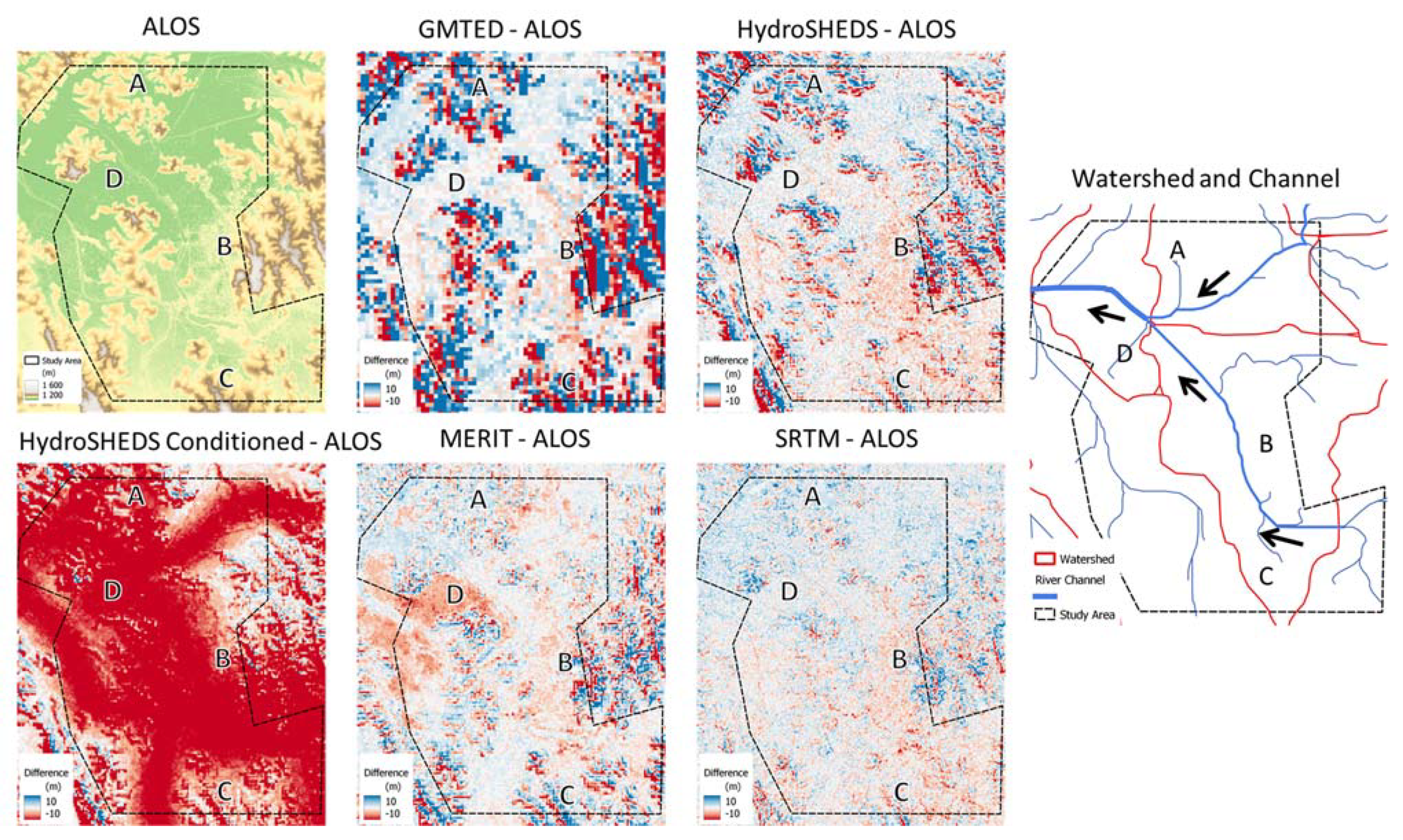
2.2.2. DEM Data
2.3. Automated Satellite-Based Surface Water Mapping
2.3.1. Image Preprocessing
2.3.2. Mapping Algorithm
- Bmax Otsu
- Edge Otsu
- Fuzzy Otsu
2.4. Automated DEM-Based Surface Water Mapping
3. Results and Discussion
3.1. Satellite-Based Surface Water Mapping Results
3.2. DEM-Based Surface Water Mapping Results
4. Discussion
5. Conclusions
Author Contributions
Funding
Data Availability Statement
Acknowledgments
Conflicts of Interest
References
- Hirabayashi, Y.; Mahendran, R.; Koirala, S.; Konoshima, L.; Yamazaki, D.; Watanabe, S.; Kim, H.; Kanae, S. Global Flood Risk under Climate Change. Nat. Clim Chang. 2013, 3, 816–821. [Google Scholar] [CrossRef]
- Sharif, H.O.; Al-Juaidi, F.H.; Al-Othman, A.; Al-Dousary, I.; Fadda, E.; Jamal-Uddeen, S.; Elhassan, A. Flood Hazards in an Urbanizing Watershed in Riyadh, Saudi Arabia. Geomat. Nat. Hazards Risk 2016, 7, 702–720. [Google Scholar] [CrossRef] [Green Version]
- Peng, B.; Huang, Q.; Vongkusolkit, J.; Gao, S.; Wright, D.B.; Fang, Z.N.; Qiang, Y. Urban Flood Mapping With Bitemporal Multispectral Imagery Via a Self-Supervised Learning Framework. IEEE J. Sel. Top. Appl. Earth Obs. Remote Sens. 2021, 14, 2001–2016. [Google Scholar] [CrossRef]
- Fang, Z.; Dolan, G.; Sebastian, A.; Bedient, P.B. Case Study of Flood Mitigation and Hazard Management at the Texas Medical Center in the Wake of Tropical Storm Allison in 2001. Nat. Hazards Rev. 2014, 15, 05014001. [Google Scholar] [CrossRef]
- Zhao, G.; Gao, H. Estimating Reservoir Evaporation Losses for the United States: Fusing Remote Sensing and Modeling Approaches. Remote Sens. Environ. 2019, 226, 109–124. [Google Scholar] [CrossRef] [Green Version]
- Nguyen, P.; Thorstensen, A.; Sorooshian, S.; Hsu, K.; AghaKouchak, A. Flood Forecasting and Inundation Mapping Using HiResFlood-UCI and Near-Real-Time Satellite Precipitation Data: The 2008 Iowa Flood. J. Hydrometeorol. 2015, 16, 1171–1183. [Google Scholar] [CrossRef]
- Munasinghe, D.; Cohen, S.; Huang, Y.-F.; Tsang, Y.-P.; Zhang, J.; Fang, Z. Intercomparison of Satellite Remote Sensing-Based Flood Inundation Mapping Techniques. J. Am. Water Resour. Assoc. 2018, 54, 834–846. [Google Scholar] [CrossRef]
- Farhadi, H.; Najafzadeh, M. Flood Risk Mapping by Remote Sensing Data and Random Forest Technique. Water 2021, 13, 3115. [Google Scholar] [CrossRef]
- Wouters, L.; Couasnon, A.; de Ruiter, M.C.; van den Homberg, M.J.; Teklesadik, A.; de Moel, H. Improving flood damage assessments in data-scarce areas by retrieval of building characteristics through UAV image segmentation and machine learning–a case study of the 2019 floods in southern Malawi. Nat. Hazards Earth Syst. Sci. 2012, 21, 3199–3218. [Google Scholar] [CrossRef]
- Schroeder, R.; McDonald, K.; Chapman, B.; Jensen, K.; Podest, E.; Tessler, Z.; Bohn, T.; Zimmermann, R. Development and Evaluation of a Multi-Year Fractional Surface Water Data Set Derived from Active/Passive Microwave Remote Sensing Data. Remote Sens. 2015, 7, 16688–16732. [Google Scholar] [CrossRef]
- Revilla-Romero, B.; Hirpa, F.; Pozo, J.; Salamon, P.; Brakenridge, R.; Pappenberger, F.; De Groeve, T. On the Use of Global Flood Forecasts and Satellite-Derived Inundation Maps for Flood Monitoring in Data-Sparse Regions. Remote Sens. 2015, 7, 15702–15728. [Google Scholar] [CrossRef] [Green Version]
- Kansara, P.; Li, W.; El-Askary, H.; Lakshmi, V.; Piechota, T.; Struppa, D.; Abdelaty Sayed, M. An Assessment of the Filling Process of the Grand Ethiopian Renaissance Dam and Its Impact on the Downstream Countries. Remote Sens. 2021, 13, 711. [Google Scholar] [CrossRef]
- Horritt, M.S. Calibration of a Two-Dimensional Finite Element Flood Flow Model Using Satellite Radar Imagery. Water Resour. Res. 2000, 36, 3279–3291. [Google Scholar] [CrossRef] [Green Version]
- Bhattacharya, B.; Mazzoleni, M.; Ugay, R. Flood Inundation Mapping of the Sparsely Gauged Large-Scale Brahmaputra Basin Using Remote Sensing Products. Remote Sens. 2019, 11, 501. [Google Scholar] [CrossRef] [Green Version]
- Massari, C.; Brocca, L.; Tarpanelli, A.; Moramarco, T. Data Assimilation of Satellite Soil Moisture into Rainfall-Runoff Modelling: A Complex Recipe? Remote Sens. 2015, 7, 11403–11433. [Google Scholar] [CrossRef] [Green Version]
- Reager, J.; Thomas, A.; Sproles, E.; Rodell, M.; Beaudoing, H.; Li, B.; Famiglietti, J. Assimilation of GRACE Terrestrial Water Storage Observations into a Land Surface Model for the Assessment of Regional Flood Potential. Remote Sens. 2015, 7, 14663–14679. [Google Scholar] [CrossRef] [Green Version]
- Fassoni-Andrade, A.C.; de Paiva, R.C.D.; Rudorff, C.d.M.; Barbosa, C.C.F.; Novo, E.M.L.d.M. High-Resolution Mapping of Floodplain Topography from Space: A Case Study in the Amazon. Remote Sens. Environ. 2020, 251, 112065. [Google Scholar] [CrossRef]
- Shastry, A.; Durand, M. Water Surface Elevation Constraints in a Data Assimilation Scheme to Infer Floodplain Topography: A Case Study in the Logone Floodplain. Geophys. Res. Lett. 2020, 47, e2020GL088759. [Google Scholar] [CrossRef]
- Feyisa, G.L.; Meilby, H.; Fensholt, R.; Proud, S.R. Automated Water Extraction Index: A New Technique for Surface Water Mapping Using Landsat Imagery. Remote Sens. Environ. 2014, 140, 23–35. [Google Scholar] [CrossRef]
- Baig, M.H.A.; Zhang, L.; Shuai, T.; Tong, Q. Derivation of a Tasselled Cap Transformation Based on Landsat 8 At-Satellite Reflectance. Remote Sens. Lett. 2014, 5, 423–431. [Google Scholar] [CrossRef]
- Lacaux, J.P.; Tourre, Y.M.; Vignolles, C.; Ndione, J.A.; Lafaye, M. Classification of Ponds from High-Spatial Resolution Remote Sensing: Application to Rift Valley Fever Epidemics in Senegal. Remote Sens. Environ. 2007, 106, 66–74. [Google Scholar] [CrossRef]
- Kaptué, A.T.; Hanan, N.P.; Prihodko, L. Characterization of the Spatial and Temporal Variability of Surface Water in the Soudan-Sahel Region of Africa: SAHEL AND SOUDANIAN SURFACE WATER BODIES. J. Geophys. Res. Biogeosci. 2013, 118, 1472–1483. [Google Scholar] [CrossRef]
- Halabisky, M.; Moskal, L.M.; Gillespie, A.; Hannam, M. Reconstructing Semi-Arid Wetland Surface Water Dynamics through Spectral Mixture Analysis of a Time Series of Landsat Satellite Images (1984–2011). Remote Sens. Environ. 2016, 177, 171–183. [Google Scholar] [CrossRef]
- Huang, C.; Chen, Y.; Zhang, S.; Li, L.; Shi, K.; Liu, R. Spatial Downscaling of Suomi NPP–VIIRS Image for Lake Mapping. Water 2017, 9, 834. [Google Scholar] [CrossRef] [Green Version]
- Isikdogan, F.; Bovik, A.C.; Passalacqua, P. Surface Water Mapping by Deep Learning. IEEE J. Sel. Top. Appl. Earth Obs. Remote Sens. 2017, 10, 4909–4918. [Google Scholar] [CrossRef]
- Acharya, T.D.; Subedi, A.; Lee, D.H. Evaluation of Machine Learning Algorithms for Surface Water Extraction in a Landsat 8 Scene of Nepal. Sensors 2019, 19, 2769. [Google Scholar] [CrossRef] [Green Version]
- DeVries, B.; Huang, C.; Lang, M.; Jones, J.; Huang, W.; Creed, I.; Carroll, M. Automated Quantification of Surface Water Inundation in Wetlands Using Optical Satellite Imagery. Remote Sens. 2017, 9, 807. [Google Scholar] [CrossRef] [Green Version]
- Huang, W.; DeVries, B.; Huang, C.; Lang, M.; Jones, J.; Creed, I.; Carroll, M. Automated Extraction of Surface Water Extent from Sentinel-1 Data. Remote Sens. 2018, 10, 797. [Google Scholar] [CrossRef] [Green Version]
- Kordelas, G.; Manakos, I.; Aragonés, D.; Díaz-Delgado, R.; Bustamante, J. Fast and Automatic Data-Driven Thresholding for Inundation Mapping with Sentinel-2 Data. Remote Sens. 2018, 10, 910. [Google Scholar] [CrossRef] [Green Version]
- Cao, H.; Zhang, H.; Wang, C.; Zhang, B. Operational Flood Detection Using Sentinel-1 SAR Data over Large Areas. Water 2019, 11, 786. [Google Scholar] [CrossRef]
- Donchyts, G.; Schellekens, J.; Winsemius, H.; Eisemann, E.; van de Giesen, N. A 30 m Resolution Surface Water Mask Including Estimation of Positional and Thematic Differences Using Landsat 8, SRTM and OpenStreetMap: A Case Study in the Murray-Darling Basin, Australia. Remote Sens. 2016, 8, 386. [Google Scholar] [CrossRef] [Green Version]
- Bazi, Y.; Melgani, F.; Bruzzone, L.; Vernazza, G. A Genetic Expectation-Maximization Method for Unsupervised Change Detection in Multitemporal SAR Imagery. Int. J. Remote Sens. 2009, 30, 6591–6610. [Google Scholar] [CrossRef]
- Dempster, A.P.; Laird, N.M.; Rubin, D.B. Maximum Likelihood from Incomplete Data Via the EM Algorithm. J. R. Stat. Soc. Ser. B Methodol. 1977, 39, 1–22. [Google Scholar] [CrossRef]
- Gstaiger, V.; Huth, J.; Gebhardt, S.; Wehrmann, T.; Kuenzer, C. Multi-Sensoral and Automated Derivation of Inundated Areas Using TerraSAR-X and ENVISAT ASAR Data. Int. J. Remote Sens. 2012, 33, 7291–7304. [Google Scholar] [CrossRef]
- Kuenzer, C.; Guo, H.; Schlegel, I.; Tuan, V.; Li, X.; Dech, S. Varying Scale and Capability of Envisat ASAR-WSM, TerraSAR-X Scansar and TerraSAR-X Stripmap Data to Assess Urban Flood Situations: A Case Study of the Mekong Delta in Can Tho Province. Remote Sens. 2013, 5, 5122–5142. [Google Scholar] [CrossRef] [Green Version]
- Bioresita, F.; Puissant, A.; Stumpf, A.; Malet, J.-P. A Method for Automatic and Rapid Mapping of Water Surfaces from Sentinel-1 Imagery. Remote Sens. 2018, 10, 217. [Google Scholar] [CrossRef] [Green Version]
- Liang, J.; Liu, D. A Local Thresholding Approach to Flood Water Delineation Using Sentinel-1 SAR Imagery. ISPRS J. Photogramm. Remote Sens. 2020, 159, 53–62. [Google Scholar] [CrossRef]
- Chen, S.; Huang, W.; Chen, Y.; Feng, M. An Adaptive Thresholding Approach toward Rapid Flood Coverage Extraction from Sentinel-1 SAR Imagery. Remote Sens. 2021, 13, 4899. [Google Scholar] [CrossRef]
- Jafarzadegan, K.; Muñoz, D.F.; Moftakhari, H.; Gutenson, J.L.; Savant, G.; Moradkhani, H. Real-Time Coastal Flood Hazard Assessment Using DEM-Based Hydrogeomorphic Classifiers. Nat. Hazards Earth Syst. Sci. 2022, 22, 1419–1435. [Google Scholar] [CrossRef]
- Cohen, S.; Brakenridge, G.R.; Kettner, A.; Bates, B.; Nelson, J.; McDonald, R.; Huang, Y.; Munasinghe, D.; Zhang, J. Estimating Floodwater Depths from Flood Inundation Maps and Topography. J. Am. Water Resour. Assoc. 2018, 54, 847–858. [Google Scholar] [CrossRef]
- Gorelick, N.; Hancher, M.; Dixon, M.; Ilyushchenko, S.; Thau, D.; Moore, R. Google Earth Engine: Planetary-Scale Geospatial Analysis for Everyone. Remote Sens. Environ. 2017, 202, 18–27. [Google Scholar] [CrossRef]
- World Bank Climate Change Knowledge Portal. Available online: https://climateknowledgeportal.worldbank.org/ (accessed on 27 July 2022).
- Randriamarolaza, L.Y.A.; Aguilar, E.; Skrynyk, O.; Vicente-Serrano, S.M.; Domínguez-Castro, F. Indices for Daily Temperature and Precipitation in Madagascar, Based on Quality-controlled and Homogenized Data, 1950–2018. Int. J. Climatol. 2022, 42, 265–288. [Google Scholar] [CrossRef]
- Madagascar: Deadly Tropical Storms Cause Flooding, Landslides. Available online: https://news.un.org/en/story/2022/01/1110532 (accessed on 22 July 2022).
- Huffman, G.J.; Stocker, E.F.; Bolvin, D.T.; Nelkin, E.J.; Tan, J. GPM IMERG Final Precipitation L3 1 month 0.1 degree x 0.1 degree V06, Greenbelt, MD, Goddard Earth Sciences Data and Information Services Center (GES DISC). 2019. Available online: https://disc.gsfc.nasa.gov/datasets/GPM_3IMERGDF_06/summary (accessed on 1 May 2022).
- Xu, H. Modification of Normalised Difference Water Index (NDWI) to Enhance Open Water Features in Remotely Sensed Imagery. Int. J. Remote Sens. 2006, 27, 3025–3033. [Google Scholar] [CrossRef]
- Twele, A.; Cao, W.; Plank, S.; Martinis, S. Sentinel-1-Based Flood Mapping: A Fully Automated Processing Chain. Int. J. Remote Sens. 2016, 37, 2990–3004. [Google Scholar] [CrossRef]
- Markert, K.N.; Markert, A.M.; Mayer, T.; Nauman, C.; Haag, A.; Poortinga, A.; Bhandari, B.; Thwal, N.S.; Kunlamai, T.; Chishtie, F.; et al. Comparing Sentinel-1 Surface Water Mapping Algorithms and Radiometric Terrain Correction Processing in Southeast Asia Utilizing Google Earth Engine. Remote Sens. 2020, 12, 2469. [Google Scholar] [CrossRef]
- Tadono, T.; Ishida, H.; Oda, F.; Naito, S.; Minakawa, K.; Iwamoto, H. Precise Global DEM Generation by ALOS PRISM. ISPRS Ann. Photogramm. Remote Sens. Spat. Inf. Sci. 2014, 2, 71. [Google Scholar] [CrossRef] [Green Version]
- Lehner, B.; Verdin, K.; Jarvis, A. New Global Hydrography Derived From Spaceborne Elevation Data. Eos Trans. AGU 2008, 89, 93. [Google Scholar] [CrossRef]
- Yamazaki, D.; Ikeshima, D.; Tawatari, R.; Yamaguchi, T.; O’Loughlin, F.; Neal, J.C.; Sampson, C.C.; Kanae, S.; Bates, P.D. A High-Accuracy Map of Global Terrain Elevations: Accurate Global Terrain Elevation Map. Geophys. Res. Lett. 2017, 44, 5844–5853. [Google Scholar] [CrossRef] [Green Version]
- Danielson, J.J.; Gesch, D.B. Global Multi-Resolution Terrain Elevation Data 2010 (GMTED2010); US Department of the Interior, US Geological Survey: Washington, DC, USA, 2011. [Google Scholar]
- Farr, T.G.; Rosen, P.A.; Caro, E.; Crippen, R.; Duren, R.; Hensley, S.; Kobrick, M.; Paller, M.; Rodriguez, E.; Roth, L.; et al. The Shuttle Radar Topography Mission. Rev. Geophys. 2007, 45, RG2004. [Google Scholar] [CrossRef] [Green Version]
- Foga, S.; Scaramuzza, P.L.; Guo, S.; Zhu, Z.; Dilley, R.D.; Beckmann, T.; Schmidt, G.L.; Dwyer, J.L.; Joseph Hughes, M.; Laue, B. Cloud Detection Algorithm Comparison and Validation for Operational Landsat Data Products. Remote Sens. Environ. 2017, 194, 379–390. [Google Scholar] [CrossRef]
- Jong-Sen, L.; Jen-Hung, W.; Ainsworth, T.L.; Kun-Shan, C.; Chen, A.J. Improved Sigma Filter for Speckle Filtering of SAR Imagery. IEEE Trans. Geosci. Remote Sens. 2009, 47, 202–213. [Google Scholar] [CrossRef]
- Beauchemin, M.; Thomson, K.P.B.; Edwards, G. Optimization of the Gamma-Gamma MAP Filter for SAR Image Clutters. Int. J. Remote Sens. 1996, 17, 1063–1067. [Google Scholar] [CrossRef]
- Lee, J.-S. Refined Filtering of Image Noise Using Local Statistics. Comput. Graph. Image Process. 1981, 15, 380–389. [Google Scholar] [CrossRef]
- Vollrath, A.; Mullissa, A.; Reiche, J. Angular-Based Radiometric Slope Correction for Sentinel-1 on Google Earth Engine. Remote Sens. 2020, 12, 1867. [Google Scholar] [CrossRef]
- Otsu, N. A Threshold Selection Method from Gray-Level Histograms. IEEE Trans. Syst. Man Cybern. 1979, 9, 62–66. [Google Scholar] [CrossRef] [Green Version]
- Rambabu, P.; Raju, C.N. The Optimal Thresholding Technique for Image Segmentaion Using Fuzzy Otsu Method. IJ-AI 2015, 4, 81. [Google Scholar] [CrossRef]
- Canny, J. A Computational Approach to Edge Detection. IEEE Trans. Pattern Anal. Mach. Intell. 1986, PAMI-8, 679–698. [Google Scholar] [CrossRef]
- Fuzzy Membership (Spatial Analyst)—ArcGIS Pro|Documentation. Available online: https://pro.arcgis.com/en/pro-app/2.8/tool-reference/spatial-analyst/fuzzy-membership.htm (accessed on 22 July 2022).
- Cohen, S.; Raney, A.; Munasinghe, D.; Loftis, J.D.; Molthan, A.; Bell, J.; Rogers, L.; Galantowicz, J.; Brakenridge, G.R.; Kettner, A.J.; et al. The Floodwater Depth Estimation Tool (FwDET v2.0) for Improved Remote Sensing Analysis of Coastal Flooding. Nat. Hazards Earth Syst. Sci. 2019, 19, 2053–2065. [Google Scholar] [CrossRef] [Green Version]
- Peter, B.G.; Cohen, S.; Lucey, R.; Munasinghe, D.; Raney, A.; Brakenridge, G.R. Google Earth Engine Implementation of the Floodwater Depth Estimation Tool (FwDET-GEE) for Rapid and Large Scale Flood Analysis. IEEE Geosci. Remote Sens. Lett. 2022, 19, 1–5. [Google Scholar] [CrossRef]
- Li, W.; El-Askary, H.; Lakshmi, V.; Piechota, T.; Struppa, D. Earth Observation and Cloud Computing in Support of Two Sustainable Development Goals for the River Nile Watershed Countries. Remote Sens. 2020, 12, 1391. [Google Scholar] [CrossRef]
- Brown, C.F.; Brumby, S.P.; Guzder-Williams, B.; Birch, T.; Hyde, S.B.; Mazzariello, J.; Czerwinski, W.; Pasquarella, V.J.; Haertel, R.; Ilyushchenko, S.; et al. Dynamic World, Near Real-Time Global 10 m Land Use Land Cover Mapping. Sci. Data 2022, 9, 251. [Google Scholar] [CrossRef]
- El-Askary, H.; Fawzy, A.; Thomas, R.; Li, W.; LaHaye, N.; Linstead, E.; Piechota, T.; Struppa, D.; Sayed, M.A. Assessing the Vertical Displacement of the Grand Ethiopian Renaissance Dam during Its Filling Using DInSAR Technology and Its Potential Acute Consequences on the Downstream Countries. Remote Sens. 2021, 13, 4287. [Google Scholar] [CrossRef]
- Braun, A. Retrieval of Digital Elevation Models from Sentinel-1 Radar Data—Open Applications, Techniques, and Limitations. Open Geosci. 2021, 13, 532–569. [Google Scholar] [CrossRef]
- Li, D.; Fang, Z.N.; Bedient, P.B. Flood Early Warning Systems under Changing Climate and Extreme Events. In Climate Change and Extreme Events; Elsevier: Amsterdam, The Netherlands, 2021; pp. 83–103. ISBN 978-0-12-822700-8. [Google Scholar]
- Sanders, W.; Li, D.; Li, W.; Fang, Z.N. Data-Driven Flood Alert System (FAS) Using Extreme Gradient Boosting (XGBoost) to Forecast Flood Stages. Water 2022, 14, 747. [Google Scholar] [CrossRef]
- Fang, Z.; Bedient, P.B.; Benavides, J.; Zimmer, A.L. Enhanced Radar-Based Flood Alert System and Floodplain Map Library. J. Hydrol. Eng. 2008, 13, 926–938. [Google Scholar] [CrossRef]


| Satellite | Provider | Sensor | Polarization/Band | Resolution | Wavelength |
|---|---|---|---|---|---|
| Sentinel-1 | ESA | C-band SAR | VV | 10 m | ~5.55 cm |
| Sentinel-2 | ESA | Multispectral Instrument (MSI) | Green | 10 m | ~0.56 μm |
| SWIR | 20 m | ~1.61 μm | |||
| Landsat-7 | NASA | Enhanced Thematic Mapper Plus (ETM+) | Green | 30 m | 0.52–0.60 μm |
| SWIR | 30 m | 1.55–1.75 μm | |||
| Landsat-8 | NASA | Operational Land Imager (OLI) | Green | 30 m | 0.53–0.59 μm |
| SWIR | 30 m | 1.57–1.65 μm | |||
| Landsat-9 | NASA | Operational Land Imager 2 (OLI 2) | Green | 30 m | 0.53–0.59 μm |
| SWIR | 30 m | 1.57–1.65 μm |
| Satellite | Provider | Resolution | Reference |
|---|---|---|---|
| ALOS | JAXA | 30 m | [49] |
| HydroSHEDS | WWF | 93 m | [50] |
| HydroSHEDS Hydrologically Conditioned | WWF | 93 m | [50] |
| MERIT | Dai Yamazaki | 93 m | [51] |
| GMTED 2010 | USGS | 232 m | [52] |
| SRTM | NASA/USGS | 30 m | [53] |
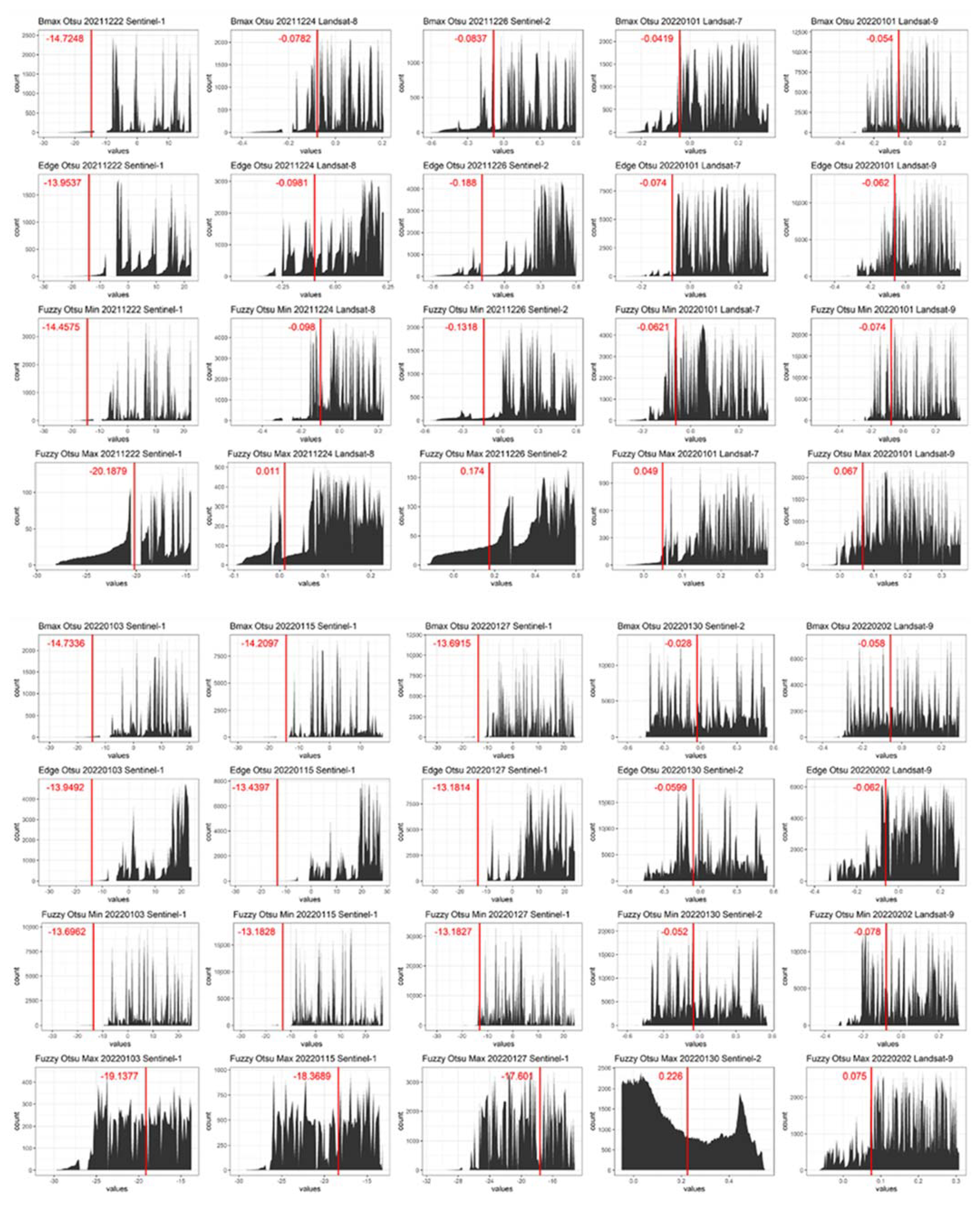
| Date | Satellite | Bmax Otsu | Edge Otsu | Fuzzy Otsu | |||
|---|---|---|---|---|---|---|---|
| Threshold | Area (km2) | Threshold | Area (km2) | Threshold | Area (km2) | ||
| 22 December 2021 | Sentinel-1 | −14.7248 | 4.03 | −13.9537 | 4.69 | −17.3227 | 2.74 |
| 24 December 2021 | Landsat-8 | −0.0782 | 22.1 | −0.0981 | 31.71 | −0.0435 | 40.92 |
| 26 December 2021 | Sentinel-2 * | −0.0837 | 6.53 | −0.188 | 13.65 | 0.0211 | 5.26 |
| 1 January 2022 | Landsat-9 | −0.054 | 40.76 | −0.062 | 46.47 | −0.0035 | 55.23 |
| 1 January 2022 | Landsat-7 * | −0.0419 | 5.26 | −0.074 | 6.72 | −0.00655 | 6.85 |
| 3 January 2022 | Sentinel-1 | −14.7336 | 6.26 | −13.9492 | 7.51 | −16.41695 | 4.56 |
| 15 January 2022 | Sentinel-1 | −14.2097 | 11.05 | −13.4397 | 13.27 | −15.77585 | 7.85 |
| 27 January 2022 | Sentinel-1 | −13.6915 | 40.07 | −13.1814 | 42.69 | −15.39185 | 32.54 |
| 30 January 2022 | Sentinel-2 * | −0.028 | 63.08 | −0.0599 | 69.88 | 0.087 | 52.79 |
| 2 February 2022 | Landsat-9 | −0.058 | 73.41 | −0.062 | 75.3 | −0.0015 | 80.21 |
Disclaimer/Publisher’s Note: The statements, opinions and data contained in all publications are solely those of the individual author(s) and contributor(s) and not of MDPI and/or the editor(s). MDPI and/or the editor(s) disclaim responsibility for any injury to people or property resulting from any ideas, methods, instructions or products referred to in the content. |
© 2023 by the authors. Licensee MDPI, Basel, Switzerland. This article is an open access article distributed under the terms and conditions of the Creative Commons Attribution (CC BY) license (https://creativecommons.org/licenses/by/4.0/).
Share and Cite
Li, W.; Li, D.; Fang, Z.N. Intercomparison of Automated Near-Real-Time Flood Mapping Algorithms Using Satellite Data and DEM-Based Methods: A Case Study of 2022 Madagascar Flood. Hydrology 2023, 10, 17. https://doi.org/10.3390/hydrology10010017
Li W, Li D, Fang ZN. Intercomparison of Automated Near-Real-Time Flood Mapping Algorithms Using Satellite Data and DEM-Based Methods: A Case Study of 2022 Madagascar Flood. Hydrology. 2023; 10(1):17. https://doi.org/10.3390/hydrology10010017
Chicago/Turabian StyleLi, Wenzhao, Dongfeng Li, and Zheng N. Fang. 2023. "Intercomparison of Automated Near-Real-Time Flood Mapping Algorithms Using Satellite Data and DEM-Based Methods: A Case Study of 2022 Madagascar Flood" Hydrology 10, no. 1: 17. https://doi.org/10.3390/hydrology10010017