1. Introduction
Methods to predict phase equilibria are crucial for the design of industrial separation processes, which typically constitute 40–70% of both the capital and operating cost of a chemical plant. Separation processes are non-spontaneous processes requiring an external “separating agent”, typically either energy or a solvent, which make them expensive [
1]. Here, we considered vapor–liquid separation processes, which include distillation, absorption, and stripping. Distillation alone constitutes approximately 90–95% of the separation processes used in practice and, in the United States, accounts for approximately 11% of all in-plant energy consumed [
2,
3].
Solubility-parameter-based methods have long been utilized for early-stage process conceptualization and design applications as a result of their ability to both predict the phase equilibrium and shed light on the underlying intermolecular interactions [
4,
5,
6,
7,
8,
9,
10,
11,
12]. When using these methods to compute limiting activity coefficients, we decompose the log limiting activity coefficient into the sum of a combinatorial (COMB) and residual (RES) contribution, where the COMB contribution results from size and shape dissimilarities between the components in the system and the RES contribution results from intermolecular interactions. The COMB contribution may be computed using available athermal solution theories, such as the Flory–Huggins or Flory–Huggins–Staverman–Guggenheim equations [
4,
13,
14].
The earliest solubility parameter method to predict the RES contribution was Hildebrand and Scatchard’s “Regular Solution Theory” (RST). However, RST is limited in that it can only predict positive contributions, as well as being limited to modeling dispersion interactions [
4,
5]. Solubility parameter methods have been greatly improved by splitting the solubility parameter into a sum of contributions [
5,
11]. Perhaps the most-well-known of these methods is the Hansen solubility parameter (HSP), which accounts for dispersion, polar, and hydrogen bonding interactions [
6]. This results in an expression of the RES contribution of the limiting activity coefficient of the form:
where
is the RES contribution of the limiting activity coefficient of Component 2,
R is the molar gas constant,
T is the absolute temperature,
is the pure component molar volume of Component 2,
is the pure component solubility parameter of component
i, which accounts for the dispersion interactions,
is the pure component solubility parameter of component
i, which accounts for the polar interactions, and
is the pure component solubility parameter of component
i, which accounts for hydrogen bonding (or association), where
. Within the hydrogen bonding term,
corresponds to self-association, where
accounts for the hydrogen bond donating ability and
accounts for the hydrogen bond accepting ability of component
i. However, HSP is still limited in that it can only predict positive RES contributions. Tijssen et al. [
12] overcame this limitation by splitting the hydrogen bonding term, resulting in [
12].
This expression forms the basis of modified separation of cohesive energy density (MOSCED), which we utilized here [
15,
16,
17,
18,
19,
20,
21,
22,
23,
24]. It should be noted that this splitting has recently been suggested to improve the accuracy of the HSP [
10].
The limiting activity coefficient accounts for solute–solvent and solvent–solvent interactions and corresponds to the maximum deviation from the ideal solution behavior. Moreover, the limiting activity can be used to predict a wide range of phase equilibria for early-stage design applications [
25]. For example, Henry’s constant for Component 2 in 1 (
) may be computed as [
24]
and the fundamental solvation free energy of Component 2 in 1 (
) [
24]:
where
T and
P are the temperature and pressure, respectively,
is the vapor pressure of pure Component 2,
R is the molar gas constant, and
is the molar volume of Component 1, where we made the standard assumptions that the vapor phase is an ideal gas and the Poynting correction is negligible such that the pure component fugacity is equal to the pure component vapor pressure. Likewise, for the case of isothermal vapor–liquid equilibrium, it can be shown that, for a mono-azeotropic system, for a system to exhibit a minimum boiling azeotrope [
26,
27]:
and for a system to exhibit a maximum boiling azeotrope [
26,
27]:
where
is the vapor pressure of pure Component 1 and Component 1 corresponds to the most-volatile component (
). It is additionally possible to use limiting activity coefficients to parameterize a binary interaction excess Gibbs free energy model, which may then be used to extrapolate to finite concentrations. For the case of Wilson’s equation, we have [
4,
24,
28]
where
and
are adjustable parameters, which may be related to the binary (intermolecular) interaction parameters (BIPs) of the system (
and
):
At infinite dilution, Equation (
7) reduces to
which can be used to solve for parameters
and
. This may, in turn, be used to model vapor–liquid equilibrium, where
where
and
are the vapor phase mole fraction of Components 1 and 2, respectively, and recall
and
.
Be that as it may, Equations (
3)–(
6) and (
10) all require knowledge of the pure component vapor pressure. While the vapor pressure is available for a wide range of fluids, the ability to predict vapor pressure using MOSCED parameters would be of great value for early-stage process conceptualization and design applications. It has previously been shown that MOSCED parameters may be used to correlate the enthalpy of vaporization [
29,
30]. Given the relationship between the enthalpy of vaporization and log vapor pressure via the Clapeyron equation, we hypothesized that the correlation of the vapor pressure should also be possible. Likewise, Abraham solute descriptors have been used to correlate a wide range of thermophysical properties, including the enthalpy of vaporization and vapor pressure [
31,
32,
33]. Since MOSCED parameters correspond to physical interactions, we expected that it should likewise be possible to use them as descriptors to correlate and predict vapor pressure.
Recently in 2005, MOSCED was subject to a “revision”, wherein the literature was surveyed and the parameters were regressed for 130 organic solvents, water, 2-room-temperature ionic liquids (ILs), and 5 non-condensable gases using experimental limiting activity coefficients [
20]; this was recently expanded to an additional 33 1-
n-alkyl-3-methylimidazolium-based ILs [
34,
35]. The further expansion of MOSCED is limited by the availability of experimental limiting activity coefficients. The ability to use MOSCED to correlate pure component properties could be of additional value in that it would allow one to incorporate additional data into the regression of new parameters. This has been demonstrated previously for MOSCED with the use of the enthalpy of vaporization [
36]. Additionally, recent efforts have been made to predict MOSCED parameters devoid of experimental data. This includes the use of molecular simulation and electronic structure calculation to generate reference data [
30,
36,
37,
38,
39] and traditional group contribution methods [
29,
36]. The present study is complementary to this work, wherein it presents the opportunity to predict phase equilibrium for early stage process conceptualization and design applications.
Know that many excellent methods exist to predict pure component properties from molecular structures. For example, the group contribution method of Gani and co-workers can be used to predict a wide range of pure component properties [
40,
41]. This includes the critical temperature, pressure, and acentric factor, which, in turn, could be used to predict vapor pressure using a cubic equation of state. Likewise, Gharagheizi et al. [
42] recently developed a group contribution/machine learning method to predict vapor pressure directly. As mentioned earlier, Abraham solute descriptors have been used to correlate a wide range of thermophysical properties including vapor pressure [
32]. The goal of the present study was to assess the ability to use MOSCED parameters to correlate and predict pure component properties, specifically the enthalpy of vaporization and vapor pressure. This would allow for the prediction of phase equilibrium using only MOSCED parameters for early-stage process conceptualization and design applications and, additionally, provides the opportunity to incorporate additional data into the parameterization of MOSCED. Moreover, in general, the ability to predict pure component properties and to provide molecular-level insight via the solubility parameter would be of great utility.
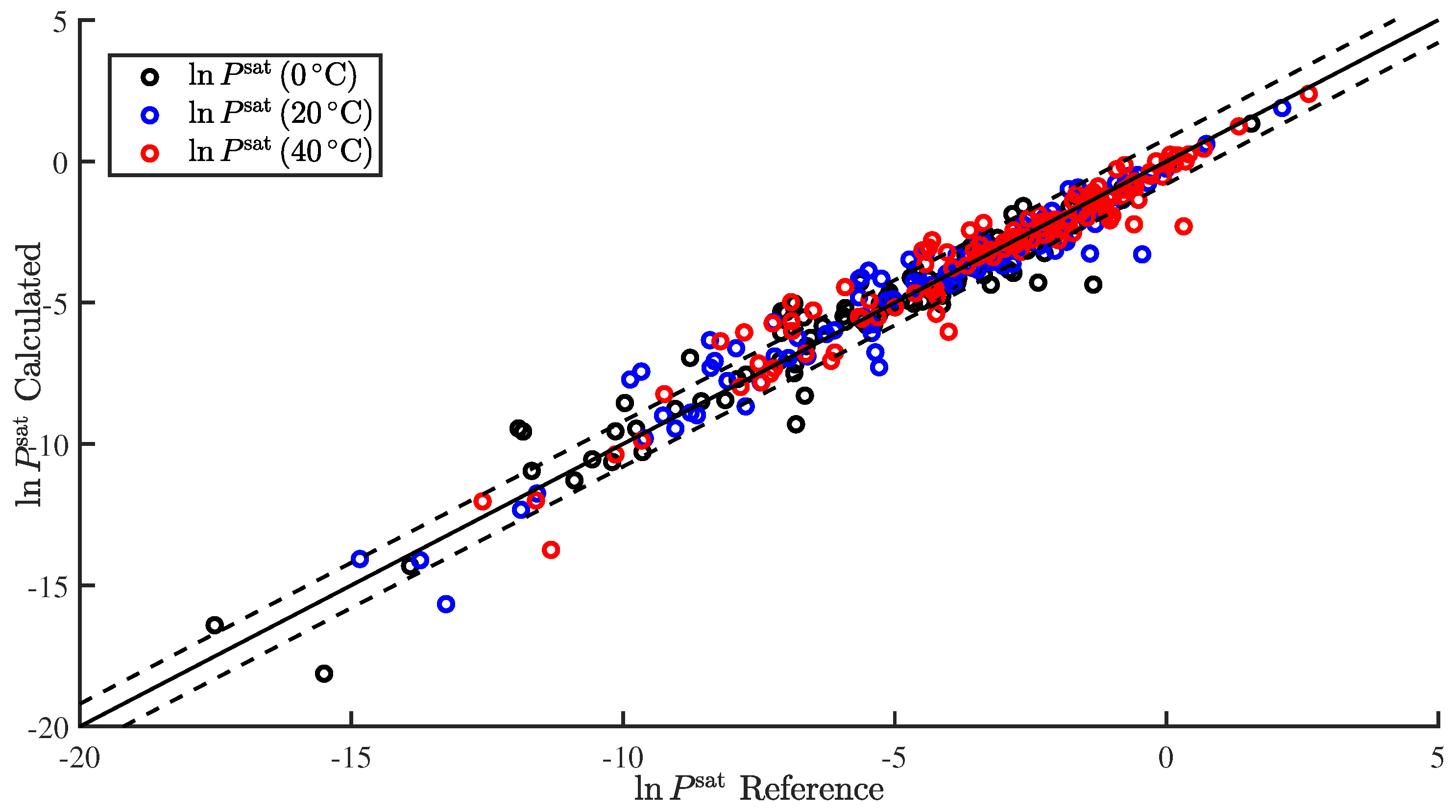
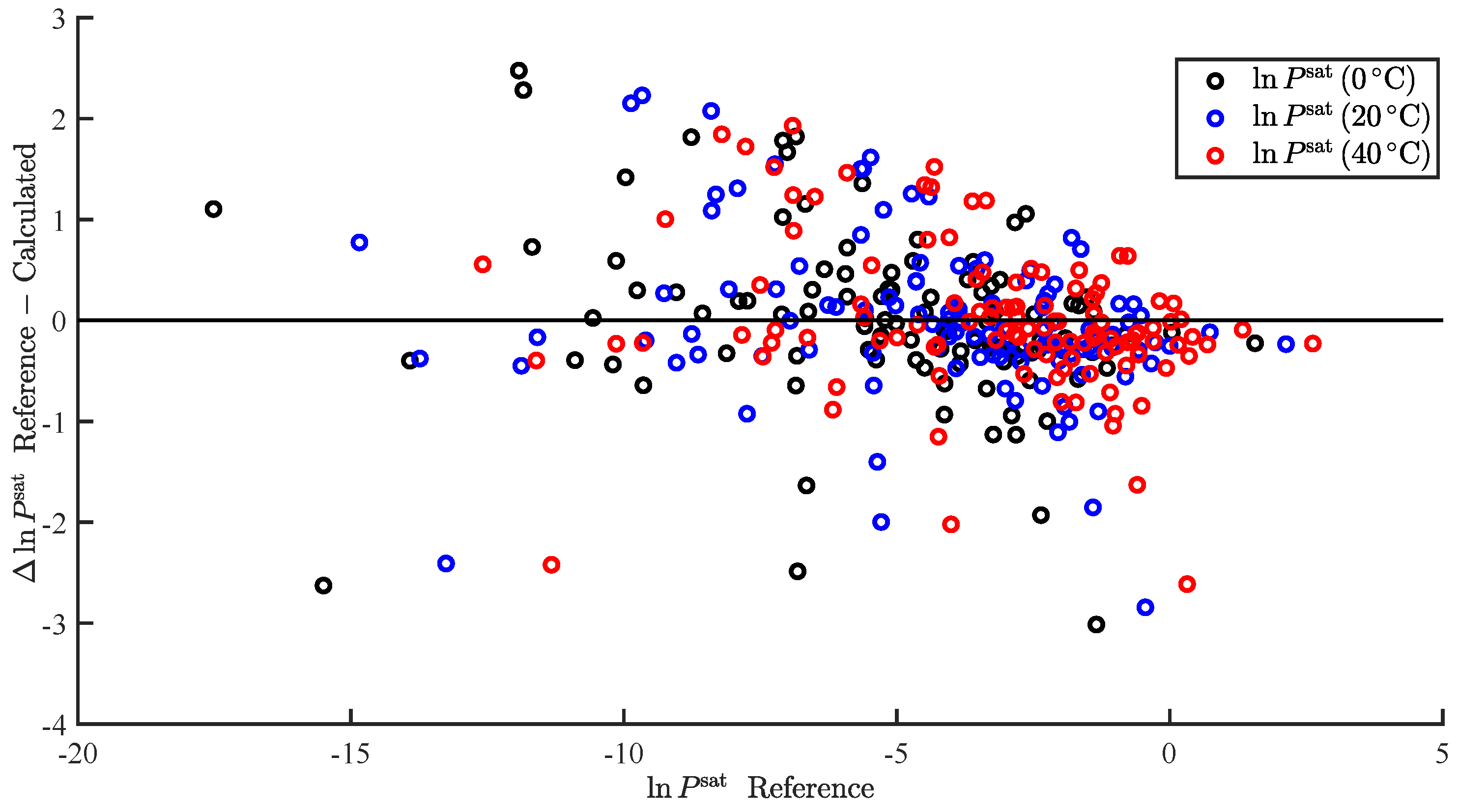
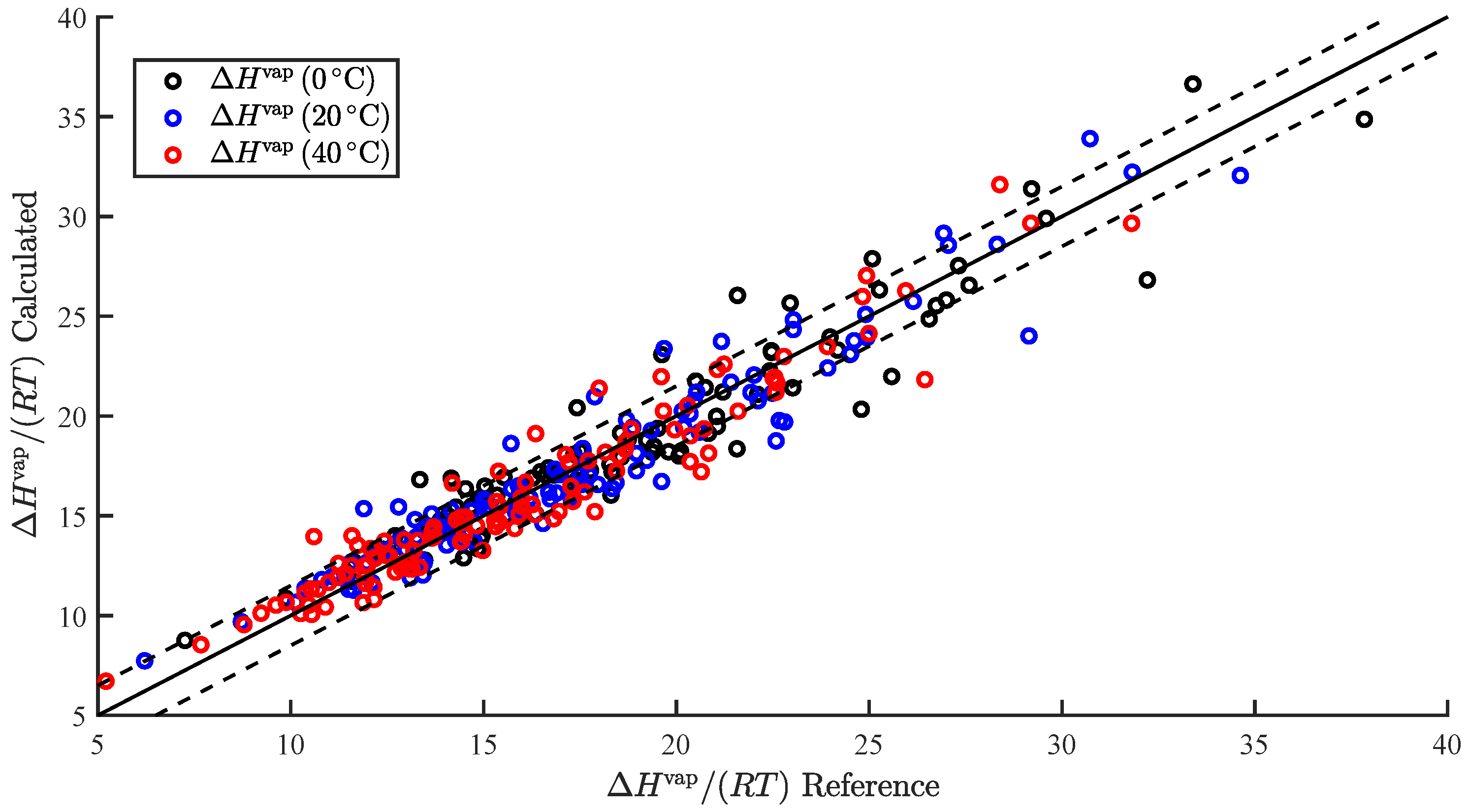
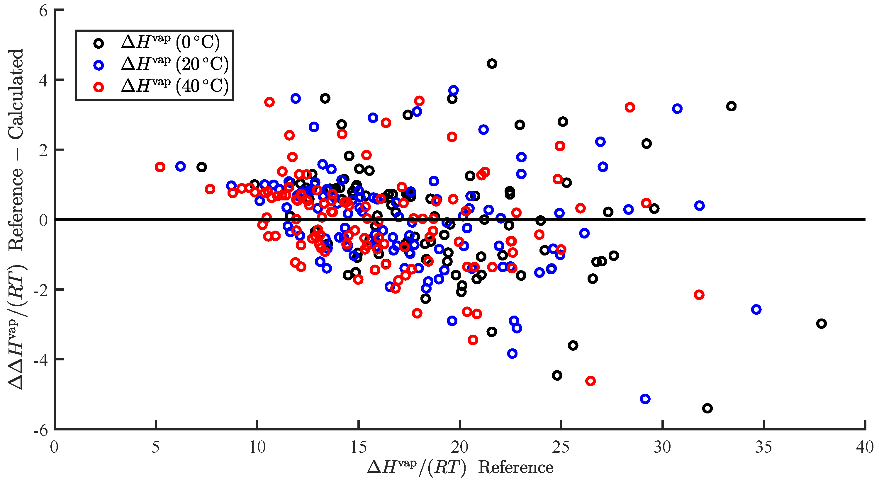
In the present study, we demonstrated the ability to successfully correlate the enthalpy of vaporization and vapor pressure at a specific temperature. Furthermore, we demonstrated the ability to use the predicted enthalpy of vaporization to extrapolate the predicted vapor pressure to additional temperatures. This was applied to predict and . We also summarize our results, wherein we attempted to correlate additional pure component properties, but with limited success.
4. Summary and Conclusions
In the present study, we demonstrated and assessed the ability of MOSCED to correlate the enthalpy of vaporization and vapor pressure at a specific temperature using multiple linear regression. MOSCED is a solubility-parameter-based method, wherein the parameters correspond to specific, physical intermolecular interactions. In this way, MOSCED can be used to both predict phase equilibria and shed light on the underlying intermolecular interactions, which is advantageous for early-stage process development and design.
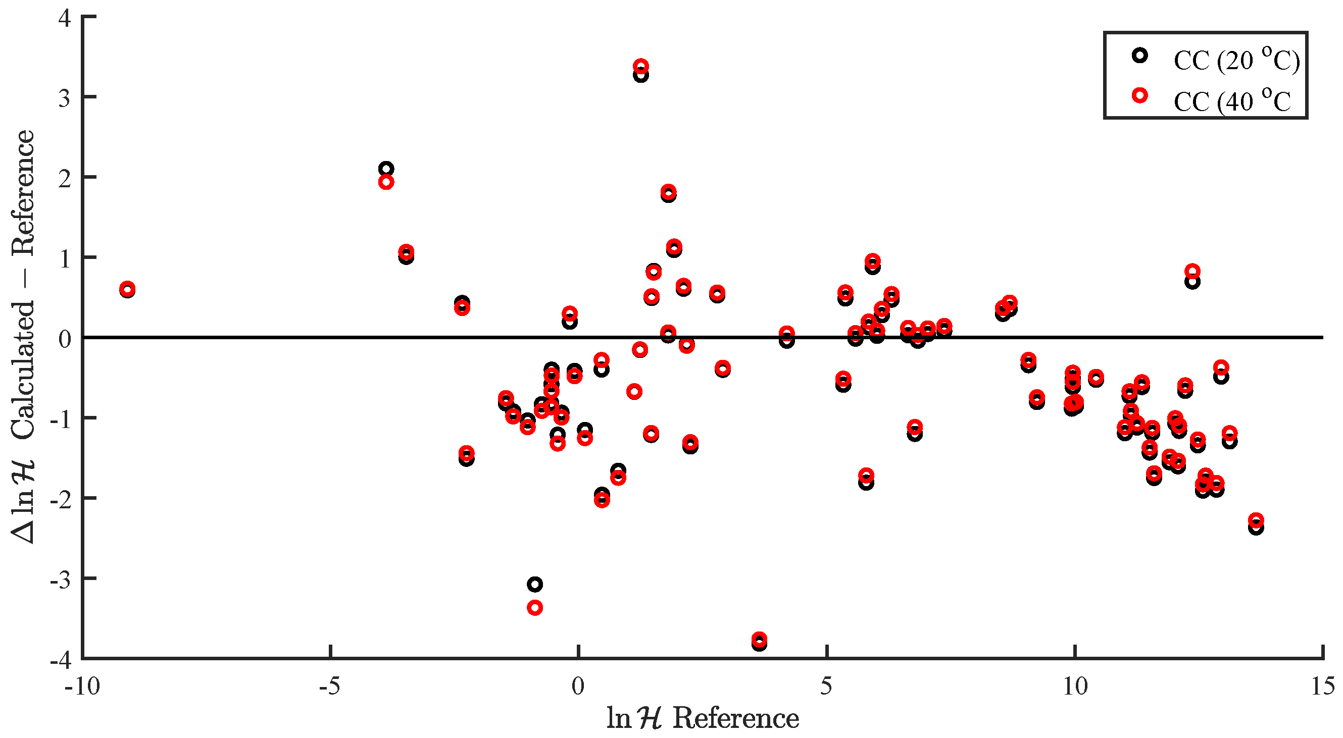
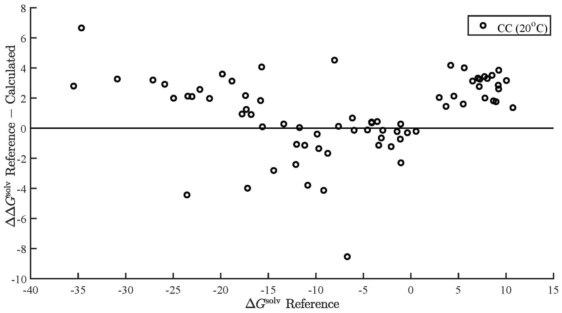
MOSCED is based on the theory that the cohesive energy may be separated into individual contributions (due to specific intermolecular interactions), which are additive. The cohesive energy is directly related to the enthalpy of vaporization, and MOSCED has, in turn, been shown previously to well correlate the enthalpy of vaporization. Here, we showed that MOSCED is additionally able to correlate the log vapor pressure. While MOSCED can be used to predict limiting activity coefficients, the additional ability to predict vapor pressure extends MOSCED to be able to predict vapor–liquid phase equilibrium devoid of reference data. Here, this was demonstrated by using MOSCED to predict the Henry’s constant and solvation free energy of organic solutes in water. While the errors in the predicted Henry’s constant were slightly larger when MOSCED was used to additionally predict the vapor pressure, the difference was small and still superior to the use of mod-UNIFAC. The same was true with the solvation free energy; only the difference between the use of reference and MOSCED predicted vapor pressures was insignificant. In the most-recent MOSCED revision, parameters were regressed for 130 organic compounds. This was limited due to the availability of reference limiting activity coefficients. In addition to being able to make phase equilibrium predictions, the ability to correlate the enthalpy of vaporization and vapor pressure offers the opportunity to include additional properties in the regression of MOSCED parameters.
Given the success in correlating the enthalpy of vaporization and vapor pressure, we attempted to correlate a wide range of physical properties using similar expressions. While, in some cases, the results were reasonable, they were inferior to the correlations of the enthalpy of vaporization and vapor pressure. Future efforts will be needed to improve the correlations.


