

Prediction of Particle Size Distribution of Mill Products Using Artificial Neural Networks

Abstract
:1. Introduction
2. Materials and Methods
2.1. Materials
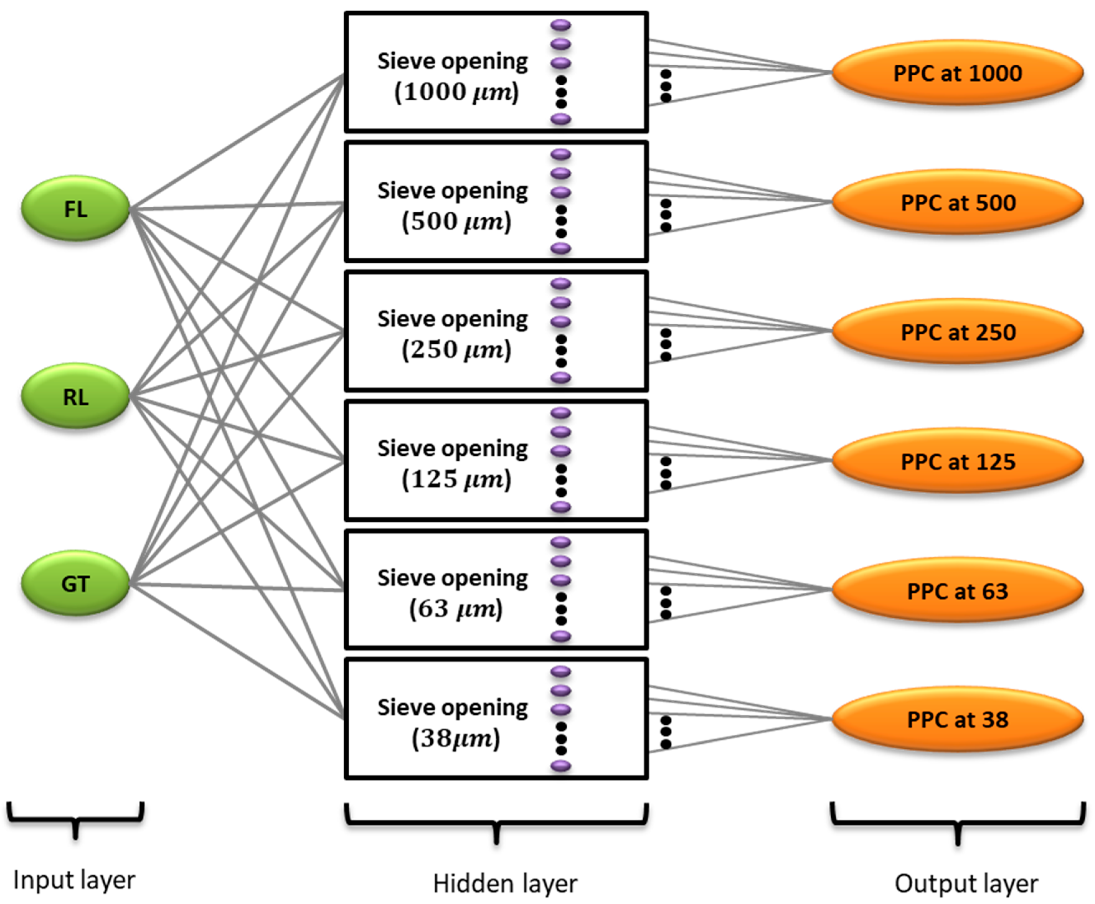
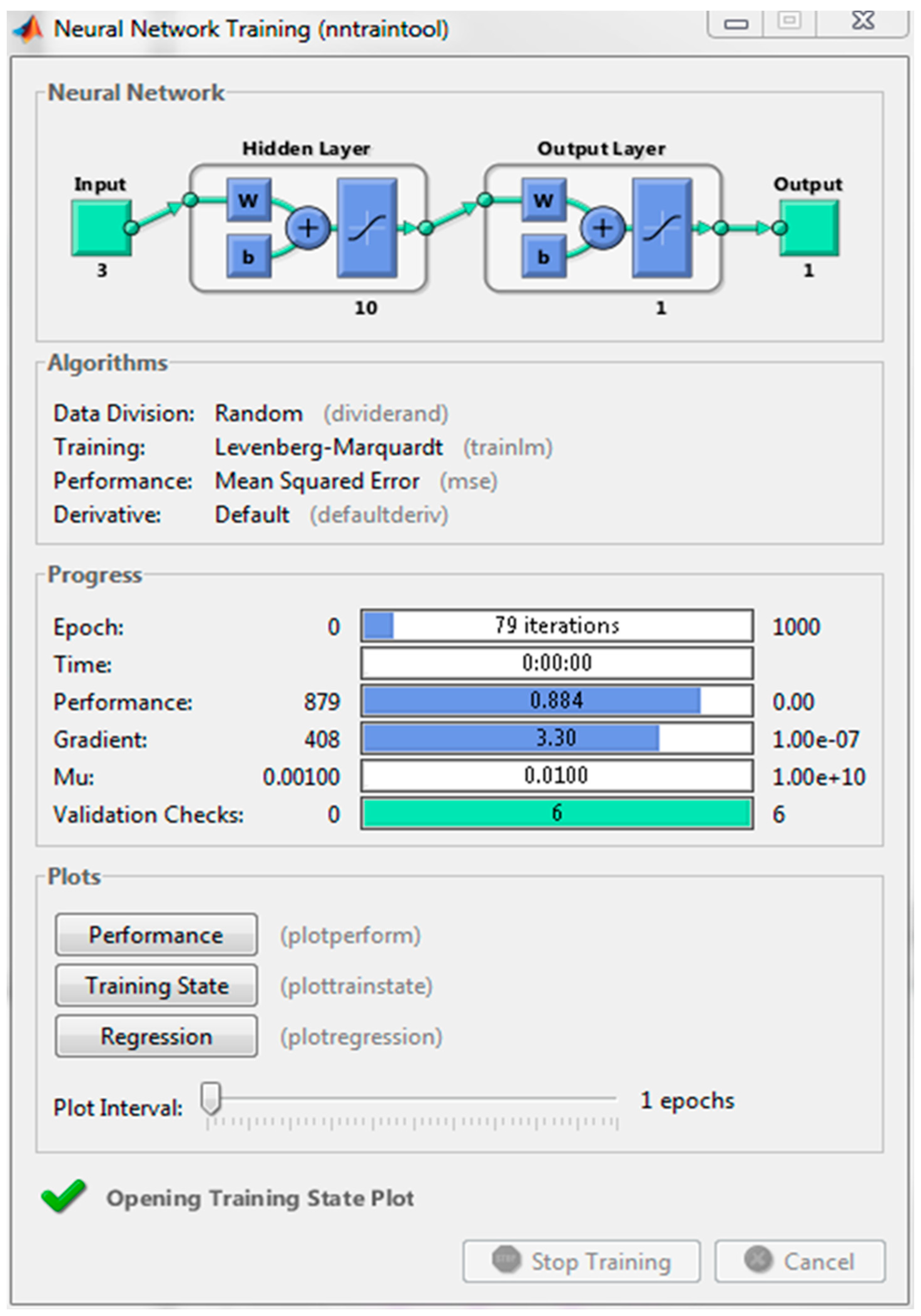
2.2. Methods-ANN Model Predicting Percentage Passing Cumulative
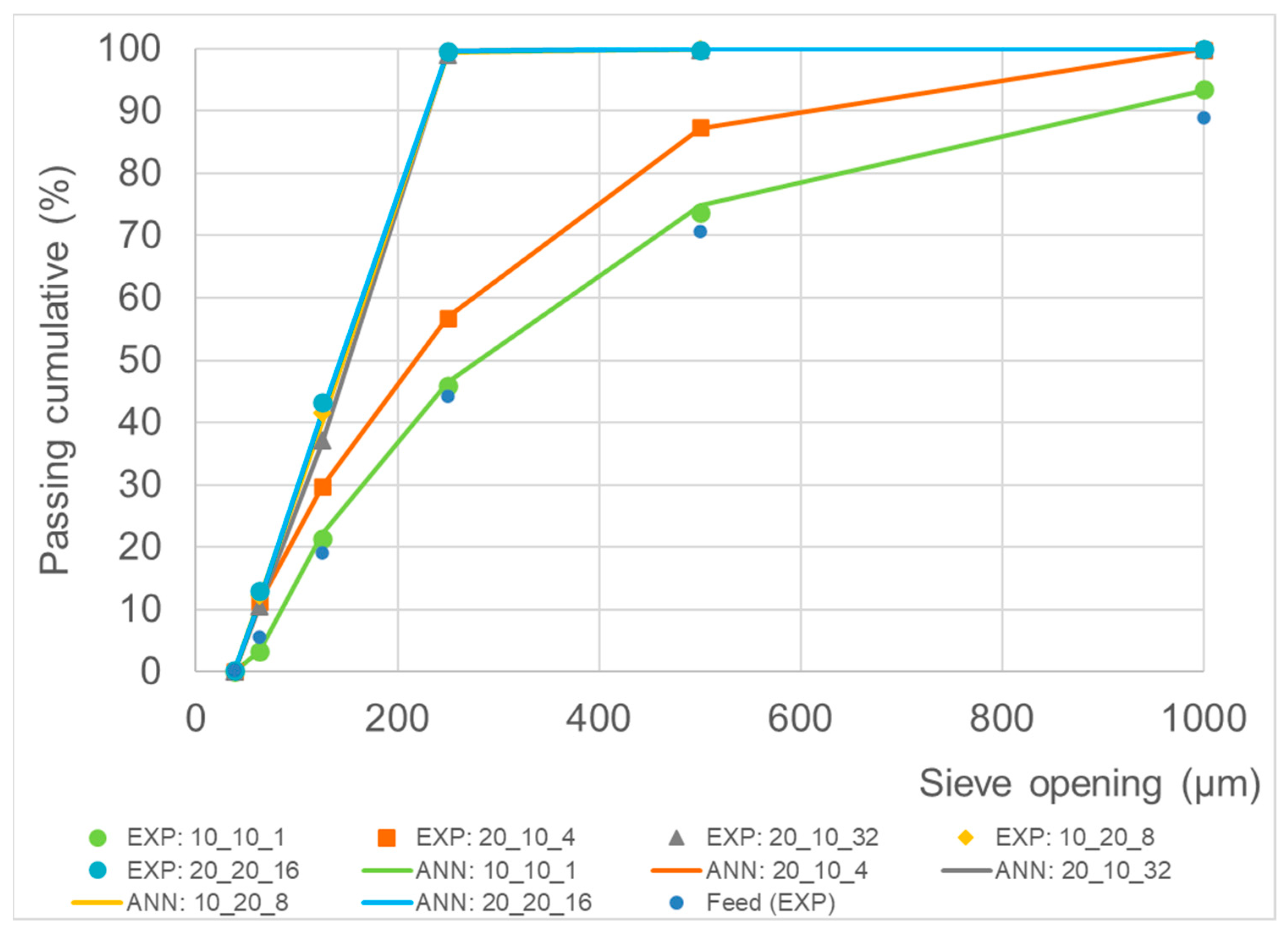
3. Results and Discussion
4. Conclusions
Author Contributions
Funding
Institutional Review Board Statement
Informed Consent Statement
Data Availability Statement
Conflicts of Interest
References
- Government of Canada. Tackling Comminution, the Largest Energy Consumer. Available online: https://www.nrcan.gc.ca/our-natural-resources/minerals-mining/mining-resources/tackling-comminution-largest-energy-consumer/18296 (accessed on 10 October 2022).
- Towell, G.G.; Shavlik, J.W. Knowledge-based artificial neural networks. Artif. Intell. 1994, 70, 119–165. [Google Scholar] [CrossRef]
- World Coal Association. Coal Statistics. 2012. Available online: http://www.worldcoal.org/resources/coal-statistics/ (accessed on 4 April 2013).
- Otsuki, A.; Miller, T. Experimental Investigation on Safer Frother Option for Coal Flotation. Curr. Work. Miner. Process. 2019, 1, 1–12. [Google Scholar] [CrossRef]
- Otsuki, A.; Miller, T. Safer Frother Option for Coal Flotation—A Review. Curr. Work. Miner. Process. 2019, 1, 21–29. [Google Scholar] [CrossRef]
- Aaron, N.; Luttrell, G.H. A review of state-of-the-art processing operations in coal preparation. Int. J. Min. Sci. Technol. 2015, 25, 511–521. [Google Scholar]
- Vadood, M.; Haji, A. Application of ANN Weighted by Optimization Algorithms to Predict the Color Coordinates of Cellulosic Fabric in Dyeing with Binary Mix of Natural Dyes. Coatings 2022, 12, 1519. [Google Scholar] [CrossRef]
- Soomro, A.A.; Mokhtar, A.A.; Salilew, W.M.; Abdul Karim, Z.A.; Abbasi, A.; Lashari, N.; Jameel, S.M. Machine Learning Approach to Predict the Performance of a Stratified Thermal Energy Storage Tank at a District Cooling Plant Using Sensor Data. Sensors 2022, 22, 7687. [Google Scholar] [CrossRef]
- Irandegani, M.A.; Zhang, D.; Shadabfar, M. Probabilistic assessment of axial load-carrying capacity of FRCM-strengthened concrete columns using artificial neural network and Monte Carlo simulation. Case Stud. Constr. Mater. 2022, 17, e01248. [Google Scholar] [CrossRef]
- Sarir, P.; Armaghani, D.J.; Jiang, H.; Sabri, M.M.S.; He, B.; Ulrikh, D.V. Prediction of Bearing Capacity of the Square Concrete-Filled Steel Tube Columns: An Application of Metaheuristic-Based Neural Network Models. Materials 2022, 15, 3309. [Google Scholar] [CrossRef]
- Jang, H.; Topal, E. A review of soft computing technology applications in several mining problems. Appl. Soft Comput. 2014, 22, 638–651. [Google Scholar] [CrossRef]
- Alam, M.A.; Ya, H.H.; Azeem, M.; Yusuf, M.; Soomro, I.A.; Masood, F.; Shozib, I.A.; Sapuan, S.M.; Akhter, J. Artificial Neural Network Modeling to Predict the Effect of Milling Time and TiC Content on the Crystallite Size and Lattice Strain of Al7075-TiC Composites Fabricated by Powder Metallurgy. Crystals 2022, 12, 372. [Google Scholar] [CrossRef]
- Shi, X.; Huang, D.; Zhou, J.; Zhang, S. Combined ANN Prediction Model for Rock Fragmentation Distribution due to Blasting. J. Inf. Comput. Sci. 2013, 10, 3511–3518. [Google Scholar] [CrossRef]
- Yu, H.; Fu, J.; Dang, L.; Cheong, Y.; Tan, H.; Wei, H. Prediction of the particle size distribution parameters in a high shear granulation process using a key parameter definition combined artificial neural network model. Ind. Eng. Chem. Res. 2015, 54, 10825–10834. [Google Scholar] [CrossRef]
- Weerasekara, N.S.; Liu, L.X.; Powell, M.S. Estimating energy in grinding using DEM modelling. Miner. Eng. 2016, 85, 23–33. [Google Scholar] [CrossRef] [Green Version]
- Esnault, V.P.B.; Zhou, H.; Heitzmann, D. New population balance model for predicting particle size evolution in compression grinding. Miner. Eng. 2015, 73, 7–15. [Google Scholar] [CrossRef]
- Kor, M.; Abkhoshk, E.; Tao, D.; Chen, G.L.; Modarres, H. Modeling and optimization of high chromium alloy wear in phosphate laboratory grinding mill with fuzzy logic and particle swarm optimization technique. Miner. Eng. 2010, 23, 713–719. [Google Scholar] [CrossRef]
- Dey, S.K.; Dey, S.; Das, A. Comminution features in an impact hammer mill. Powder Technol. 2013, 235, 914–920. [Google Scholar] [CrossRef]
- Paraschiv, G.; Moiceanu, G.; Voicu, G.; Chitoiu, M.; Cardei, P.; Dinca, M.N.; Tudor, P. Optimization Issues of a Hammer Mill Working Process Using Statistical Modelling. Sustainability 2021, 13, 973. [Google Scholar] [CrossRef]
- Gulihonenahali Rajkumar, A.; Hemath, M.; Kurki Nagaraja, B.; Neerakallu, S.; Thiagamani, S.M.K.; Asrofi, M. An Artificial Neural Network Prediction on Physical, Mechanical, and Thermal Char-acteristics of Giant Reed Fiber Reinforced Polyethylene Terephthalate Composite. J. Ind. Text. 2022, 51, 769S–803S. [Google Scholar] [CrossRef]
- Picos-Benítez, A.R.; Martínez-Vargas, B.L.; Duron-Torres, S.M.; Brillas, E.; Peralta-Hernández, J.M. The use of artificial intelligence models in the prediction of optimum operational conditions for the treatment of dye wastewaters with similar structural characteristics. Process Saf. Environ. Prot. 2020, 143, 36–44. [Google Scholar] [CrossRef]
- Levenberg, K. A method for the solution of certain problems in least squares. Q. Appl. Math. 1944, 2, 164–168. [Google Scholar] [CrossRef] [Green Version]
- Marquardt, D.W. An algorithm for least-squares estimation of nonlinear parameters. J. Soc. Ind. Appl. Math. 1963, 11, 431–441. [Google Scholar] [CrossRef]
- Otsuki, A.; Pereira Gonçalves, P.; Leroy, E. Selective Milling and Elemental Assay of Printed Circuit Board Particles for Their Recycling Purpose. Metals 2019, 9, 899. [Google Scholar] [CrossRef]


| ANN Model | SO: 1000 | SO: 500 | SO: 250 | SO: 125 | SO: 63 | SO: 38 | |
|---|---|---|---|---|---|---|---|
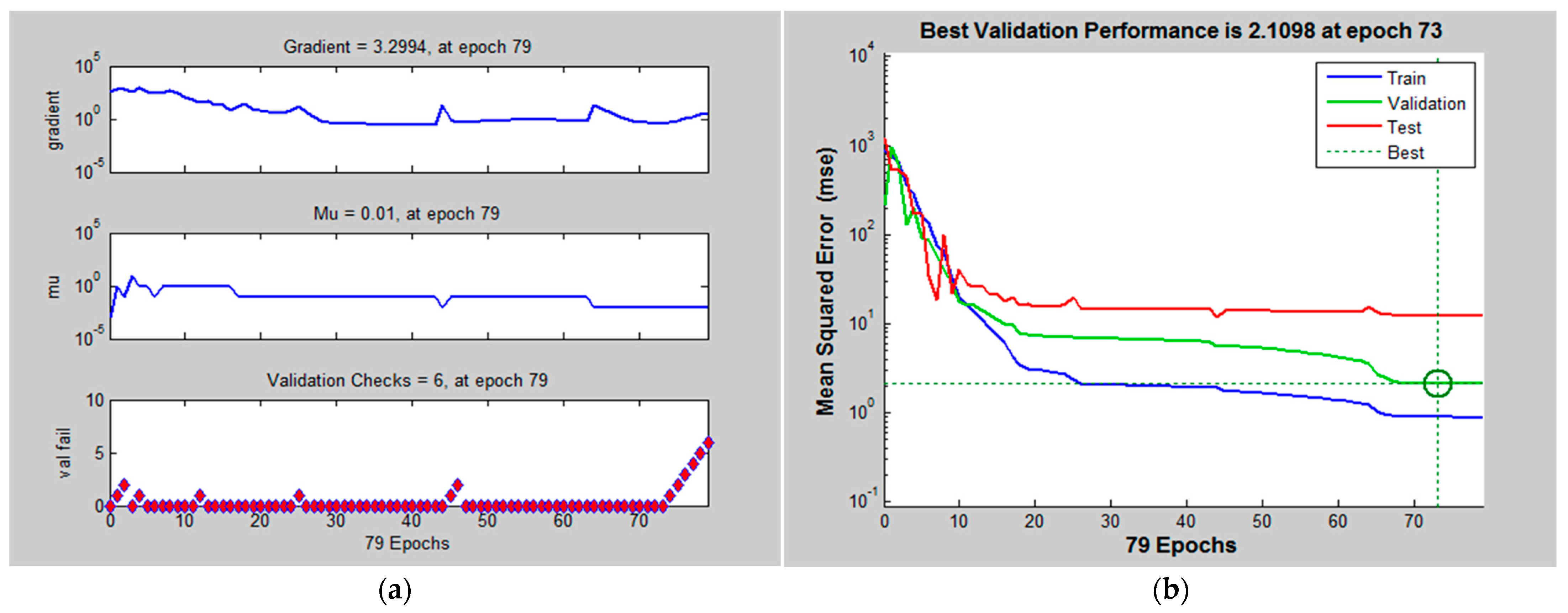
| Max. Iteration * | 8 | 55 | 79 | 54 | 69 | 56 | |
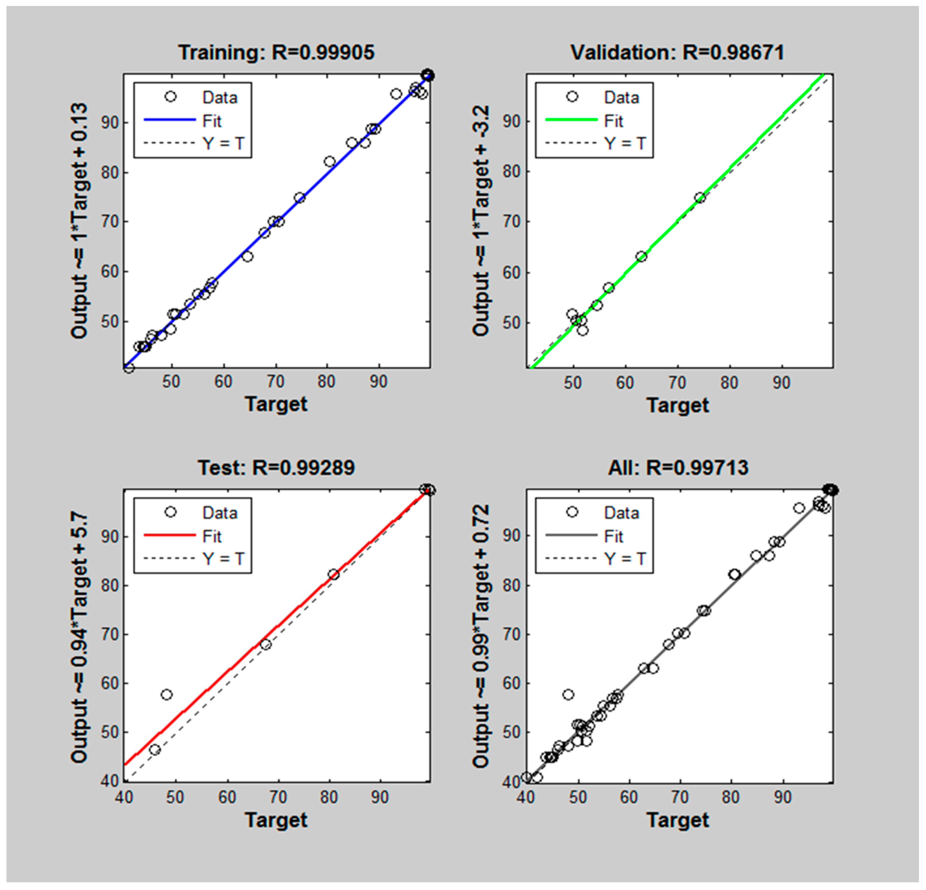
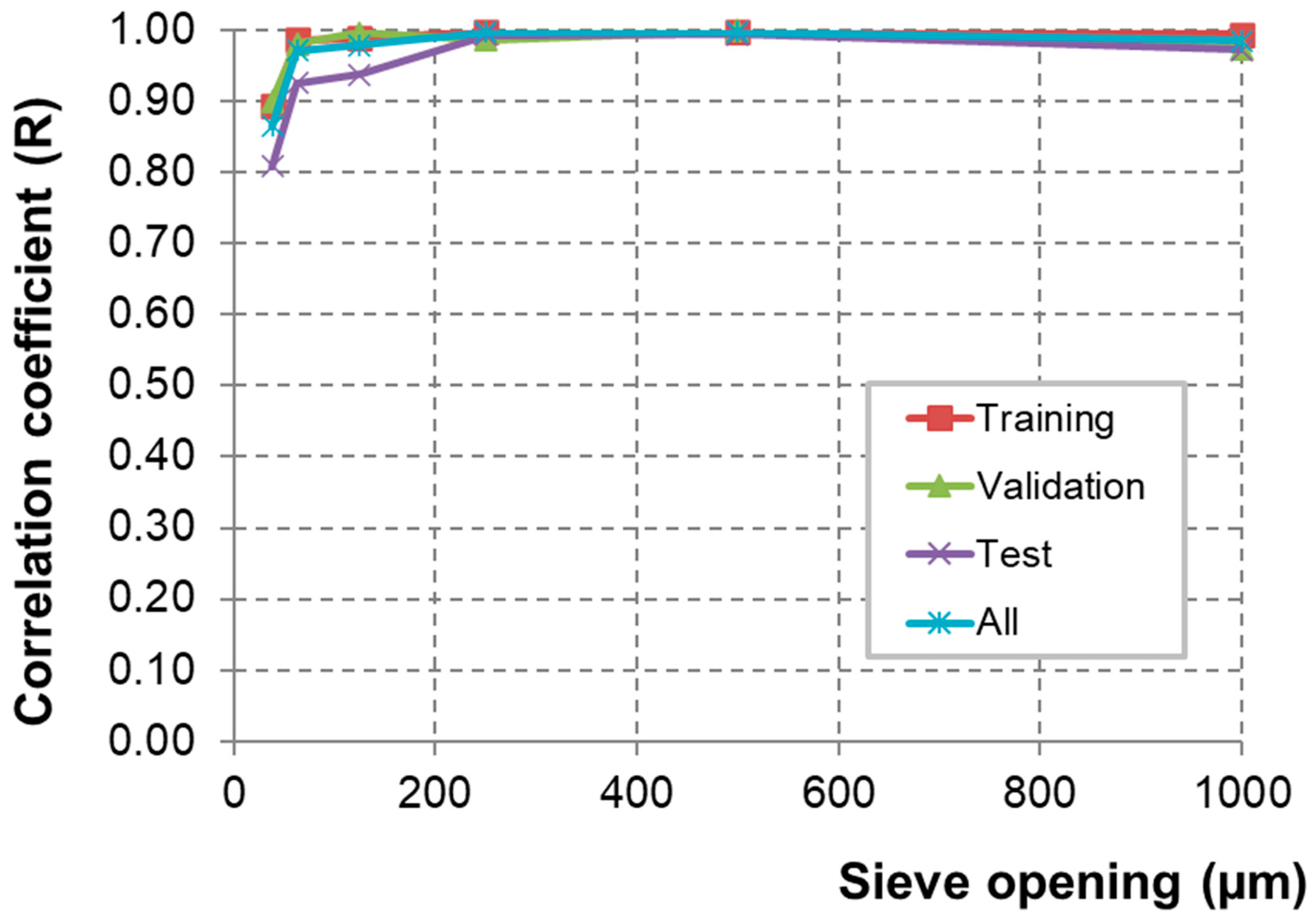
| Correlation coefficient (R) | Training | 0.994 | 0.997 | 0.999 | 0.998 | 0.987 | 0.893 |
| Validation | 0.974 | 0.999 | 0.987 | 0.996 | 0.981 | 0.901 | |
| Test | 0.973 | 0.995 | 0.993 | 0.938 | 0.926 | 0.809 | |
Publisher’s Note: MDPI stays neutral with regard to jurisdictional claims in published maps and institutional affiliations. |
© 2022 by the authors. Licensee MDPI, Basel, Switzerland. This article is an open access article distributed under the terms and conditions of the Creative Commons Attribution (CC BY) license (https://creativecommons.org/licenses/by/4.0/).
Share and Cite
Otsuki, A.; Jang, H. Prediction of Particle Size Distribution of Mill Products Using Artificial Neural Networks. ChemEngineering 2022, 6, 92. https://doi.org/10.3390/chemengineering6060092
Otsuki A, Jang H. Prediction of Particle Size Distribution of Mill Products Using Artificial Neural Networks. ChemEngineering. 2022; 6(6):92. https://doi.org/10.3390/chemengineering6060092
Chicago/Turabian StyleOtsuki, Akira, and Hyongdoo Jang. 2022. "Prediction of Particle Size Distribution of Mill Products Using Artificial Neural Networks" ChemEngineering 6, no. 6: 92. https://doi.org/10.3390/chemengineering6060092