

Recent Progress in the Viscosity Modeling of Concentrated Suspensions of Unimodal Hard Spheres
Abstract
:1. Introduction
2. Theoretical Background
2.1. Dilute Suspensions of Hard Spheres
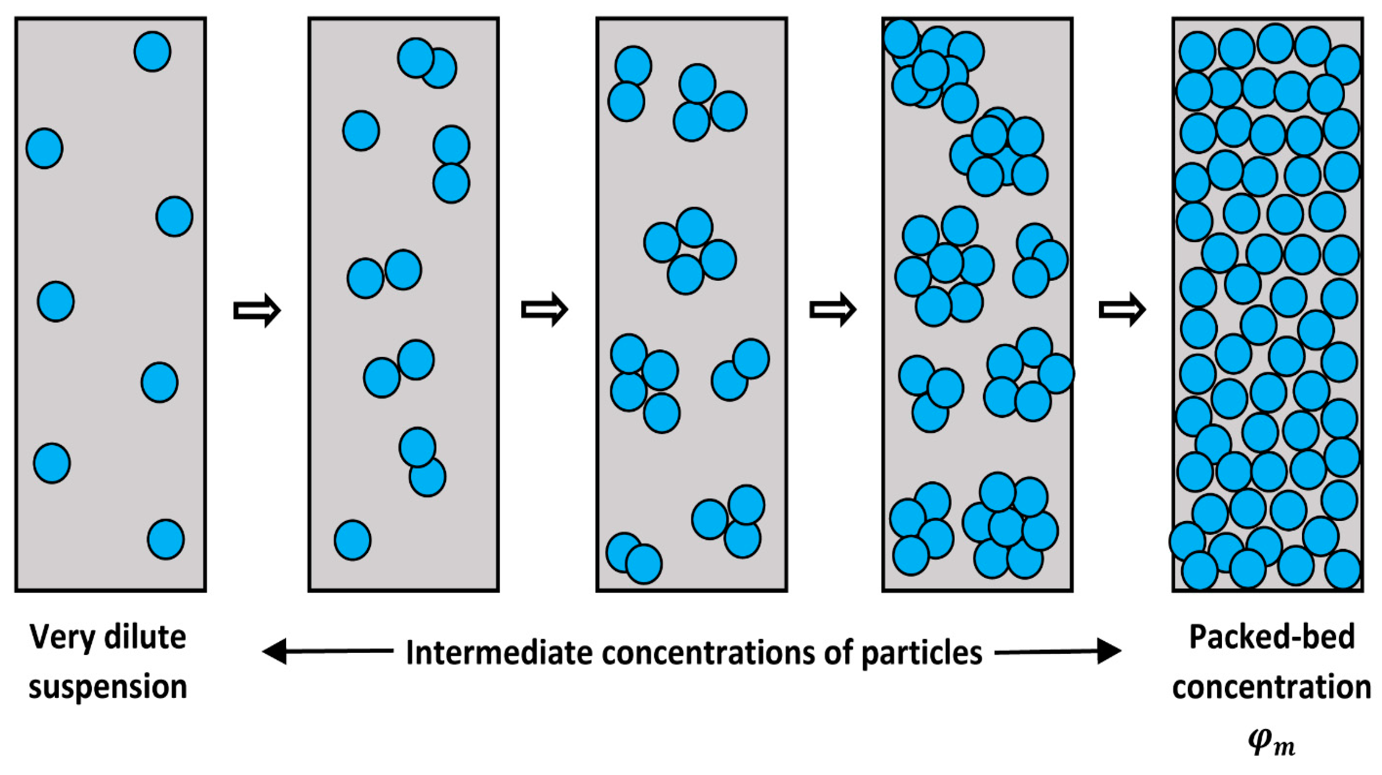
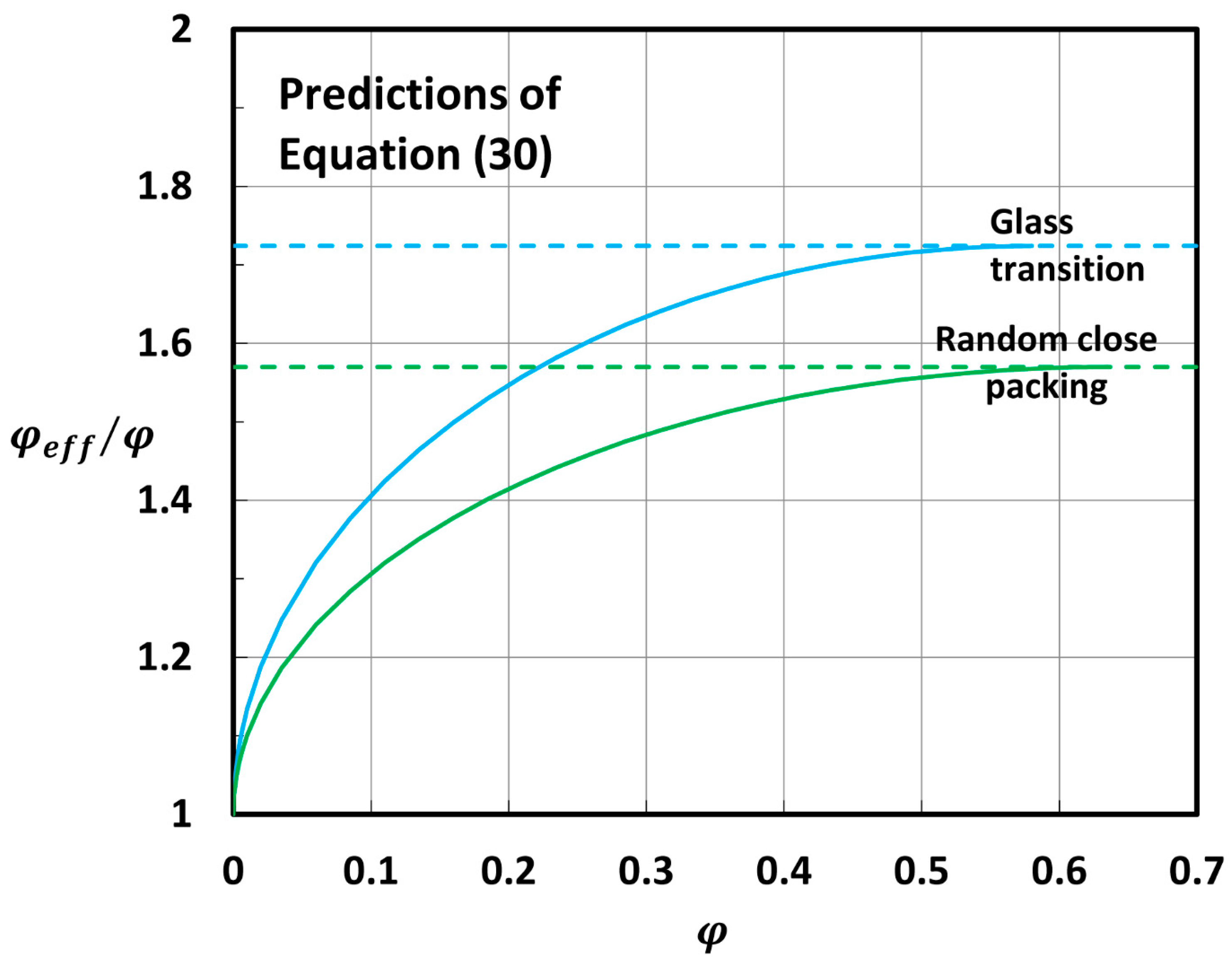
2.2. Concentrated Suspensions of Hard Spheres
3. Recent Progress in the Viscosity Modeling of Concentrated Suspensions
3.1. Cheng et al. Model (2002)
3.2. Mendoza and Santamaria-Holek Model (2009)
3.3. Brouwers Model (2010)
3.4. Faroughi–Huber Model (2015)
3.5. Pal Model (2015)
3.6. Pal Model (2017)
3.7. Pal Model (2020)
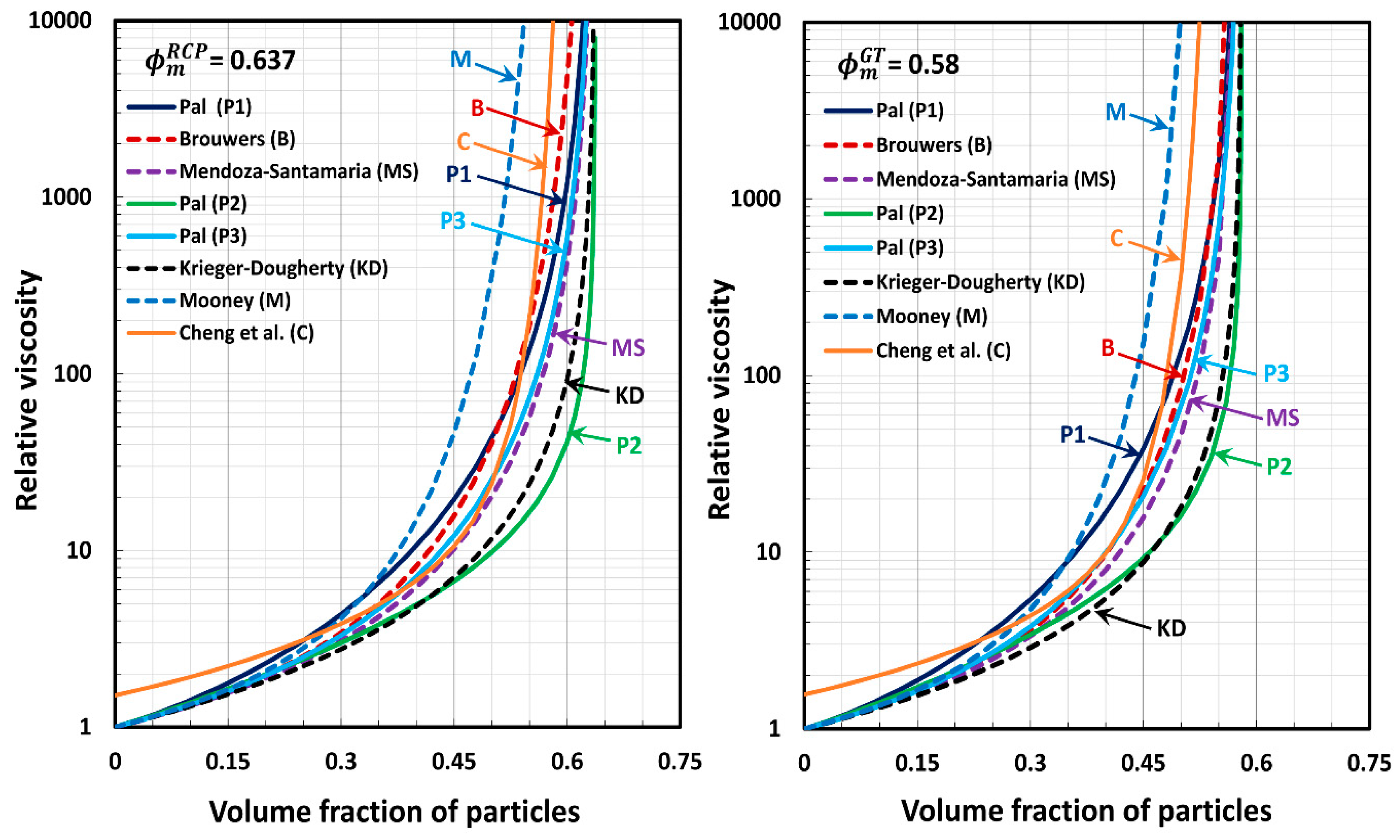
4. Comparisons of Model Predictions
- The Mooney model (M) generally predicts the highest values of relative viscosities.
- Pal model P2 generally predicts the lowest values of relative viscosities.
- The Krieger–Dougherty model (KD) and Pal model P2 predict similar values of relative viscosities.
- The Mendoza and Santamaria-Holek model (MS) generally predicts relative viscosities lower than that of Pal model P3.
- The Cheng et al. (C) model predicts unrealistically high values of relative viscosities when . Also, the relative viscosity is greater than unity at
- For large values of particle volume fractions , the predictions of the models are generally in the following order: .
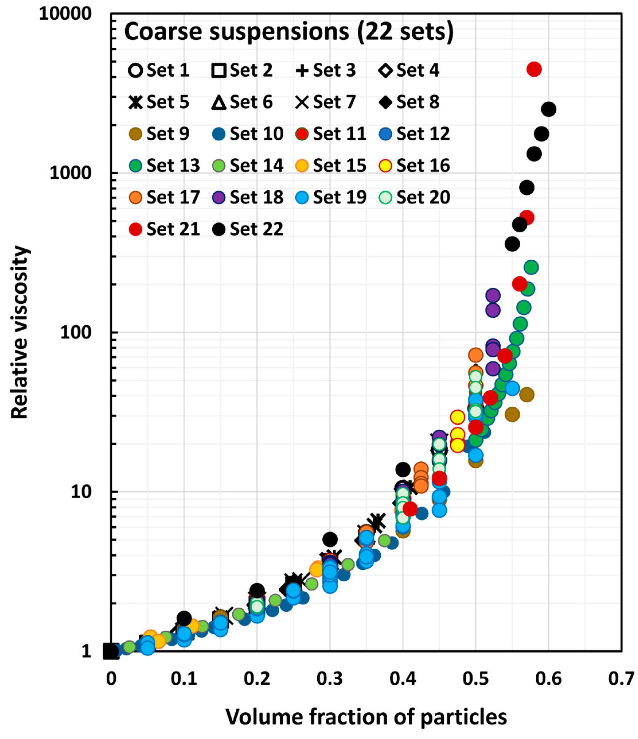
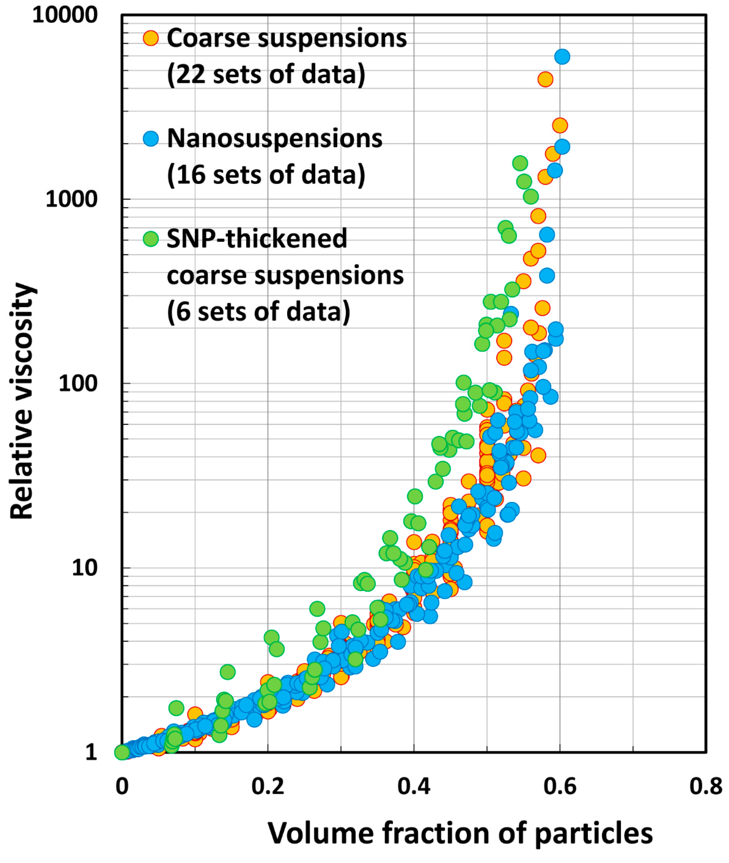
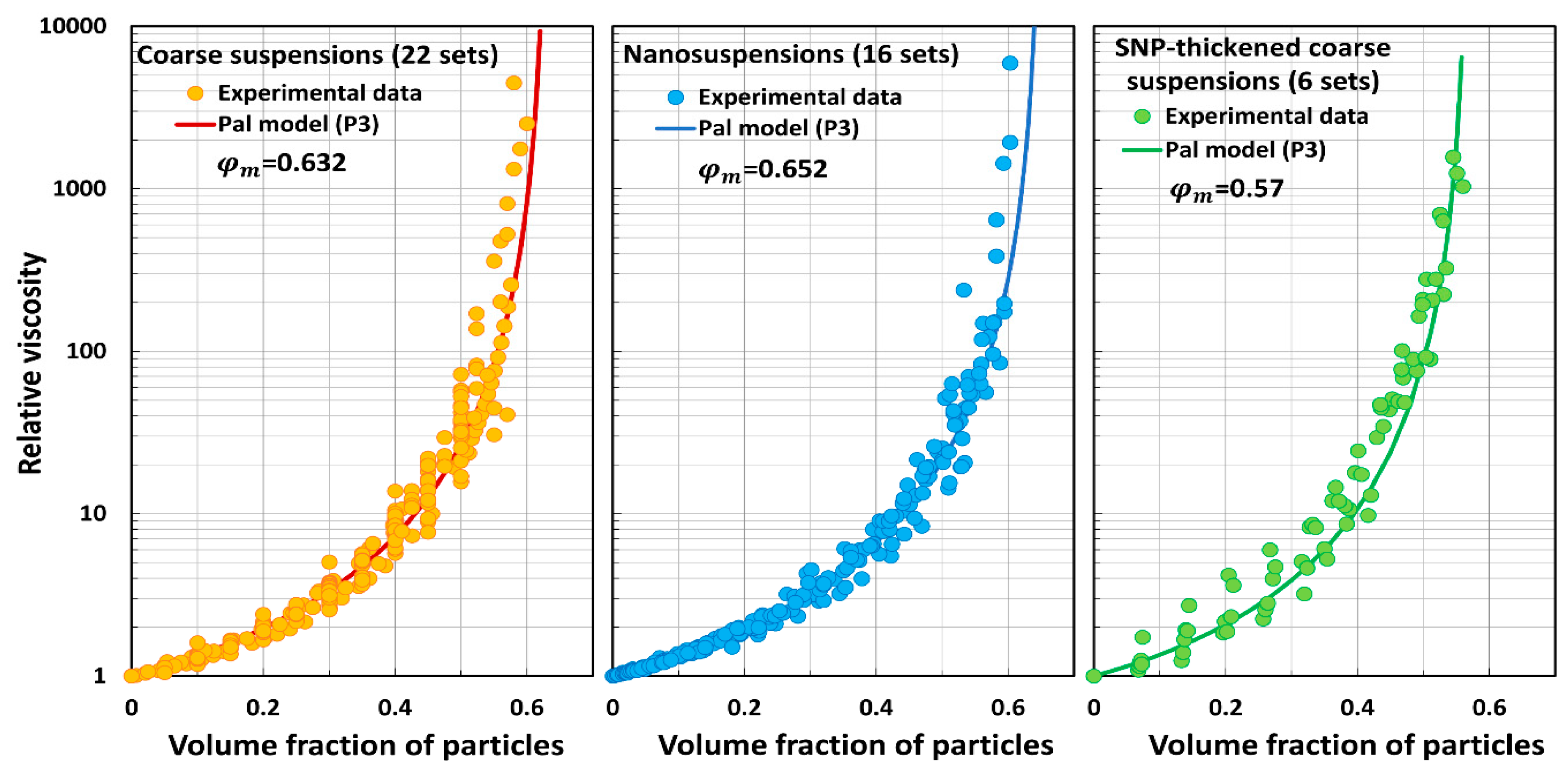
5. Comparisons of Model Predictions with Experimental Data
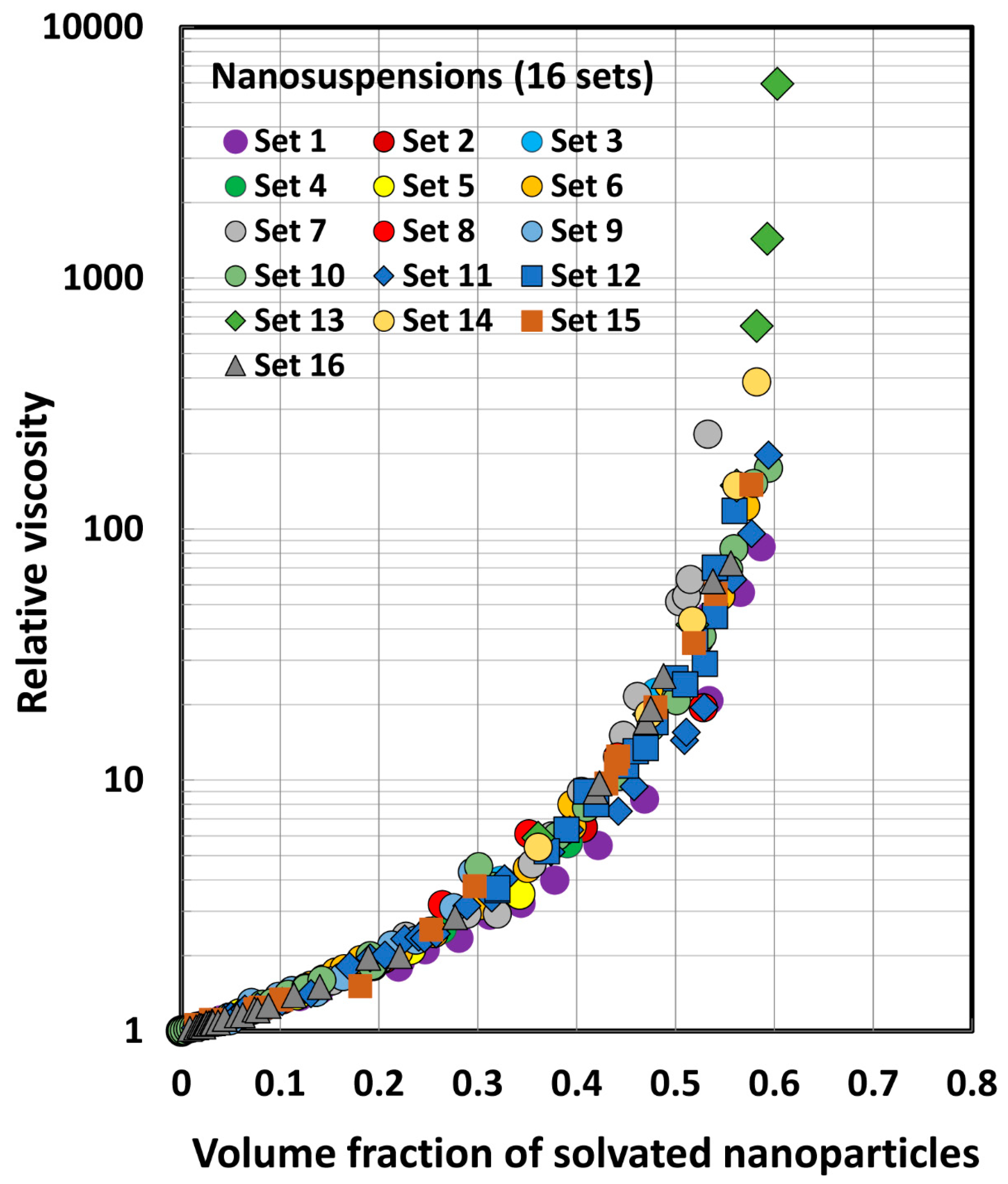
5.1. Experimental Data
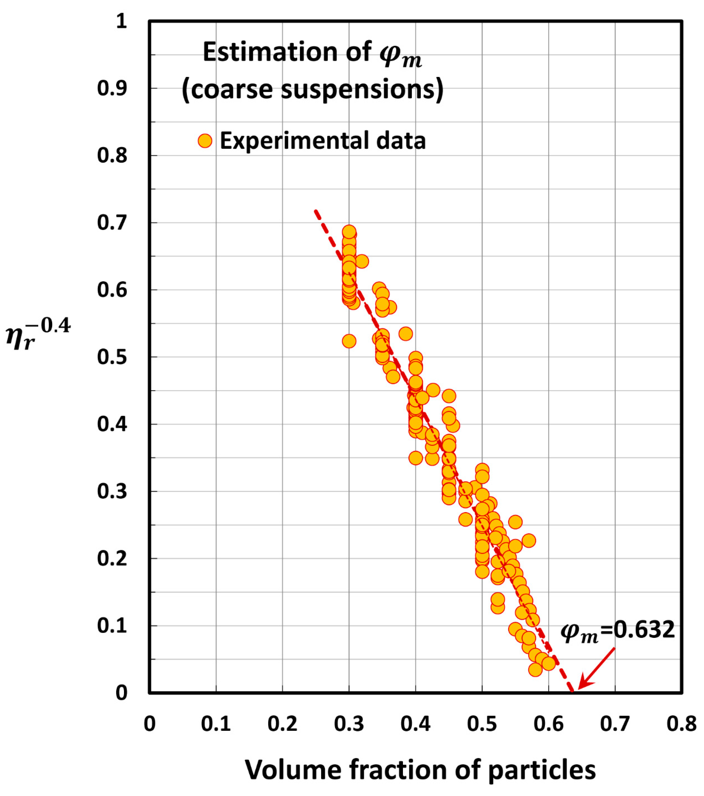
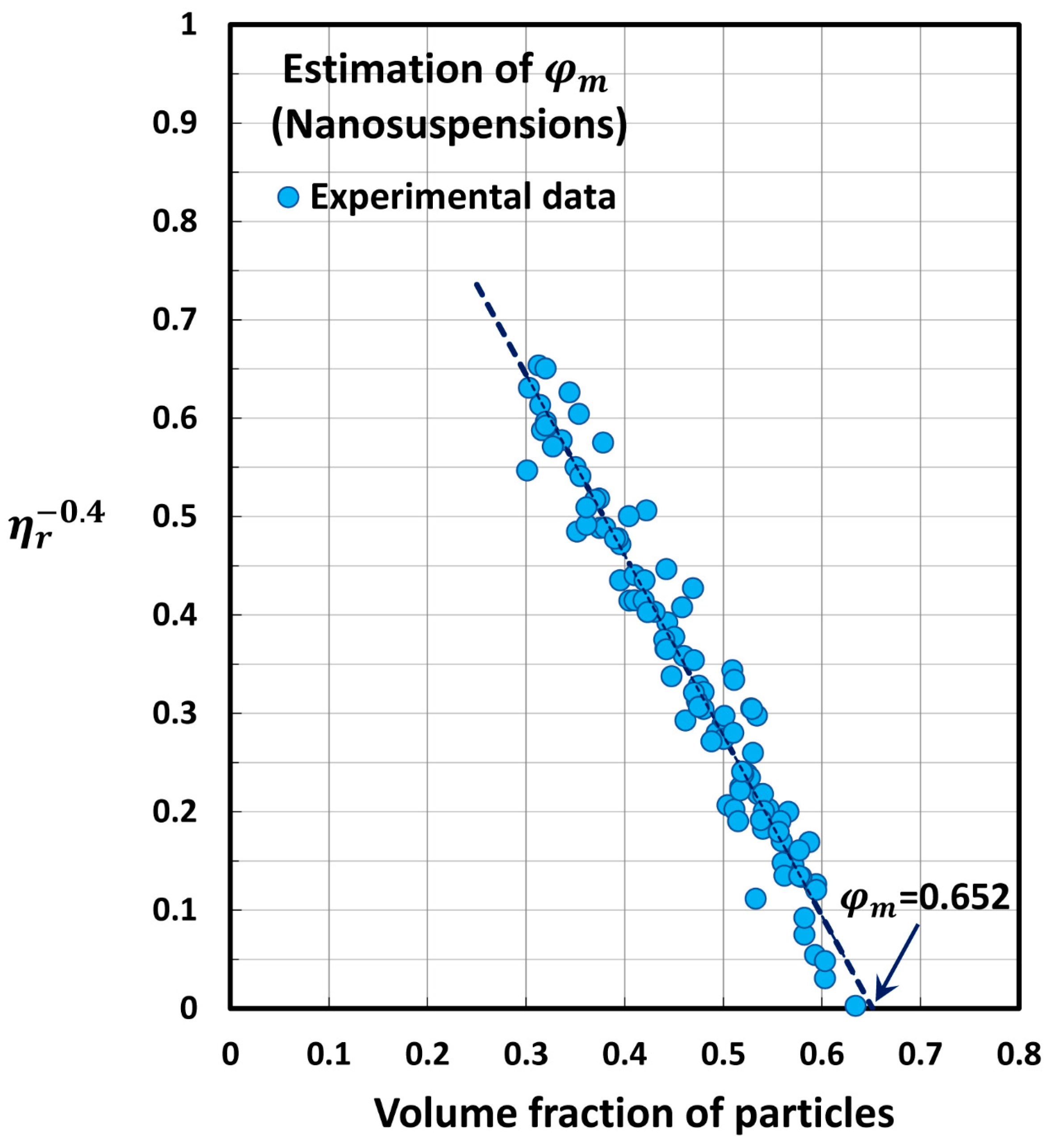
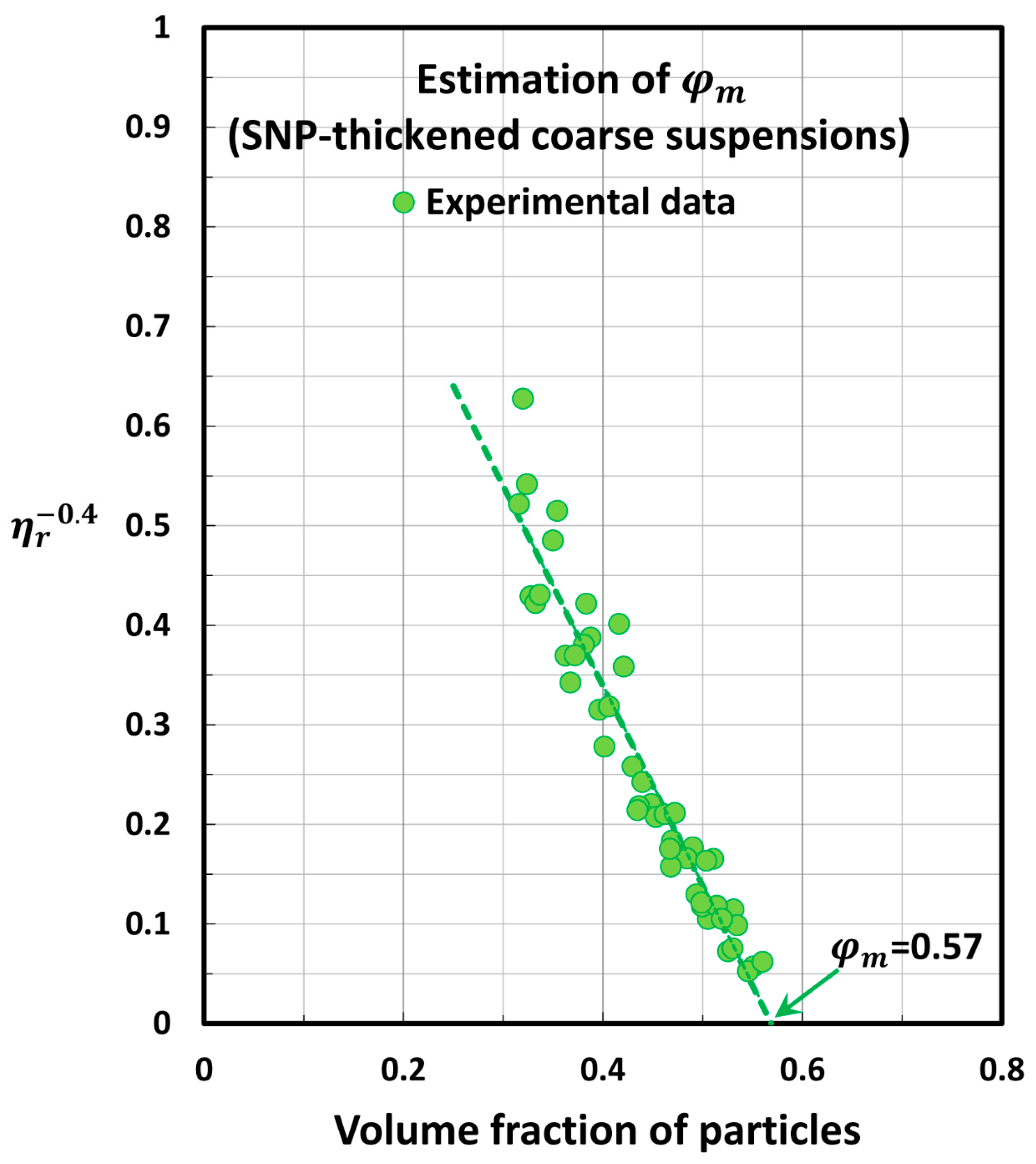
5.2. Estimation of Maximum Packing Volume Fraction of Suspensions
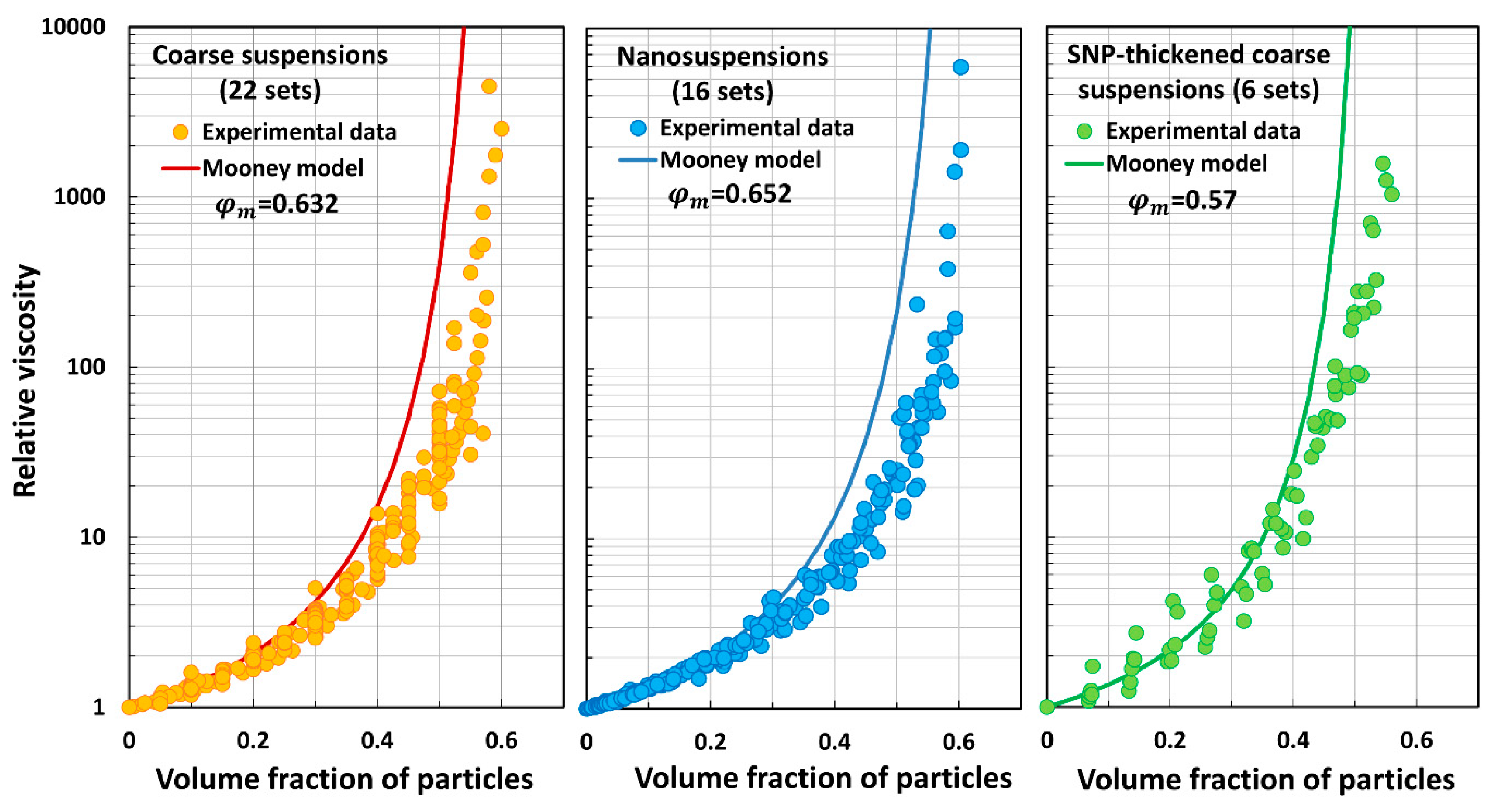
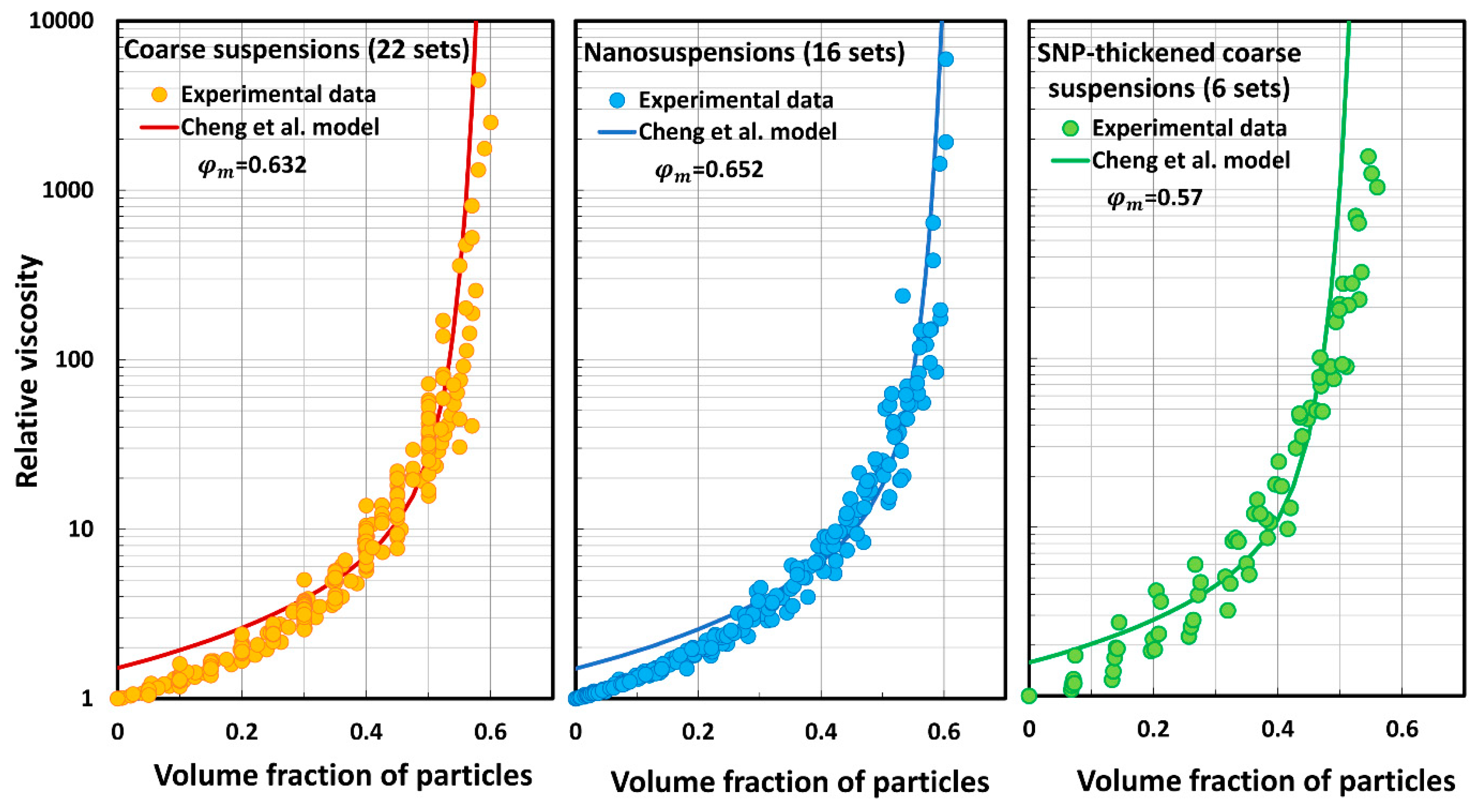
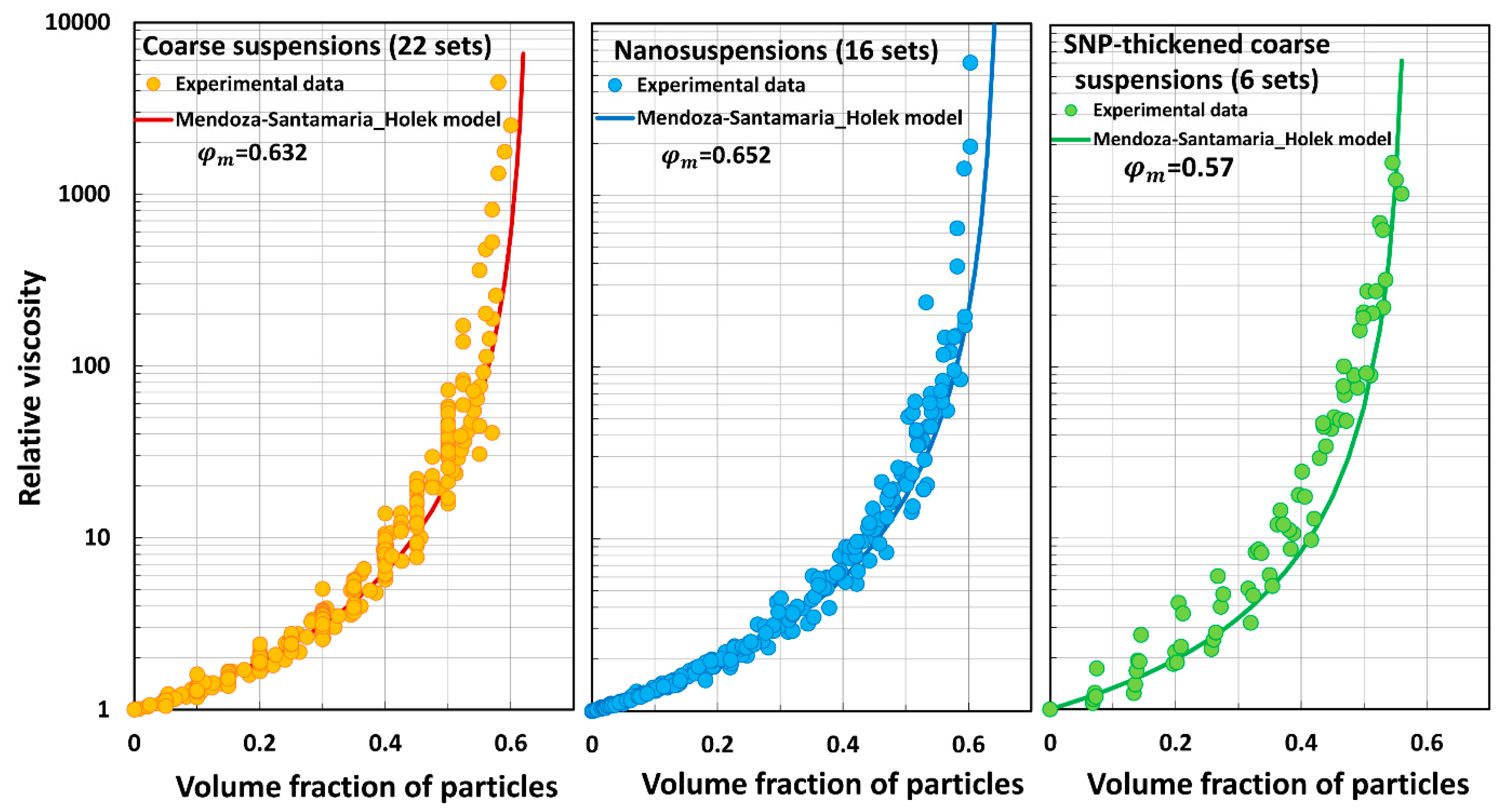
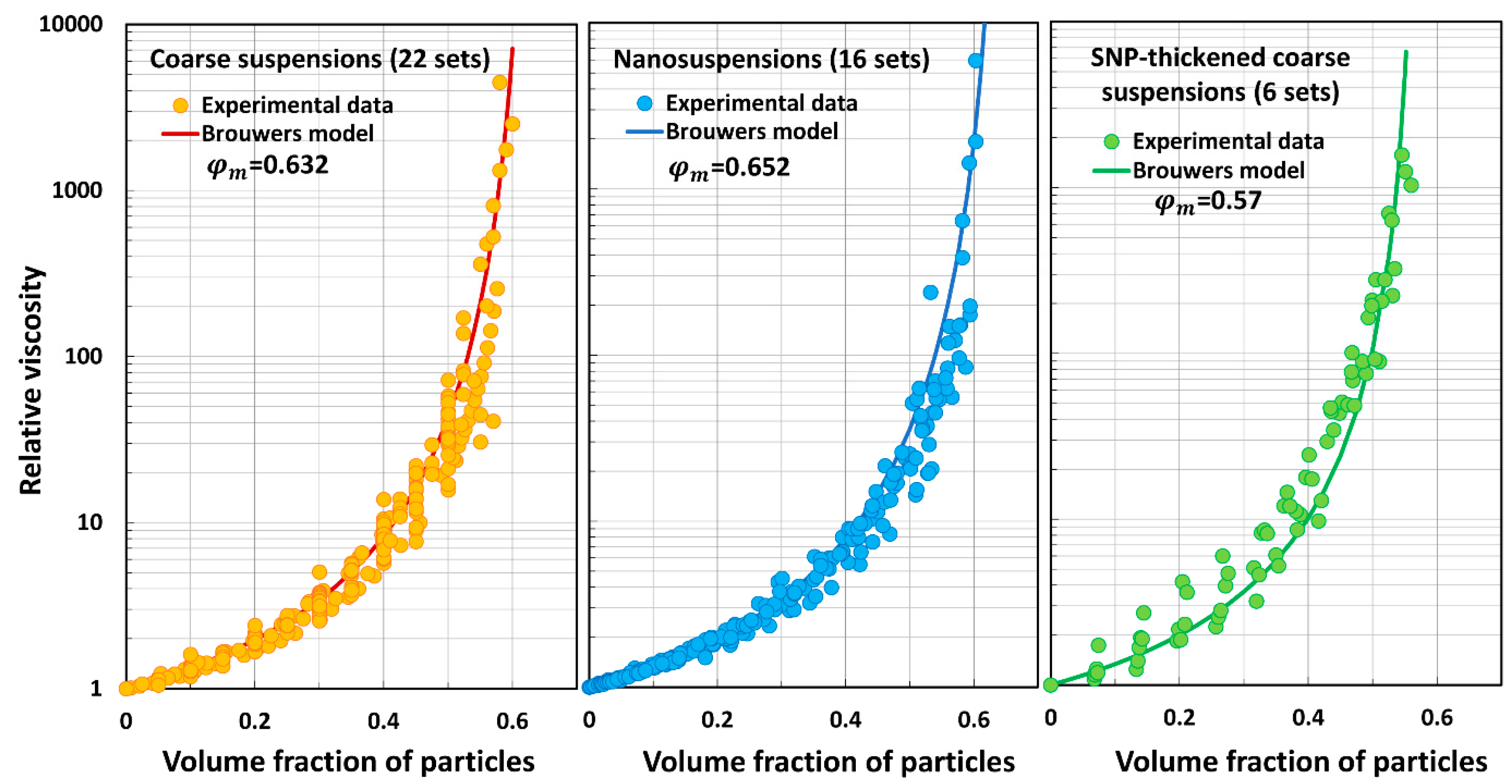
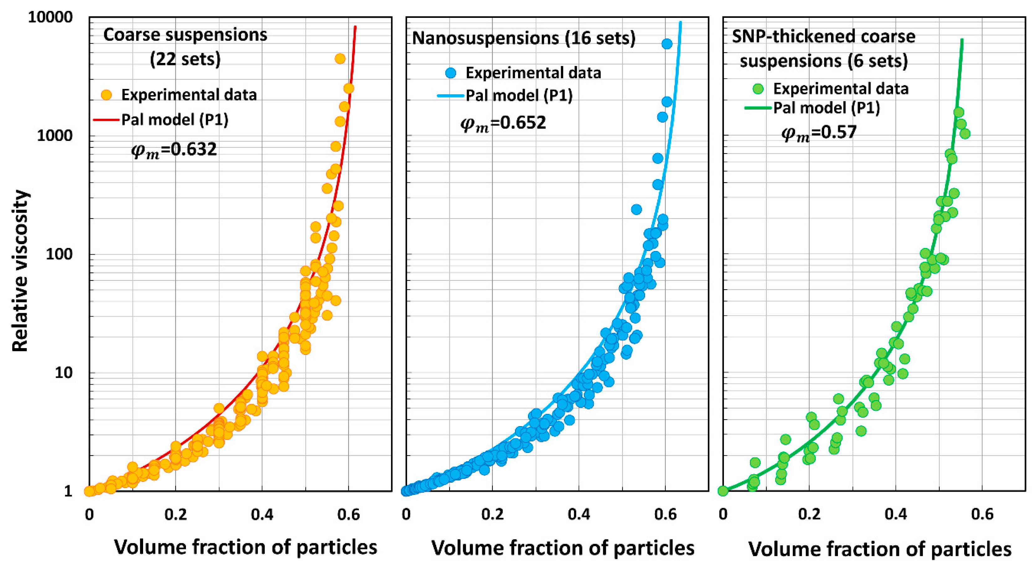
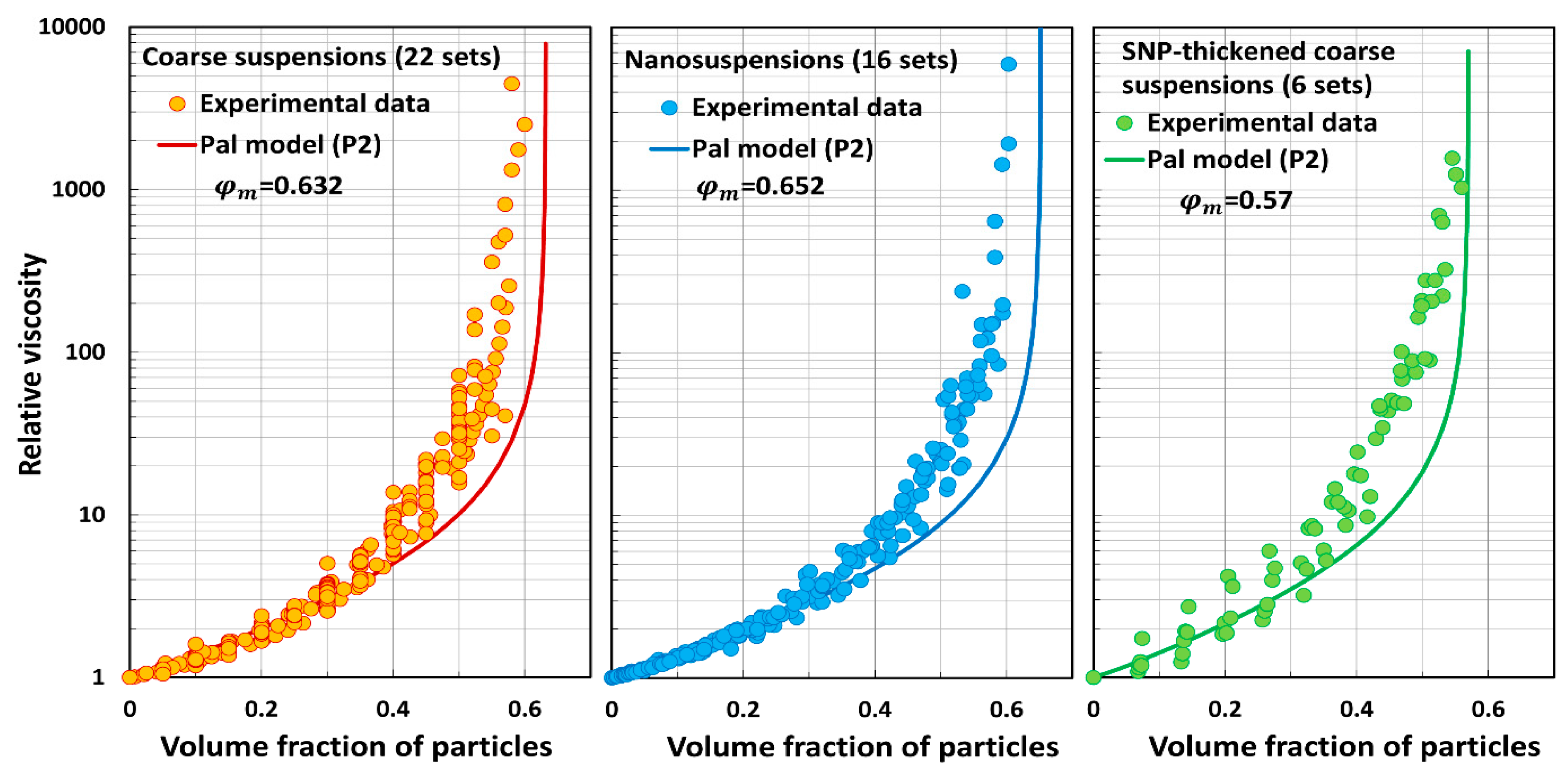
5.3. Model Predictions Versus Experimental Data
- The Mooney model (M) overpredicts the relative viscosity of suspensions.
- The Krieger–Dougherty model (KD) underpredicts the relative viscosity of suspensions.
- The Cheng et al. model (C) overpredicts the relative viscosity at low and high particle concentrations.
- The Mendoza and Santamaria-Holek model (MS) underpredicts the relative viscosity of suspensions.
- The Brouwers model (B) overpredicts the relative viscosity of suspensions.
- Pal model P1 overpredicts the relative viscosity of suspensions.
- Pal model P2 underpredicts the relative viscosity of suspensions.
- Pal model P3 predictions are close to experimental values.
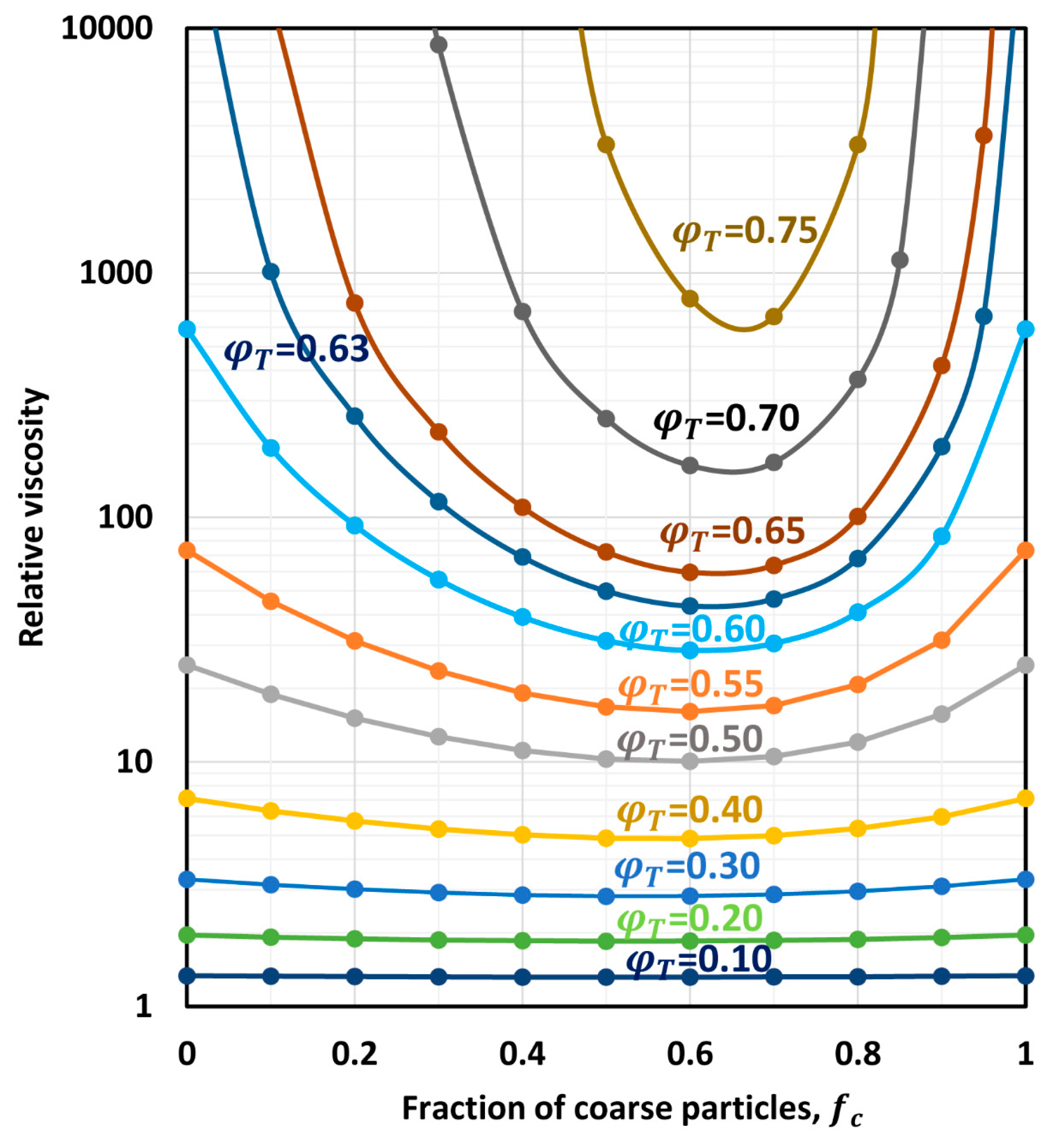
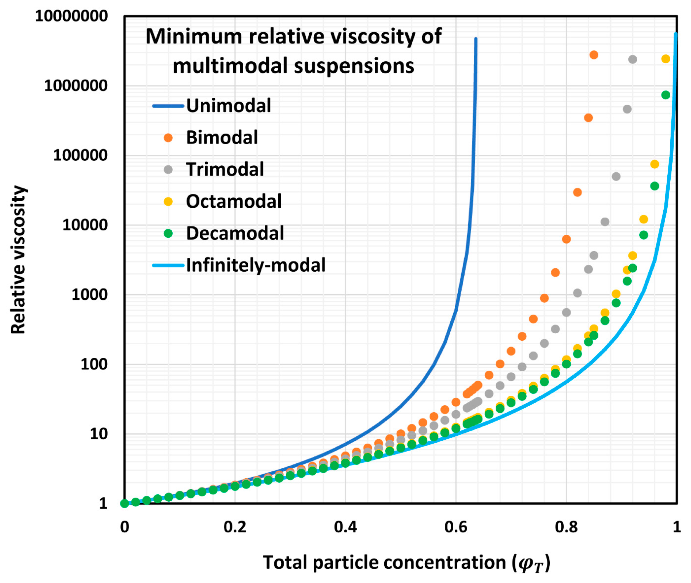
6. Simulation of the Viscous Behavior of Concentrated Multimodal Suspensions
6.1. Relative Viscosity of Bimodal Suspensions
6.2. Minimum Relative Viscosity of Multimodal Suspensions
6.3. Composition of Multimodal Suspensions at Minimum Relative Viscosity
7. Conclusions
Funding
Data Availability Statement
Conflicts of Interest
Nomenclature
| Greek Symbols | |
| Unit tensor | |
| Viscosity | |
| Viscosity of matrix phase (suspending medium) | |
| Relative viscosity | |
| High-frequency relative viscosity | |
| Experimental value of relative viscosity | |
| Relative viscosity predicted by the model | |
| Non-hydrodynamic contribution to relative viscosity (see Equation (16)) | |
| Bulk stress tensor | |
| Volume fraction of particles | |
| Effective volume fraction of particles | |
| Volume fraction of ith set of particles in a multimodal suspension, defined in Equations (48) and (49) | |
| Maximum packing volume fraction of particles where the viscosity of suspension diverges | |
| Volume fraction of nth set of particles in a multimodal suspension, defined in Equations (48) and (49) | |
| Volume fraction of different-size particles in a multimodal suspension corresponding to minimum relative viscosity of suspension (see Equation (61)) | |
| Total volume fraction of particles in a multimodal suspension, defined in Equation (51) | |
| Self-crowding parameter, defined in Equation (28) | |
| Latin Symbols | |
| a | Constant in Equation (42) |
| APRE | Average percentage relative error |
| b | Constant in Equation (42) |
| c | Self-crowding parameter (see Equation (22)) |
| Bulk rate of strain tensor | |
| Rate of strain tensor far away from the particle | |
| Fraction (volume basis) of coarse particles in a bimodal or trimodal mixture of particles | |
| Fraction (volume basis) of fine particles in a bimodal or trimodal mixture of particles | |
| Fraction (volume basis) of medium-sized particles in a trimodal mixture of particles | |
| GT | Glass transition point |
| H | Relative viscosity function |
| k | Aggregation coefficient (see Equation (42)) |
| n | Number of data points or nth set of particles in a multimodal suspension |
| N | Number of different-size particle fractions in a multimodal suspension, same as modality |
| P | Pressure |
| R | Radius of particle |
| RCP | Random close packing |
| Dipole strength of a single particle in an infinite matrix | |
| Volume of smallest-size particles in a multimodal suspension | |
| Volume of ith set of particles in a multimodal suspension | |
| Volume of suspending medium of a multimodal suspension | |
| Volume of nth set of particles in a multimodal suspension | |
| Volume of largest-size particles in a multimodal suspension | |
References
- Pal, R. Rheology of Particulate Dispersions and Composites; CRC Press: Boca Raton, FL, USA, 2007. [Google Scholar]
- Pal, R. Electromagnetic, Mechanical, and Transport Properties of Composite Materials; CRC Press: Boca Raton, FL, USA, 2015. [Google Scholar]
- Stickel, J.J.; Powell, R.L. Fluid mechanics and rheology of dense suspensions. Annu. Rev. Fluid Mech. 2005, 37, 127–149. [Google Scholar] [CrossRef]
- Denn, M.M.; Morris, J.F. Rheology of non-Brownian suspensions. Annu. Rev. Chem. Biomol. Eng. 2014, 5, 203–228. [Google Scholar] [CrossRef] [PubMed]
- Guazzelli, E.; Pouliquen, O. Rheology of dense granular suspensions. J. Fluid. Mech. 2018, 852, P1. [Google Scholar] [CrossRef] [Green Version]
- Tadros, T.F. Suspension Concentrates: Preparation, Stability and Industrial Applications; De Gruyter: Berlin, Germany; Boston, MA, USA, 2017. [Google Scholar]
- Schramm, L.L. Emulsions, Foams, Suspensions, and Aerosols: Microscience and Applications; Wiley-VCH Verlag: Weinheim, Germany, 2014. [Google Scholar]
- Kulshreshtha, A.; Wall, M. Pharmaceutical Suspensions: From Formulation Development to Manufacturing; Springer: London, UK, 2010. [Google Scholar]
- Halloran, J.W.; Tomeckova, V. Flow behavior of polymerizable ceramic suspensions as function of ceramic volume fraction and temperature. J. Eur. Ceram. Soc. 2011, 31, 2535–2542. [Google Scholar]
- Camargo, I.L.; Morais, M.M.; Fortulan, C.A.; Branciforti, M.C. A review on the rheological behavior and formulations of ceramic suspensions for vat polymerization. Ceram. Int. 2021, 47, 11906–11921. [Google Scholar] [CrossRef]
- Zhou, W.; Li, D.; Wang, H. A novel aqueous ceramic suspension for ceramic stereolithography. Rapid Prototyp. J. 2010, 16, 29–35. [Google Scholar] [CrossRef]
- Pal, R. Modeling the viscosity of concentrated nanoemulsions and nanosuspensions. Fluids 2016, 1, 11. [Google Scholar] [CrossRef] [Green Version]
- Einstein, A. Eine neue Bestimmung der Molekuldimension. Ann. Phys. 1906, 19, 289–306. [Google Scholar] [CrossRef] [Green Version]
- Einstein, A. Berichtigung zumeiner Arbeit: Eine neue Bestimmung derMolekuldimension. Ann. Phys. 1911, 34, 591–592. [Google Scholar] [CrossRef] [Green Version]
- Batchelor, G.K. Effect of Brownian motion on bulk stress in a suspension of spherical particles. J. Fluid Mech. 1977, 83, 97–117. [Google Scholar] [CrossRef]
- Brady, J.F.; Bossis, G. Stokesian dynamics. Ann. Rev. Fluid Mech. 1988, 20, 111–157. [Google Scholar] [CrossRef]
- Ladd, A.J.C. Hydrodynamic transport coefficients of random dispersions of hard spheres. J. Chem. Phys. 1990, 93, 3483–3494. [Google Scholar] [CrossRef]
- Wang, G.; Fiore, A.M.; Swan, J.W. On the viscosity of adhesive hard sphere dispersions: Critical scaling and the role of rigid contacts. J. Rheol. 2019, 63, 229–245. [Google Scholar] [CrossRef]
- Taylor, G.I. The viscosity of a fluid containing small drops of another liquid. Proc. R. Soc. Lond. A 1932, 138, 41–48. [Google Scholar]
- Vand, V. Viscosity of solutions and suspensions. 1. Theory. J. Phys. Colloid Chem. 1948, 52, 277–299. [Google Scholar] [CrossRef]
- Vand, V. Viscosity of solutions and suspensions. II. Experimental determination of the viscosity-concentration function of spherical inclusions. J. Phys. Colloid Chem. 1948, 52, 300–314. [Google Scholar] [CrossRef]
- Ward, S.G.; Whitmore, R.L. Studies of the viscosity and sedimentation of suspensions Part 1.—The viscosity of suspension of spherical particles. Br. J. Appl. Phys. 1950, 1, 286–290. [Google Scholar] [CrossRef]
- Saito, N. Concentration dependence of the viscosity of high polymer solutions. J. Phys. Soc. 1950, 5, 4–8. [Google Scholar] [CrossRef]
- Mooney, M. The viscosity of a concentrated suspension of spherical particles. J. Colloid Sci. 1951, 6, 162–170. [Google Scholar] [CrossRef]
- Roscoe, R. The viscosity of suspensions of rigid spheres. Br. J. Appl. Phys. 1952, 3, 267–269. [Google Scholar] [CrossRef]
- Brinkman, H.C. The viscosity of concentrated suspensions and solutions. J. Chem. Phys. 1952, 20, 571–581. [Google Scholar] [CrossRef]
- Simha, R. A treatment of the viscosity of concentrated suspensions. J. Appl. Phys. 1952, 23, 1020–1024. [Google Scholar] [CrossRef]
- Oldroyd, J.G. The elastic and viscous properties of emulsions and suspensions. Proc. R. Soc. Lond. A 1953, 218, 122–132. [Google Scholar]
- Manley, R.S.J.; Mason, S.G. The viscosity of suspensions of spheres: A note on the particle interaction coefficient. Can. J. Chem. 1954, 32, 763–767. [Google Scholar] [CrossRef]
- Van der Waarden, M. Viscosity and electroviscous effect of emulsions. J. Colloid Sci. 1954, 9, 215–222. [Google Scholar] [CrossRef]
- Maron, S.H.; Pierce, P.E. Application of Ree-Eyring generalized flow theory to suspensions of spherical particles. J. Colloid Sci. 1956, 11, 80–95. [Google Scholar] [CrossRef]
- Happel, J. Viscosity of suspensions of uniform spheres. J. Appl. Phys. 1957, 28, 1288–1292. [Google Scholar] [CrossRef]
- Ting, A.P.; Luebbers, R.H. Viscosity of suspensions of spherical and other isodimensional particles in liquids. AIChE J. 1957, 3, 111–116. [Google Scholar] [CrossRef] [Green Version]
- Krieger, I.M.; Dougherty, T.J. Mechanism for non-Newtonian flow in suspensions of rigid particles. Trans. Soc. Rheol. 1959, 3, 137–152. [Google Scholar] [CrossRef]
- Rutgers, R. Relative viscosity of suspensions of rigid spheres in Newtonian liquids. Rheol. Acta 1962, 2, 202–210. [Google Scholar] [CrossRef]
- Thomas, D.G. Transport characteristics of suspensions: VIII. A note on the viscosity of Newtonian suspensions of uniform spherical particles. J. Colloid Sci. 1965, 20, 267–277. [Google Scholar]
- Frankel, N.A.; Acrivos, A. On the viscosity of a concentrated suspension of solid spheres. Chem. Eng. Sci. 1967, 22, 847–853. [Google Scholar] [CrossRef]
- Chong, J.S.; Christiansen, E.B.; Baer, A.D. Rheology of concentrated suspensions. Trans. Soc. Rheol. 1968, 12, 281–301. [Google Scholar] [CrossRef]
- Lewis, T.B.; Nielsen, L.E. Viscosity of dispersed and aggregated suspensions of spheres. J. Rheol. 1968, 12, 421–443. [Google Scholar] [CrossRef]
- Batchelor, G.K.; Green, J.T. The determination of the bulk stress in a suspension of spherical particles to order c2. J. Fluid Mech. 1972, 56, 401–427. [Google Scholar] [CrossRef]
- Yaron, I.; Gal-Or, B. On viscous flow and effective viscosity of concentrated suspensions and emulsions. Rheol. Acta 1972, 11, 241–252. [Google Scholar] [CrossRef]
- Smith, J.H. Rheology of Concentrated Suspensions of Spheres. Ph.D. Thesis, California Institute of Technology, Pasadena, CA, USA, 1972. [Google Scholar]
- Jeffrey, D.J.; Acrivos, A. The rheological properties of suspensions of rigid particles. AIChE J. 1976, 22, 417–432. [Google Scholar] [CrossRef]
- Quemada, D. Rheology of concentrated disperse systems and minimum energy dissipation principle: 1. Viscosity-concentration relationship. Rheol. Acta 1977, 16, 82–94. [Google Scholar] [CrossRef]
- Graham, A.L. On the viscosity of suspensions of solid spheres. Appl. Sci. Res. 1981, 37, 275–286. [Google Scholar] [CrossRef]
- Graham, A.L.; Bird, R.B. Particle clusters in concentrated suspensions. 1. Experimental observations of particle clusters. Ind. Eng. Chem. Fundam. 1984, 23, 406–410. [Google Scholar] [CrossRef]
- Metzner, A.B. Rheology of Suspensions in Polymeric Liquids. J. Rheol. 1985, 29, 739–775. [Google Scholar] [CrossRef]
- Poslinski, A.J.; Ryan, M.E.; Gupta, R.K.; Seshadri, S.G.; Frechette, F.J. Rheological behavior of filled polymeric systems I. Yield stress and shear-thinning effects. J. Rheol. 1988, 32, 703–735. [Google Scholar] [CrossRef]
- Poslinski, A.J.; Ryan, M.E.; Gupta, R.K.; Seshadri, S.G.; Frechette, F.J. Rheological behavior of filled polymeric systems II. The effect of a bimodal size distribution of particulates. J. Rheol. 1988, 32, 751–771. [Google Scholar]
- Pal, R.; Rhodes, E. Viscosity/concentration relationships for emulsions. J. Rheol. 1989, 33, 1021–1045. [Google Scholar] [CrossRef]
- Park, M.; Gandhi, K.; Sun, L.; Salovey, R. Model-filled polymers. III: Rheological behavior of polystyrene containing cross-linked polystyrene beads. Polym. Sci. Eng. 1990, 30, 1158–1164. [Google Scholar]
- Jones, A.A.R.; Leary, B.; Boger, D.V. The rheology of a concentrated colloidal suspension of hard spheres. J. Colloid Interface Sci. 1991, 147, 479–495. [Google Scholar] [CrossRef]
- Jones, A.A.R.; Leary, B.; Boger, D.V. The rheology of a sterically stabilized suspension at high concentration. J. Colloid Interface Sci. 1992, 150, 84–96. [Google Scholar] [CrossRef]
- Ilic, V.; Phan-Thien, N. Viscosity of concentrated suspensions of spheres. Rheol. Acta 1994, 33, 283–291. [Google Scholar] [CrossRef]
- Pal, R. Rheology of emulsions containing polymeric liquids. In Encyclopedia of Emulsion Technology; Chapter, 3, Becher, P., Eds.; Dekker: New York, NY, USA, 1996; Volume 4. [Google Scholar]
- Weiss, A.; Dingenouts, N.; Ballaquff, M.; Senf, H.; Richtering, W. Comparison of the effective radius of sterically stabilized latex particles determined by small angle X-ray scattering and by zero shear viscosity. Langmuir 1998, 14, 5083–5087. [Google Scholar] [CrossRef]
- Pal, R. Linear viscoelastic behavior of multiphase dispersions. J. Colloid Interface Sci. 2000, 232, 50–63. [Google Scholar] [CrossRef]
- Zarraga, I.E.; Hill, D.A.; Leighton, D.T. The characterization of the total stress of concentrated suspensions of noncolloidal spheres in Newtonian fluids. J. Rheol. 2000, 44, 185–220. [Google Scholar] [CrossRef]
- Pal, R. Evaluation of theoretical viscosity models for concentrated emulsions at low capillary numbers. Chem. Eng. J. 2001, 81, 15–21. [Google Scholar] [CrossRef]
- Pal, R. Novel viscosity equations for emulsions of two immiscible liquids. J. Rheol. 2001, 45, 509–520. [Google Scholar] [CrossRef]
- Pal, R. Complex shear modulus of concentrated suspensions of solid spherical particles. J. Colloid Interface Sci. 2002, 245, 171–177. [Google Scholar] [CrossRef] [PubMed]
- Pal, R. A new linear viscoelastic model for emulsions and suspensions. Poly. Eng. Sci. 2008, 48, 1250–1253. [Google Scholar] [CrossRef]
- Mendoza, C.I.; Santamaria-Holek, I. The rheology of hard sphere suspensions at arbitrary volume fractions: An improved differential viscosity model. J. Chem. Phys. 2009, 130, 044904. [Google Scholar]
- Brouwers, H.J.H. Viscosity of a concentrated suspension of rigid monosized particles. Phys. Rev. E 2010, 81, 051402. [Google Scholar] [CrossRef] [Green Version]
- Pal, R. Rheology of simple and multiple emulsions. Curr. Opin. Coll. Interface Sci. 2011, 16, 41–60. [Google Scholar] [CrossRef]
- Tanner, R.I.; Qi, F.; Dai, S. Scaling the normal stresses in concentrated non-colloidal suspensions of spheres. Rheol. Acta 2013, 52, 291–295. [Google Scholar] [CrossRef]
- Pal, R. New models for the viscosity of nanofluids. J. Nanofluids 2014, 3, 260–266. [Google Scholar] [CrossRef]
- Pal, R. Rheology of suspensions of solid particles in power-law fluids. Can. J. Chem. Eng. 2015, 93, 166–173. [Google Scholar] [CrossRef]
- Pal, R. A new model for the viscosity of asphaltene solutions. Can. J. Chem. Eng. 2015, 93, 747–755. [Google Scholar] [CrossRef]
- Faroughi, S.A.; Huber, C. A generalized equation for rheology of emulsions and suspensions of deformable particles subjected to simple shear at low Reynolds number. Rheol. Acta 2015, 54, 85–108. [Google Scholar] [CrossRef]
- Pal, R. Viscosity-concentration relationships for nanodispersions based on glass transition point. Can. J. Chem. Eng. 2017, 95, 1605–1614. [Google Scholar] [CrossRef]
- Pal, R. New generalized viscosity model for non-colloidal suspensions and emulsions. Fluids 2020, 5, 150. [Google Scholar] [CrossRef]
- Cheng, Z.; Zhu, J.; Chaikin, P.M.; Phan, S.E.; Russel, W.B. Nature of dicergence in low shear viscosity of colloidal hard-sphere dispersions. Phys. Rev. E 2002, 65, 041405. [Google Scholar] [CrossRef] [Green Version]
- Boyer, F.; Guazzelli, E.; Pouliquen, O. Unifying suspension and granular rheology. Phys. Rev. Lett. 2011, 107, 188301. [Google Scholar] [CrossRef] [Green Version]
- Wilms, P.; Hinrichs, J.; Kohlus, R. Macroscopic rheology of non-Brownian suspensions at high shear rates: The influence of solid volume fraction and non-Newtonian behaviour of the liquid phase. Rheol. Acta 2022, 61, 123–138. [Google Scholar]
- De Kruif, C.G.; Van Lersel, E.M.F.; Vrij, A.; Russel, W.B. Hard sphere colloidal dispersions: Viscosity as a function of shear rate and volume fraction. J. Chem. Phys. 1985, 83, 4717–4725. [Google Scholar]
- Van der Werff, J.C.; De Kruif, C.J. Hard-sphere colloidal dispersions: The scaling of rheological properties with particle size, volume fraction, and shear rate. J. Rheol. 1989, 33, 421–454. [Google Scholar]
- Rodriguez, B.E.; Kaler, E.W.; Wolfe, M.S. Binary mixtures of monodisperse latex dispersions. Viscosity. Langmuir 1992, 8, 2382–2389. [Google Scholar] [CrossRef]
- Shikata, T.; Pearson, D.S. Viscoelastic behavior of concentrated spherical suspensions. J. Rheol. 1994, 38, 601–616. [Google Scholar] [CrossRef]
- Nguyen, C.T.; Desgranges, F.; Roy, G.; Galanis, N.; Mare, T.; Boucher, S.; Angue Mintsa, H. Temperature and particle-size dependent viscosity data for water-based nanofluids-hysteresis phenomenon. Int. J. Heat Fluid Flow 2007, 28, 1492–1506. [Google Scholar] [CrossRef]
- Nguyen, C.T.; Desgranges, F.; Galanis, N.; Roy, G.; Mare, T.; Boucher, S.; Angue Mintsa, H. Viscosity data for Al2O3 nanofluid-hysteresis: Is heat transfer enhancement using nanofluids reliable? Int. J. Therm. Sci. 2008, 47, 103–111. [Google Scholar]
- Ghanaatpishehsanaei, G.; Pal, R. Rheology of suspensions of solid particles in liquids thickened by starch nanoparticles. Colloids Interfaces 2023, 7, 52. [Google Scholar] [CrossRef]
- Tanner, R.I. Review Article: Aspects of non-colloidal suspension rheology. Phys. Fluids 2018, 30, 101301. [Google Scholar]
- Morris, J.F. Shear thickening of concentrated suspensions: Recent developments and relation to other phenomenon. Ann. Rev. Fluid Mech. 2020, 52, 121–144. [Google Scholar]
- Farris, R.J. Prediction of the viscosity of multimodal suspensions from unimodal viscosity data. J. Rheol. 1968, 12, 281–301. [Google Scholar] [CrossRef] [Green Version]


| Set No | Description | Source | |
|---|---|---|---|
| 1 | 0–0.50 | Spherical particles of glass 100–160 µm in diameter. | Vand [21] |
| 2–3 | 0–0.30 | Spherical non-colloidal particles made from methyl methacrylate. The ratio of large to small diameters in set 2 was 1.6:1. For set 3, the ratio was 3:1. | Ward and Whitmore [22] |
| 4 | 0–0.512 | Spherical particles of glass of average diameter 230 µm. | Ting and Luebbers [33] |
| 5 | 0–0.50 | The data were extracted from the plot representing the average of the experimental viscosity data of many non-colloidal suspensions of spherical particles. | Rutgers [35] |
| 6 | 0–0.57 | The data were extracted from the plot representing the average of the experimental viscosity data of many non-colloidal suspensions of spherical particles. | Thomas [36] |
| 7 | 0.50–0.576 | Spherical monomodal particles of glass with diameters in the range of 53.8 to 236 µm. | Chong et al. [38] |
| 8 | 0–0.40 | Monomodal spherical particles ranging in diameter from 51.8 to 240.3 µm. | |
| 9 | 0–0.397 | Spherical particles of glass 5–10 µm in diameter. | Lewis and Nielsen [39] |
| 10 | 0–0.410 | Spherical particles of glass 30–40 µm in diameter. | |
| 11 | 0–0.50 | Spherical particles of glass 45–60 µm in diameter. | |
| 12 | 0–0.45 | Spherical particles of glass 90–105 µm in diameter. | |
| 13–14 | 0–0.50 | Spherical monodisperse particles of glass. For set 13, average diameter was 26 µm. For set 14, average diameter was 61 µm. | Smith [42] |
| 15 | 0–0.5236 | Spherical monodisperse particles of glass with mean diameter of 125 µm. | Smith [42] |
| 16 | 0–0.55 | Spherical monodisperse particles of glass with mean diameter of 183 µm. | |
| 17 | 0–0.50 | Spherical monodisperse particles of glass with mean diameter of 221 µm. | |
| 18 | 0–0.398 | Spherical particles of polystyrene with mean diameter of 700 µm. | Ilic and Phan-Thien [54] |
| 19 | 0–0.50 | Spherical particles of glass with mean diameter 43 5.7 µm. | Zarraga et al. [58] |
| 20 | 0.41–0.58 | Poly (methyl methacrylate) particles, diameter of 1100 µm; polystyrene particles, diameter of 580 µm. | Boyer et al. [74] |
| 21 | 0–0.45 | Spherical particles of polystyrene with mean diameter of 40 µm. | Tanner et al. [66] |
| 22 | 0–0.60 | Particles of limestone with average diameter 4.91 µm. | Wilms et al. [75] |
| Set No | Type and Diameter of Nanoparticles | Temp (°C) | Reference |
|---|---|---|---|
| 1–4 | Oil nanodroplets: set 1 (27.5 nm), set 2 (58.5 nm), set 3 (102 nm), set 4 (205 nm) | 20 | Van der Waarden [30] |
| 5 | Silica: 156 nm | 20 | de Kruif et al. [76] |
| 6–8 | Silica: set 6 (56 nm), set 7 (96 nm), set 8 (245 nm) | 20 | Van der Werff and De Kruif [77] |
| 9 | Silica: 50 nm | 20 | Jones et al. [52] |
| 10 | Polymer: 56 nm | 20 | Jones et al. [53] |
| 11–12 | Polystyrene latex: set 11 (282 nm), set 12 (168 nm) | 20 | Rodriguez et al. [78] |
| 13 | Silica of three different sizes: 113, 280, and 427 nm | −10 | Shikata and Pearson [79] |
| 14 | Polystyrene latex: 146 nm | 20 | Weiss et al. [56] |
| 15 | CuO: 29 nm | 22–25 | Nguyen et al. [80] |
| 16 | Al2O3: 36 nm | 22–25 | Nguyen et al. [81] |
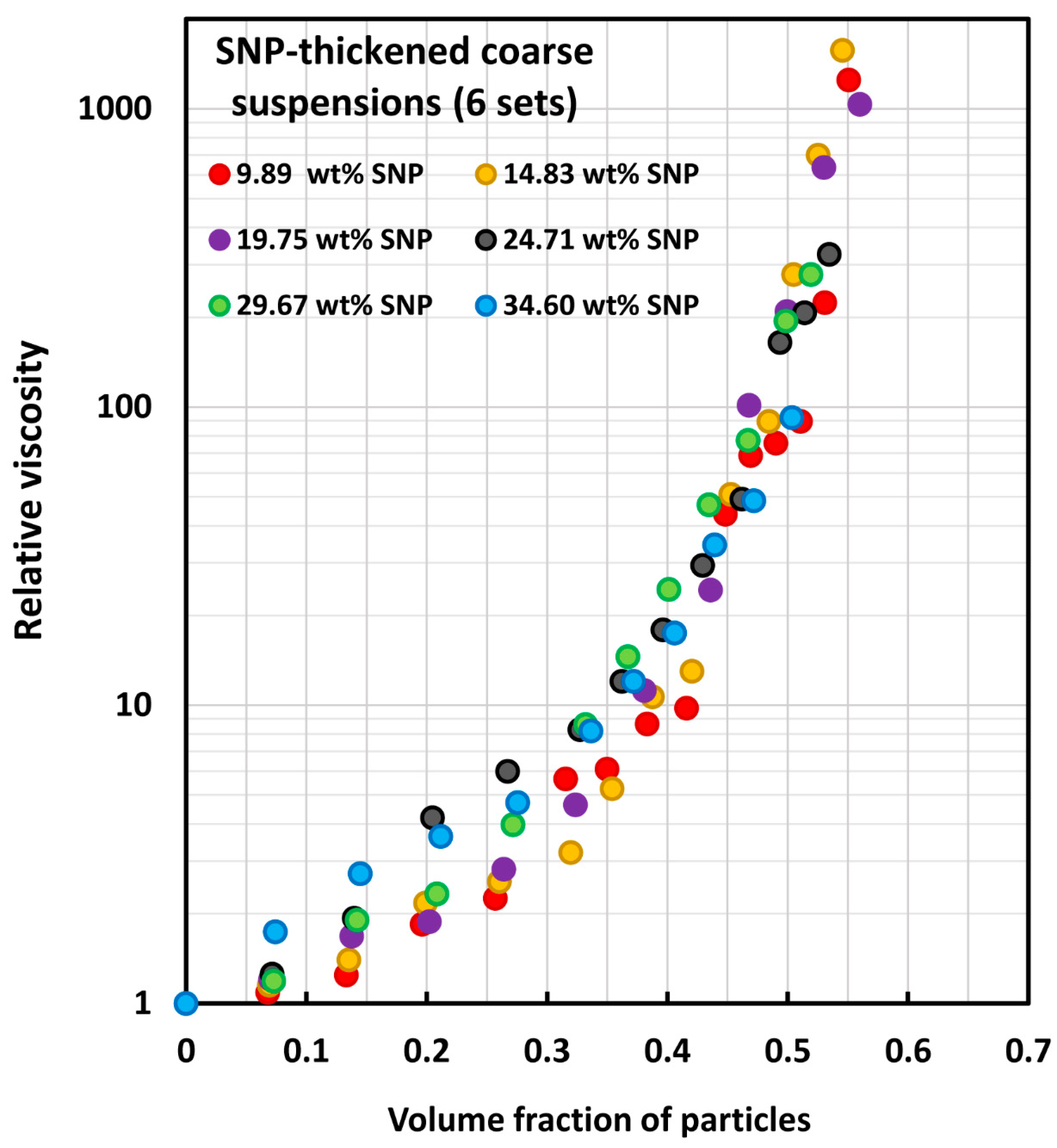
| Set No | SNP Concentration of Matrix Phase (wt%) | Type and Size of Solid Particles | Concentration Range of Solid Particles (vol%) | Reference |
|---|---|---|---|---|
| 1–6 | Set 1 (9.89%), set 2 (14.83%), set 3 (19.75%), set 4 (24.71%), set 5 (29.67%), set 6 (34.60%) | Ceramic hollow spheres, 10 to 340 µm; Sauter mean diameter of 138 µm | Set 1 (0–55.08%), set 2 (0–54.54%), set 3 (0–56%), set 4 (0–53.44%), set 5 (0–51.93%), set 6 (0–50.36%) | Ghanaatpishehsanaei and Pal [82] |
| Model Type | Coarse Suspensions | Nanosuspensions | SNP-Thickened Coarse Suspensions |
|---|---|---|---|
| Mooney model (M) | −8.98 × 10⁸% (Overpredicts extremely) | −1.64 × 10¹⁸% (Overpredicts extremely) | −3.88 × 1031% (Overpredicts extremely) |
| Krieger–Dougherty model (KD) | 27.55% (Underpredicts substantially) | 23.05% (Underpredicts substantially) | 47.73% (Underpredicts severely) |
| Cheng et al. model (C) | −3531% (Overpredicts extremely) | −1.14 × 10⁷% (Overpredicts extremely) | −2.16 × 10²²% (Overpredicts extremely) |
| Mendoza and Santamaria-Holek model (MS) | 12.56% (Underpredicts substantially) | 10.43% (Underpredicts substantially) | 23.96% (Underpredicts substantially) |
| Brouwers model (B) | −21.6% (Overpredicts substantially) | −32.43% (Overpredicts severely) | −43.4% (Overpredicts severely) |
| Pal model one (P1) | −34.81% (Overpredicts severely) | −26.01% (Overpredicts severely) | −56.42% (Overpredicts severely) |
| Pal model two (P2) | 24.85% (Underpredicts substantially) | 22.96% (Underpredicts substantially) | 42.64% (Underpredicts severely) |
| Pal model three (P3) | 3.22% (Underpredicts slightly) | 3.51% (Underpredicts slightly) | 6.37% (Underpredicts moderately) |
| 0.50 | 0.21 | 8.18 | 0.41 | 0.33 | 0.26 |
| 0.55 | 0.23 | 12.07 | 0.42 | 0.33 | 0.25 |
| 0.60 | 0.26 | 19.10 | 0.44 | 0.32 | 0.24 |
| 0.65 | 0.30 | 33.26 | 0.45 | 0.32 | 0.23 |
| 0.70 | 0.33 | 66.28 | 0.47 | 0.32 | 0.21 |
| 0.75 | 0.37 | 161.98 | 0.49 | 0.31 | 0.20 |
| 0.80 | 0.42 | 555.34 | 0.52 | 0.30 | 0.18 |
| 0.85 | 0.47 | 3662.97 | 0.55 | 0.29 | 0.16 |
| 0.89 | 0.52 | 49,779.29 | 0.59 | 0.28 | 0.13 |
Disclaimer/Publisher’s Note: The statements, opinions and data contained in all publications are solely those of the individual author(s) and contributor(s) and not of MDPI and/or the editor(s). MDPI and/or the editor(s) disclaim responsibility for any injury to people or property resulting from any ideas, methods, instructions or products referred to in the content. |
© 2023 by the author. Licensee MDPI, Basel, Switzerland. This article is an open access article distributed under the terms and conditions of the Creative Commons Attribution (CC BY) license (https://creativecommons.org/licenses/by/4.0/).
Share and Cite
Pal, R. Recent Progress in the Viscosity Modeling of Concentrated Suspensions of Unimodal Hard Spheres. ChemEngineering 2023, 7, 70. https://doi.org/10.3390/chemengineering7040070
Pal R. Recent Progress in the Viscosity Modeling of Concentrated Suspensions of Unimodal Hard Spheres. ChemEngineering. 2023; 7(4):70. https://doi.org/10.3390/chemengineering7040070
Chicago/Turabian StylePal, Rajinder. 2023. "Recent Progress in the Viscosity Modeling of Concentrated Suspensions of Unimodal Hard Spheres" ChemEngineering 7, no. 4: 70. https://doi.org/10.3390/chemengineering7040070