
The Rating Scale Paradox: Semantics Instability versus Information Loss


1
SACE S.p.A, Piazza Poli 42, 00187 Rome, Italy
2
Department of Statistics, Sapienza University of Rome, Viale Regina Elena 295, 00161 Rome, Italy
†
The views and opinions expressed in this article are those of the author and do not necessarily reflect the official policy or position of SACE S.p.A.
Standards 2022, 2(3), 352-365; https://doi.org/10.3390/standards2030024
Submission received: 26 June 2022
/
Revised: 20 July 2022
/
Accepted: 25 July 2022
/
Published: 1 August 2022
(This article belongs to the Special Issue Exclusive Papers Collection of Editorial Board Members and Invited Scholars in Standards)
Abstract
:Rating systems are applied to a wide variety of different contexts as a tool to map a large amount of information to a symbol, or notch, chosen from a finite, ordered set. Such a set is commonly known as the rating scale, and its elements represent all the different degrees of quality—in some sense—that a given rating system aims to express. This work investigates a simple yet nontrivial paradox in constructing that scale. When the considered quality parameter is continuous, a bijection must exist between a specific partition of its domain and the rating scale. The number of notches and their meanings are commonly defined a priori based on the convenience of the rating system users. However, regarding the partition, the number of subsets and their amplitudes should be chosen a posteriori to minimize the unavoidable information loss due to discretization. Considering the typical case of a creditworthiness rating system based on a logistic regression model, we discuss to what extent this contrast may impact a realistic framework and how a proper rating scale definition may handle it. Indeed, we show that choosing between a priori methods, which privilege the meaning of the rating scale, and a posteriori methods, which minimize information loss, is not strictly necessary. It is possible to mix the two approaches instead, choosing a hybrid criterion tunable according to the rating model’s user needs.
1. Introduction
Nowadays, the application of rating systems is widespread in a remarkable variety of contexts. Indeed, almost any real-life decisional process requires the ability to order a set of items (objects or subjects) based on a quality criterion. From the triage color coding used to classify the severity of each case in hospitals [1,2,3] to the ELO system [4], and its further evolutions [5,6], used to compare players in chess and other competitive zero-sum games, the examples are most diverse.
As stated above, a rating system is a means to sort a set and uniquely associate a “state”, or notch, to each element. Such a function is mainly intended for two purposes. First, it offers a quick summary of the data used to perform the classification: e.g., the rating issued by a credit rating agency provides the investors with information far more easily understood than the collection of financial statements available from the rated firm. Second, it enables decisional processes and their possible automation. This paper investigates the possible conflict between these two apparently coherent purposes. In this work, we highlight the existence of a problem that is nearly as common as the rating systems applications themselves but not as acknowledged.
In order to be effective, a rating system needs to keep all the complexity “hidden” in the classification process and provide the final user with simple, standardized output. The simplicity is commonly achieved by defining the codomain of the rating system’s function as a finite or, at least, discrete, set of states—the so-called “master scale”, or “rating scale” [7,8,9].
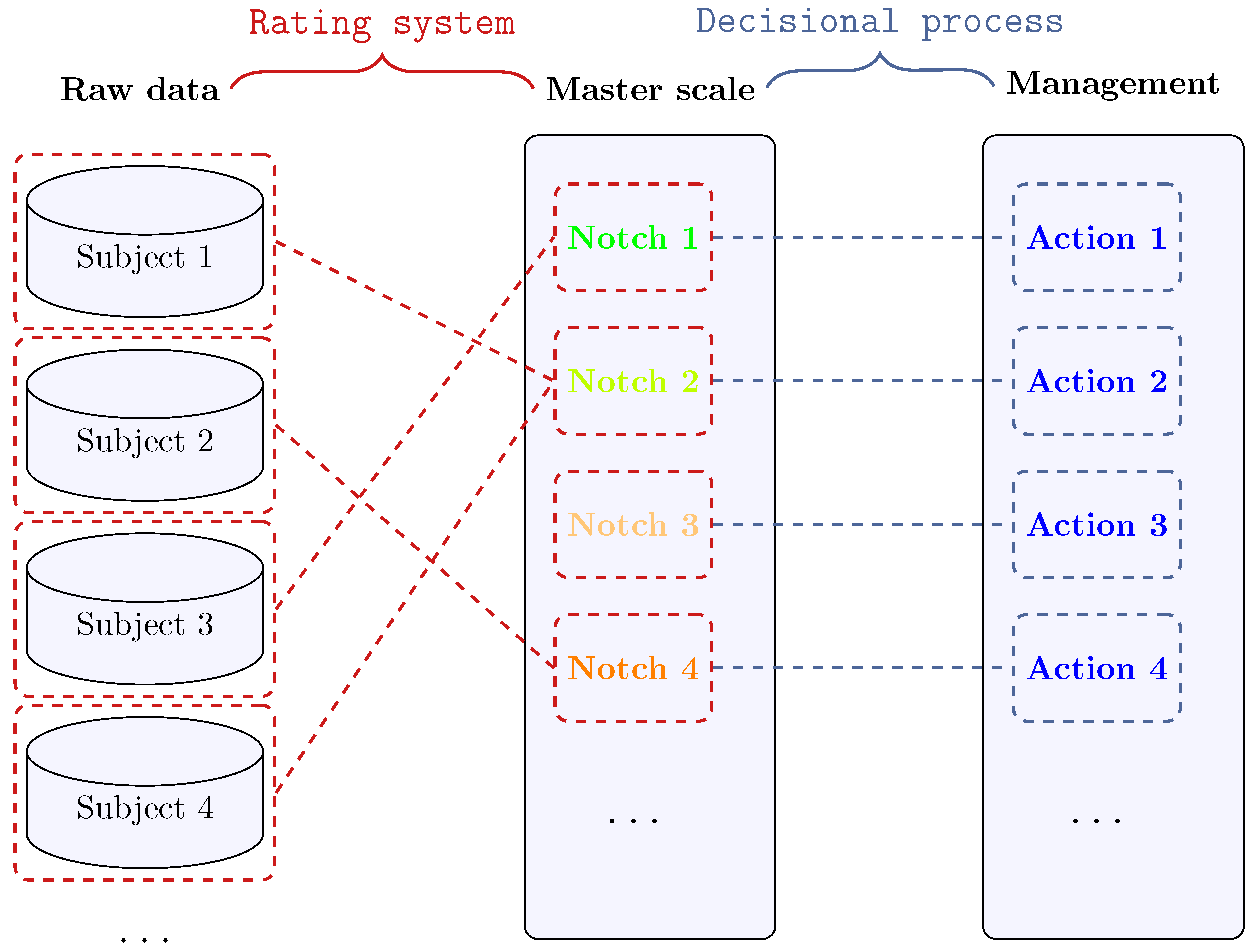
The master scale is often a reference to implement strategies and make decisions. To highlight this fact, let us consider the abovementioned examples. A bank may reject a loan request or grant it up to a given exposure based on the client’s credit score. Nurses follow different protocols based on the triage color assigned to the patient. Professional chess players earn different titles based on the ELO score they can reach and maintain, together with the right to join specific tournaments. These examples share a common feature: each notch of the master scale is uniquely associated with a specific set of actions and rules, implying that the decisional system can be represented as a bijective map.
The “rigid” decisional map depicted in Figure 1 is well-posed only if the master scale’s semantics is as rigid. Namely, if a given notch always implies the same actions over time, the meaning of the notch must be stable over time as well. As stated above, the rating system is de factoa means to order a given population and partition it into subsets. The master scale corresponds to the partition applied after sorting the population. Hence, the master scale can be kept stable through time without losing information or altering its semantics only if the population distribution is stationary. Unfortunately, this is not the case in many contexts.
The seminal background needed to design a master scale dates back to the early twentieth century, when American rating agencies began developing the tools needed for their activity [10]. In the meanwhile, flourishing research activity in psychology [11,12], being still ongoing nowadays [13,14], was devoted to designing master scales as a tool to map subjective attitudes collected through questionnaires into a quantitative framework. It is worth noticing that the schema reported in Figure 1 also holds in the latter context, considering the subjective attitudes as raw data and the questionnaire’s structure as the rating system.
The problem mentioned above of a master scale’s stability over time is just partly addressed in credit risk literature [15]. The proposed solutions are focused on improving the precision of the estimated probability of default associated with each notch as possible (see, e.g., [16]) and validating the (previously calibrated) master scale [17,18]. In Falkenstein’s approach to master scale validation [17], the estimation of default and recovery rates per notch plays a central role, while Sobehart [18] proposed to also apply information criteria (e.g., accuracy ratio, information entropy) to assess the overall performance of the rating system. However, the banking and finance literature does not offer a precise, unique solution to the problem of calibrating a master scale’s partition in the presence of a non-stationary population. Indeed, in corporate default risk applications, the problem is mitigated by the stability obtained through calibrating default probabilities over an extended observation period [7,8].
Coming back to the ELO example and its stability, there is an ongoing debate about the so-called “rating inflation”. In fact, there is a possible distortion of the ELO semantics due to the evolution of the chess players’ population, implying that a contemporary player with a given ELO score is probably weaker than a player rated with the same ELO score decades ago. If this is confirmed, the decision system or the rating system should be adjusted to avoid that being awarded a given title (e.g., “international master”) requires lesser skills over time, given the same ELO score threshold. The question is open to date, and some analyses suggest that such a phenomenon is hardly detectable [19]. Nonetheless, FIDE addresses it by fine-tuning its rating system parameters over time [20].
The triage systems’ stability has been recently impacted worldwide as well. Indeed, in this context, the COVID-19 pandemic shows that the severity distribution of human illness in any country is subjected to abrupt changes that require reviewing the triage master scale semantics and its implications on the related decisional process [21,22].
In the following, we consider another ubiquitous rating system: credit scoring based on logistic regression. In this work, we discuss how the semantics stability of the master scale and the preservation of information can conflict even in such a simple and widely applied system, forcing the user to update the notchs’ meaning by time (and the related decisional system as well) or to lose information as the evaluated population evolves. It is worth recalling a typical strategy that the banking industry and rating agencies adopt to address this problem, that is, the through-the-cycle calibration of the probabilities of default (also “PD”) considered by the rating model. This choice guarantees the master scale’s stability for practical purposes, provided that the subsequent decisional process is long-term oriented. However, financial intermediaries also need to evaluate PDs and subsequent decisions in a short-term framework (see, e.g., [23,24]), implying the inapplicability of a through-the-cycle approach to fix the problem.
The remainder of the paper is organized as follows. Section 2 describes a typical rating system based on logistic regression, together with some possible methods to define the rating scale. Section 3 compares the outcomes of the different methods given the same population and underlying scoring model. Section 4 extends the comparison by introducing a toy decisional system and showing the impact of considering a method that privileges semantics stability or a method oriented to minimize information loss. The benefits of a hybrid method are discussed as well. Section 5 summarizes the main results obtained in this work.
2. Models and Methods
This section recalls the theoretical framework used in this work. Section 2.1 describes some of the main features of a rating model based on a logistic regression model. Without claim to completeness, Section 2.2 proposes a selection of different methods to evaluate the master scale, considering both the “fixed semantics” and the “maximum information” criteria.
2.1. A Typical Rating System
A credit scoring model can be thought of as a map from a set of measured attributes of the evaluated subject—typically microeconomic variables—to a PD value or, at least, a symbolic notch that expresses a certain creditworthiness level.
In this perspective, such a model can be classified into the wider category of “structural” models, whose the first and most remarkable example is the Merton–KMV model [25,26,27]. Typically, a structural model is based on two assumptions:
- i.
- The deterministic relationship existing between a set of microeconomic variables describing the state of a firm and its creditworthiness;
- ii.
- The stochastic marginal dynamics of the considered microeconomic variables.
However, this setting is not shared among all the structural models. A comprehensive class of structural models—known as “cross-sectional” models—represents a commonly accepted approach to model the default probability PD of a firm as a function of the information available from the firm’s financial statements without introducing any additional assumptions about dynamics [28]. This class coincides with credit scoring models.
In a nutshell, a typical credit scoring model is based on the hypothesis that the PD of a firm F, estimated in t over a given time horizon , can be expressed as a generalized linear function of some financial ratios and/or other numerical values taken from the firm’s financial statements.
where is the time to default of F, is the array of the model parameters to be calibrated and is the value of the i-th considered variable, measured in t from the F’s financial statements and/or other selected information sources.
The function is chosen according to tractability criteria. Unlike in Merton model, in this case, there are no assumptions about the dynamics of creditworthiness that imply a form of . A comparative analysis on the presence of each cross-sectional model in the literature can be found in [29]: the “logit” and “probit” models emerge as the most commonly studied in terms of number of papers. These two typical choices [28,29,30] correspond to taking as the standard logistic function
and the standard normal CDF
where is the error function.
In this context, it is commonly assumed that default events over are distributed as i.i.d. Bernoulli random variables conditionally to the state of each firm. Under this assumption, the two forms listed above lead to the “logit” and “probit” models, respectively. A reason for the popularity of these models is the possibility to calibrate them by maximum likelihood (ML) estimation of their parameters from historical data. Indeed, the likelihood function can easily be written in closed form due to the independence among defaults.
where , and .
Furthermore, in both cases, the optimal parameter choice is easily achievable due to the computable form of the first derivative: in the logit model, can be represented as a closed-form expression of , since the logistic function is a solution to the differential equation , while in the probit model, is the standard normal PDF. Generally speaking, the choice between the two models is not relevant to practical purposes in most cases since their outcomes are very similar [30,31].
In banking practice, this technique is commonly embedded in a wider framework [9,31,32] (i.e., an internal rating system), applied to assess the credit risk profile of risky debtors who belong to the same homogenous cluster.
In this context, a cluster of debtors is “homogenous” if their PDs are supposed to be related to the same predictors’ array by the same parameter set . Typical examples of homogeneous clusters consist of enterprises that belong to the same segment, economic sector, and geographical area (e.g. European financial large corporate; US agricultural small/medium enterprises).
Without a claim to completeness, some of the elements that are usually introduced to apply a “logit”/“probit” model (or other comparable approaches) to practical purposes are listed below:
- a.
- Univariate selection of the variables to be included among predictors , according to a measure of their diagnostic ability;
- b.
- Multivariate validation of the selected predictors and dimensionality reduction of by the application of PCA or another factor analysis technique;
- c.
- Partition of the PD domain in a finite set of indexed subintervals (i.e., rating classes, also known as grades), each of them being associated with a symbol (e.g. AA, A, BBB, etc.) and with a qualitative description of the corresponding risk level (the so-called “master scale”);
- d.
- Allowance for expert-judgment-based override of the rating, leading to a joint usage of quantitative and qualitative results to produce a final evaluation of the firm creditworthiness.
Elements “a” and “b” concern the definition of the scoring model, while element “d” is well-posed only after having calibrated the master scale. On the other hand, element “c”, the introduction of a master scale extending the scoring model in a rating system, is the central topic of this work.
It is relevant to note that the complete specification of a rating model still needs the estimation of historical default rates and forward-looking default probabilities in the same portfolio/cluster to which the model is being applied [9,32,33,34].
ML calibration on historical data is based on -long observations (with typically equal to 1 year) of defaulted/survived enterprises collected in a past period that spans several years (i.e., a whole economic cycle or more). The resulting default rate associated with the calibration sample is a long-run average, and the “natural” map grade↔PD is built accordingly.
However, a financial entity may be interested in defining a different master scale. From a short-term perspective, the forward-looking PDs expected for the next year could be significantly far from the long-run average (either above or below). Depending on the considered application, the short-term level, known as point-in-time (PIT) PD, often results in being more appropriate, and thus, the master scale has to be adjusted to reflect an average PIT PD level across the grades instead of the natural long-term PD level.
Indeed, according to “The Internal Ratings-Based Approach” (BIS, 2001) [32], Section E, paragraph 54, p. 12, banks tend to consider the PIT PD level more often than the long-run average PD. Moreover, IFRS 9 standard (see [35], paragraph B5.5.52) requires the estimation of a PIT PD, as discussed in [34].
In the literature, the PIT PD concept is usually contrasted with the through-the-cycle (TTC) PD. It is worth noticing that “TTC” is a slightly ambiguous expression. Indeed, some authors identify the TTC PD with the long-run average PD level through a whole economic cycle, as its name suggests (see, e.g., [34]). However, according to the Basel Committee, the concept of TTC PD is associated with a prudential long term PD level, instead of the average default rate observed. Considering this second possible meaning, the application of the TTC PD level to the master scale also requires an adjustment.
Indeed, “The Internal Ratings-Based Approach” (BIS, 2001) [32], Section E, paragraph 53, p. 12, reads: “[…] In a point-in-time process, an internal rating reflects an assessment of the borrower’s current condition and/or most likely future condition throughout the chosen time horizon. As such, the internal rating changes as the borrower’s condition changes throughout the credit/business cycle. In contrast, a through-the-cycle process requires assessment of the borrower’s riskiness based on a worst-case, bottom-of-the-cycle scenario (i.e., its condition under stress). In this case, a borrower’s rating would tend to stay the same throughout the credit/business cycle.”.
Several techniques are available in the literature to adjust the PD associated with each grade in a master scale. The seminal work of Falkenstein et al. [31] suggests to scale each PD in the master scale by the coefficient such that the average PD in the calibration sample is equal to the target PD level (i.e., PIT/TTC/other). Hence, this approach implies that the shape of the PD profile, as a function of the grade, must not be affected by the adjustment. A discussion where this choice is compared with other non-uniform adjustment techniques is available in [33].
2.2. Considered Partition Criteria
Let the function be the master scale of our rating model:
where the score s is defined as
The score threshold array
fully specifies the master scale. In the following, five distinct criteria are introduced to evaluate . Section 2.2.1 presents a straightforward way to fix the meaning of each notch, detaching the master scale semantics from the underlying population and its evolution. Section 2.2.2, Section 2.2.3 and Section 2.2.4 propose three non-equivalent criteria to minimize the information loss occurring when the master scale is applied. The four methods are used and compared in Section 3. Finally, Section 2.2.5 proposes to combine the semantics-based and the information-based criteria. The possible benefits of this choice are discussed in Section 4.
2.2.1. Fixed Semantics
A possible purpose of a rating model is to serve as the basis of a rigid decisional system. Each notch must maintain the same meaning over time to guarantee that the initially associated action is appropriate. In the credit risk context, the meaning of each notch is determined by the PD distribution of the corresponding sub-population. Hence, setting constant threshold levels of PD between subsequent notches is a possible and plain criterion to fix the semantics. Namely, the score partition is directly implied by the chosen PD thresholds:
where . For example, another possible criterion is to fix the expected PD value associated with each notch r (except for the worst and/the best notch to avoid an overdetermined set of constraints). However, the two methods have no relevant differences with respect to our purposes. In the remainder of this work, is the only fixed semantics criterion considered, although the same results can be obtained with other similar criteria.
2.2.2. Maximum Hit Rate
The hit rate [36,37] is commonly measured when assessing the predictive power of a rating system. Let us consider a sample population of M individuals where D default events have already been observed over a given period. is defined as the area under the curve
When evaluating a master scale, in Equation (9) becomes
where is the number of r-rated individuals, and is the number of defaulted r-rated individuals. Thus, the hit ratio is measured as a sum of trapezoid areas:
It is worth noticing that can be thought of as a function of , which is needed to compute , ().
Increasing values of correspond to a greater predictive power of the model, as a stronger separation between the distributions of defaulted and not defaulted individuals is implied by construction. Hence, the master scale
minimizes the loss of predictive power when turning the scoring model in a rating model.
2.2.3. Maximum Likelihood
The same functional form considered in Equation (4) to calibrate can be applied to also calibrate
where is the average PD among the sub-population of r-rated debtors. The partition
minimizes the likelihood reduction when turning the scoring model in a rating model.
2.2.4. Minimum Kullback–Leibler Divergence
The last information criterion that we propose and discuss in the numerical comparison reported in Section 3 is the Kullback–Leibler divergence () [38], also known as relative entropy. In a nutshell, measures the loss of information undergone when using a distribution Q to describe a phenomenon whose true distribution is P. In our framework, P is the probability distribution implied by the scoring model, while Q is the probability distribution implied by scoring model conversion to a discrete rating model. Namely, we have
Additionally, depends on , which is needed to compute . Hence, may be chosen to minimize the information loss:
2.2.5. Hybrid Criteria
It is easily verified that, given two (increasingly) ordered sets and , any elementwise weighted average
preserves the ascending order. This trivial property allows us to combine master scales obtained by the application of different criteria, obtaining another well-defined master scale. In particular, it is possible to mix a master scale based on a semantics criterion and one based on an information criterion, aiming to obtain the advantages of both to some extent. In Section 4, we propose the hybrid criterion
3. Numerical Comparison among Different Partition Criteria
This section compares the methods introduced in Section 2.2.1, Section 2.2.2, Section 2.2.3 and Section 2.2.4 through their application to a specific set of scenarios defined in a simplified framework. The numerical setup is described in the next Section 3.1. Comments on the results obtained from the application of the fixed semantics and the maximum information criteria are available in Section 3.2 and Section 3.3, respectively.
3.1. Numerical Setup
Let us consider a population of risky debtors whose 1-year PDs obey the law
over the interval . Let us consider a perfectly calibrated logistic scoring model, where it holds that . In this way, we are able to isolate and study the effects of our choices concerning , avoiding them to be affected by the error made in estimating . Further, we assume that . The sign of the weights implies no loss of generality, given that a minus sign can be absorbed in a re-definition of the corresponding variable. As already stated in Section 1, we expect partitions defined out of an information criterion to show a strong degree of flexibility in the presence of a relevant portfolio evolution. To simulate increasingly worsening scenarios, we assume that all the variables have normal distribution across the debtors, and both their mean and standard deviation increased linearly through the scenarios. In particular, we have and , with , resulting in the PD distribution per scenario depicted in Figure 2. All the results reported in this section and the next one have been obtained by implementing in R language the specifications described in this work.
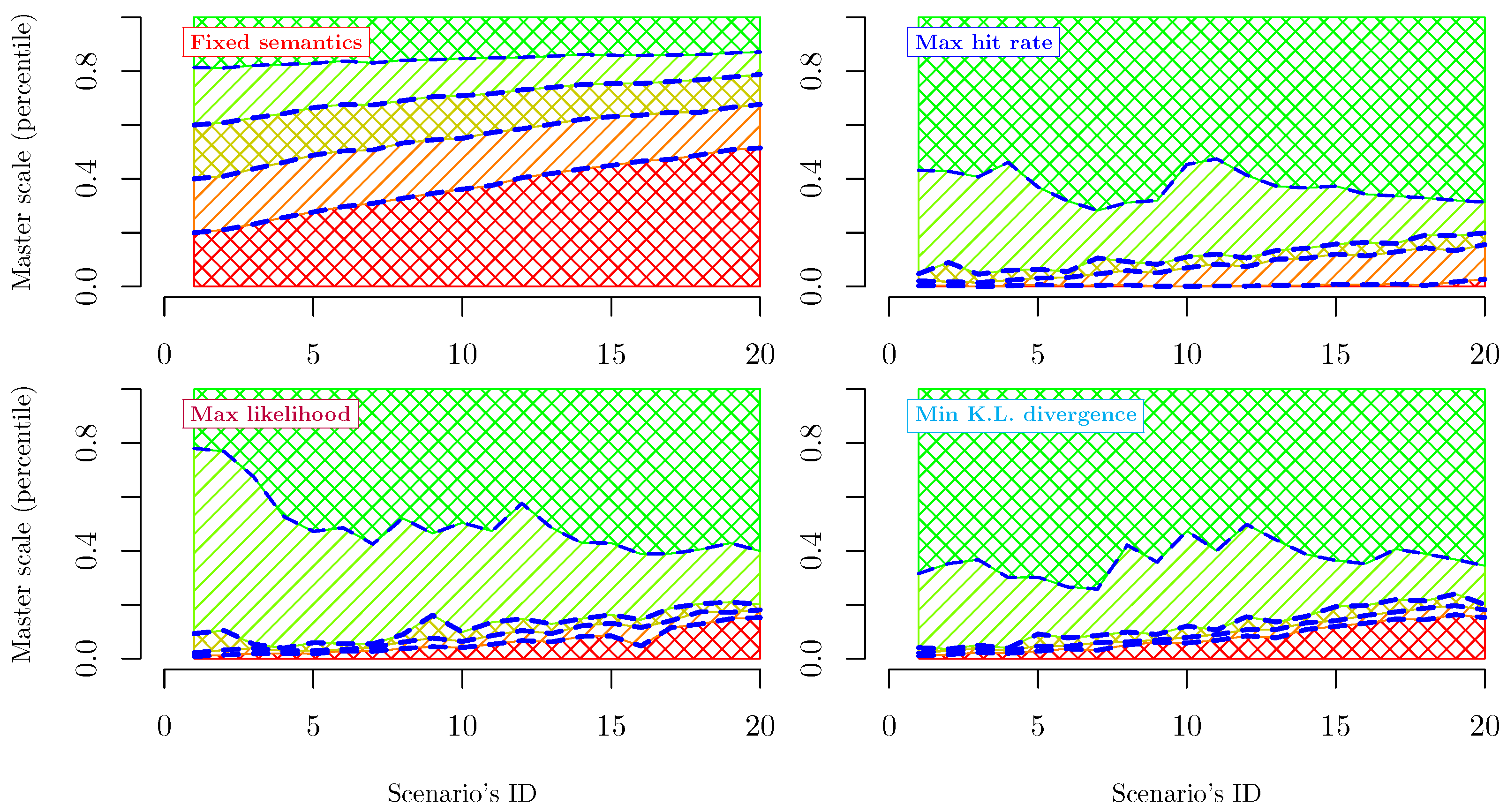
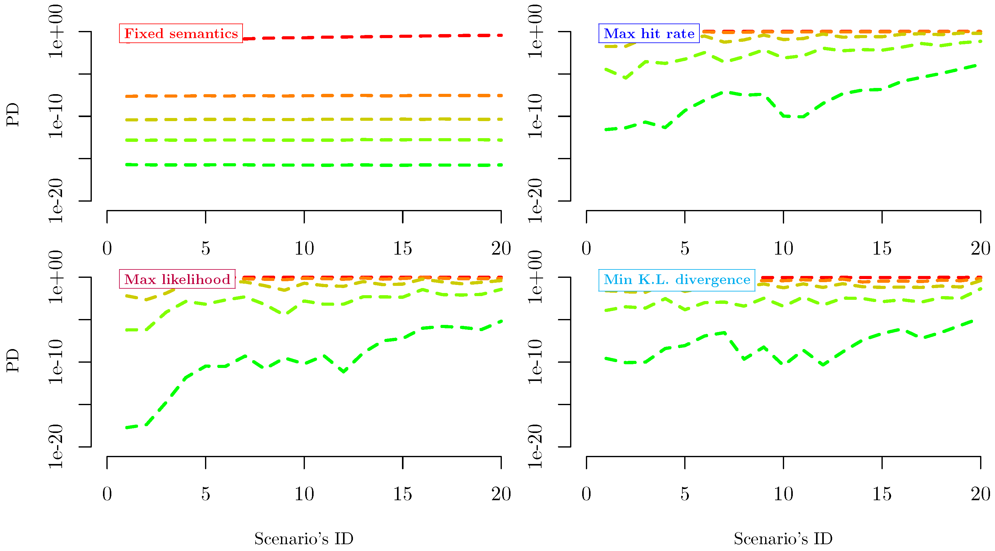
Criteria introduced in Section 2.2.1, Section 2.2.2, Section 2.2.3 and Section 2.2.4 are applied through all the aforementioned scenarios to calibrate a 5-notch rating system. Figure 3 and Figure 4 compare the results obtained per method/scenario. Information critera, despite not being equivalent, lead to very similar outcomes, while the only semantics-based criterion considered exhibits a remarkably distinguished behavior. Further considerations are reported in the following Section 3.2 and Section 3.3.
3.2. Features of Fixed Semantics Criteria
The considered fixed semantics method lets the PD evolution directly affect the number of subjects per notch. Indeed, increasing PDs across the considered scenarios leads to more populated low-creditworthiness notches (Figure 3, top left panel). Conversely, the notches associated with high-standing debtors get progressively emptier as the PDs grow.
Across the whole PDs’ evolution, the average PD per notch remains almost stable (Figure 4, top left panel), as each threshold PD between two subsequent notches is fixed. The latter would have been precisely true if we selected the average PD per notch as a semantics-based criterion. Obtaining approximately the same results by choosing a fixed threshold criterion highlights that different semantics-based criteria produce comparable results.
As further discussed in Section 4, such a rating scale, if coupled with a rigid decisional system (e.g., refuse any exposure on 5-rated debtors), copes with the needs of a rating model’s user (e.g., a commercial bank) who is risk-averse and aims at long-term profit. Indeed, such an entity accepts a low business volume during adverse macroeconomic phases (i.e., high PDs) to minimize the losses, increasing the business volume only in periods when the average PD is lowering.
3.3. Features of Maximum Information Criteria
Unlike semantics-based criteria, all the considered information-based criteria show pronounced PD-per-notch dynamics (Figure 4) and the tendency to keep the worst notch population as low as possible (Figure 3). These effects are accentuated by the perfect calibration that we assumed in Section 3.1.
The specific ability of the scoring model to identify the highest-PD subjects makes it more efficient to isolate them in a small-populated notch and leave the remaining four notches to differentiate more precisely the remainder of the population. Further, the almost-zero amplitude of the central notch suggests that four notches instead of five would provide a more efficient description of the evaluated population.
As further discussed in Section 4, such a dynamic rating scale fits the needs of a rating model’s user (e.g., a venture capital firm) whose strategy encompasses invested volumes to be as high as possible, and diversified among several accepted risks. Thus, such an entity wants to reject only the riskiest debtors, which must be identified as precisely as possible.
4. Relative Evaluations and Absolute Decisions: Rating System Applied in a RAF
Semantics-based and information-based calibrations of the master scale lead to remarkably different outcomes, as highlighted by the simulations shown in Section 3. The results presented so far do not suggest that one of the two approaches is to be preferred over the other. Both seem appropriate, depending on the risk vs. volume appetite of the model’s user. Hence, the hybrid criterion proposed in Section 2.2.5 is a natural candidate to fit for intermediate situations, where neither pure semantics-based criteria nor information-based criteria perfectly satisfy the model’s user needs. This section aims to complete the analysis presented in Section 3 focusing on this aspect.
Considering the schema reported in Figure 1, we need to complete our simplified framework with a decisional process associated with the rating system to assess the practical effects of the two approaches. Let us assume that the rating system calibrated in Section 3 is applied by a generic financial entity (e.g., bank, factor, or credit insurance) that has implemented an automated strategy to grant exposure depending on the rating outcome. In particular, the exposure granted to the j-th subject is defined as an exponential function of the rating
so that the worst rating (i.e., ) implies a rejection of all the exposure’s requests, while the best rating grants the maximum exposure , where the currency units are arbitrary and not relevant.
Just by adding Equation (21) to the picture, we now have a complete—although “toy”—risk appetite framework (RAF) [24], where the financial consequences of the two approaches are observable.
As shown in Figure 5 and Figure 6, the semantics-based approach is the most prudential from a risk appetite perspective. This result copes with intuition. Indeed, as the population’s creditworthiness decreases across the scenarios, the master scale thresholds are not reviewed. Thus, an increasing number of subjects become 5-rated and not eligible for positive exposure.
On the other hand, the information-based approaches lead to a stable exposure, which is more than three times the one implied by the semantics-based master scale, as the subjects which were 3-to-5-rated are located only in the right tail of the PD distribution.
Not surprisingly, the relative expected loss is higher when applying one of the information-based criteria, as shown in Figure 6. However, it is remarkably stable across the scenarios for each considered criterion. Hence, no method has flaws that imply its a priori exclusion for practical purposes. The right choice depends on the size of the financial entity applying the RAF, its own risk appetite level, and the market context. An increasing volume of exposure (i.e., a greater market share) is preferable, conditioned to fair pricing and available own funds, which must be large enough to retain the credit risk.
Thus, the right choice for a specific entity can be identified by the entity itself through an interpolation between the optimal semantics-based and information-based master scales, as proposed in Section 2.2.5. In Figure 7, we have numerically verified that the smooth transition from () to () generates smooth and per scenario, allowing each entity to identify its optimal decisional framework according to its specific risk appetite.
5. Conclusions
We have outlined two different approaches to defining a generic rating scale. The first is a priori (semantics-based). It does not take into account the features of the evaluated population, implying a constant meaning of each notch and guaranteeing that a given creditworthiness level always implies the same action, regardless of the context. The second is a posteriori (information-based) and aims to process and preserve the available information most efficiently. However, doing so implies that an automated decisional framework is adapted to the evolving context, and the same creditworthiness level may imply different decisions in different market scenarios.
The presented results are obtained by considering a credit risk application of rating systems. However, their implications are easily extended to any other context: a standard method to define a rating scale is missing to date because looking for it is an ill-posed problem.
Indeed, the best rating scale is the one that has the most desirable impact on the entity that uses it as the basis of a subsequent decisional process. What “desirable” means depends on the entity’s features and the market context, as highlighted by the toy model numerically investigated in Section 3 and Section 4. Thus, the main original contributions in this work are the distinction between semantics-based and information-based techniques and the proposed solution to mix them according to the needs of the model’s user.
This study is limited to introducing two categories to classify the rating scale calibration methods and proposing a new class of hybrid criteria. Practical applications to real-life cases require considering all the business and regulatory features of a given entity (e.g., bank, insurance company, investment fund, corporate firm), possibly leading to remarkably different results. This level of realism in technical specifications is beyond this work’s aim and scope and deserves to be further considered case-by-case in future research works.
Funding
This research received no external funding.
Data Availability Statement
Not applicable.
Conflicts of Interest
The author declare no conflict of interest.
References
- Hodgetts, T.J.; Hall, J.; Maconochie, I.; Smart, C. Paediatric triage tape. Prehosp. Immed. Care 2013, 2, 155–159. [Google Scholar]
- Cross, K.P.; Cicero, M.X. Head-to-head comparison of disaster triage methods in pediatric, adult, and geriatric patients. Ann. Emerg. Med. 2013, 61, 668–676. [Google Scholar]
- Lerner, E.B.; McKee, C.H.; Cady, C.E.; Cone, D.C.; Colella, M.R.; Cooper, A.; Coule, P.L.; Lairet, J.R.; Liu, J.M.; Pirrallo, R.G.; et al. A consensus-based gold standard for the evaluation of mass casualty triage systems. Prehosp. Emerg. Care 2015, 19, 267–271. [Google Scholar]
- Elo, A.E. The Proposed USCF Rating System. Chess Life 1967, XXII, 242–247. Available online: http://uscf1-nyc1.aodhosting.com/CL-AND-CR-ALL/CL-ALL/1967/1967_08.pdf (accessed on 21 June 2022).
- Glickman, M.E. Parameter estimation in large dynamic paired comparison experiments. Appl. Stat. 1999, 48, 377–394. [Google Scholar]
- Veček, N.; Mernik, M.; Črepinšek, M.; Hrnčič, D. A Comparison between Different Chess Rating Systems for Ranking Evolutionary Algorithms. In Proceedings of the 2014 Federated Conference on Computer Science and Information Systems, Warsaw, Poland, 7–10 September 2014; Ganzha, M., Maciaszek, L., Paprzycki, M., Eds.; 2014; Volume 2, pp. 511–518. [Google Scholar]
- Rating Symbols and Definitions. Moody’s Investors Service. 2 June 2022. Available online: https://www.moodys.com/researchdocumentcontentpage.aspx?docid=pbc_79004 (accessed on 21 June 2022).
- Oosterveld, B.; Bauer, S. Rating Definitions. FitchRatings Special Report, 21 March 2022. Available online: https://www.fitchratings.com/research/structured-finance/rating-definitions-21-03-2022 (accessed on 21 June 2021).
- Nehrebecka, N. Probability-of-default curve calibration and validation of internal rating systems. In Proceedings of the 8th IFC Conference on “Statistical Implications of the New Financial Landscape”, Basel, Switzerland, 8–9 September 2016; Available online: https://www.bis.org/ifc/publ/ifcb43_zd.pdf (accessed on 21 June 2021).
- Weissova, I.; Kollarb, B.; Siekelova, A. Rating as a Useful Tool for Credit Risk Measurement. Procedia Econ. Financ. 2015, 26, 278–285. [Google Scholar]
- Thurstone, L.L. Theory of attitude measurement. Psychol. Rev. 1929, 36, 222. [Google Scholar]
- Likert, R. A technique for the measurement of attitudes. Arch. Psychol. 1932, 22, 55. [Google Scholar]
- Parducci, A. Category ratings and the relational character of judgment. Adv. Psychol. 1983, 11, 262–282. [Google Scholar]
- Menold, N.; Wolf, C.; Bogner, K. Design aspects of rating scales in questionnaires. Math. Popul. Stud. 2018, 25, 63–65. [Google Scholar]
- Carey, M.; Hrycay, M. Parameterizing credit risk models with rating data. J. Bank. Financ. 2001, 25, 197–270. [Google Scholar]
- Delianis, G.; Geske, R. Credit Risk and Risk Neutral Default Probabilities: Information about Rating Migrations and Defaults. Working Paper, UCLA. Available online: https://escholarship.org/uc/item/7dm2d31p (accessed on 20 July 2022).
- Falkenstein, E. Validating commercial risk grade mapping: Why and how. J. Lend. Credit. Risk Manag. 2000, 82, 26–33. [Google Scholar]
- Sobehart, J.R.; Keenan, S.C.; Stein, R.M. Benchmarking Quantitative Default Risk Models: A Validation Methodology; Moody’s Investors Service: New York, NY, USA, 2020; Available online: http://www.rogermstein.com/wp-content/uploads/53621.pdf (accessed on 20 July 2022).
- Regan, K.W.; Macieja, B.; Haworth, G.M. Understanding distributions of chess performances. In Advances in Computer Games; Springer: Berlin/Heidelberg, Germany, 2011; pp. 230–243. [Google Scholar]
- FIDE Rating Regulations Effective from 1 January 2022. Available online: https://www.fide.com/docs/regulations/FIDE%20Rating%20Regulations%202022.pdf (accessed on 21 June 2022).
- Brindle, M.E.; Doherty, G.; Lillemoe, K.; Gawande, A. Approaching surgical triage during the COVID-19 pandemic. Ann. Surg. 2020, 272, e40. [Google Scholar]
- Erika, P.; Andrea, V.; Cillis, M.G.; Ioannilli, E.; Iannicelli, T.; Andrea, M. Triage decision-making at the time of COVID-19 infection: The Piacenza strategy. Intern. Emerg. Med. 2020, 15, 879–882. [Google Scholar]
- Giacomelli, J.; Passalacqua, L. Unsustainability Risk of Bid Bonds in Public Tenders. Mathematics 2021, 9, 2385. [Google Scholar]
- Giacomelli, J. Parametric estimation of latent default frequency in credit insurance. J. Oper. Res. Soc. 2022. [Google Scholar] [CrossRef]
- Merton, R.C. On the Pricing of Corporate Debt: The Risk Structure of Interest Rates. J. Financ. 1974, 29, 449–470. [Google Scholar]
- History of KMV. Available online: https://www.moodysanalytics.com/about-us/history/kmv-history (accessed on 21 June 2022).
- Nazeran, P.; Dwyer, D. Credit Risk Modeling of Public Firms: EDF9. Moody’s Analytics Quantitative Research Group 2015. Available online: https://www.moodysanalytics.com/-/media/whitepaper/2015/2012-28-06-public-edf-methodology.pdf (accessed on 21 June 2022).
- Stanghellini, E. Introduzione ai Metodi Statistici per il Credit Scoring, 1st ed.; Springer: Berlin/Heidelberg, Germany, 2009. [Google Scholar]
- Konrad, P.M. The Calibration of Rating Models. Estimation of the Probability of Default Based on Advanced Pattern Classification Methods, 1st ed.; Tectum Verlag Marburg: Marburg, Germany, 2012. [Google Scholar]
- Gurný, P.; Gurný, M. Comparison of credit scoring models on probability of defaults estimation for US banks. Prague Econ. Pap. 2013, 22, 163–181. [Google Scholar]
- Fankenstein, E.; Boral, A.; Carty, L.V. RiskCalc for Private Companies: Moody’s Default Model. Moody’s Investor Service Global Credit Research, May 2000. Available online: http://dx.doi.org/10.2139/ssrn.236011 (accessed on 28 July 2022).
- Basel Committee on Banking Supervision (BSBC). The Internal Ratings-Based Approach; Bank for International Settlements: Basel, Switzerland, 2001. [Google Scholar]
- Tasche, D. The art of probability-of-default curve calibration. J. Credit. Risk 2013, 9, 63–103. [Google Scholar]
- Durović, A. Macroeconomic Approach to Point in Time Probability of Default Modeling—IFRS 9 Challenges. J. Cent. Bank. Theory Pract. 2019, 1, 209–223. [Google Scholar]
- IASB. International Financial Reporting Standard 9 Financial Instruments. International Accounting Standards Board: London, UK, 2014. [Google Scholar]
- Fawcett, T. An introduction to ROC analysis. Pattern Recognit. Lett. 2006, 27, 861–874. [Google Scholar]
- Engelmann, B.; Hayden, E.; Tasche, D. Measuring the Discriminative Power of Rating Systems; Discussion Paper Series 2: Banking and Financial Supervision N° 01/2003 Deutsche Bundesbank. Available online: https://www.bundesbank.de/resource/blob/704150/b9fa10a16dfff3c98842581253f6d141/mL/2003-10-01-dkp-01-data.pdf (accessed on 21 June 2022).
- Kullback, S.; Leibler, R.A. On Information and Sufficiency. Ann. Math. Stat. 1951, 22, 79–86. [Google Scholar]
Figure 1.
Schematics of the rating and decisional maps.

Figure 2.
PD distribution across the considered scenarios. The blue dotted line plots the PD expected value. The orange and grey areas represent the ± one standard deviation interval and the 0.5–99.5 percentiles interval, respectively.
Figure 2.
PD distribution across the considered scenarios. The blue dotted line plots the PD expected value. The orange and grey areas represent the ± one standard deviation interval and the 0.5–99.5 percentiles interval, respectively.

Figure 3.
Master scale’s partition across the considered scenarios. Each panel depicts the effects of choosing a different optimality criterion among the ones defined in Section 2.2.
Figure 3.
Master scale’s partition across the considered scenarios. Each panel depicts the effects of choosing a different optimality criterion among the ones defined in Section 2.2.

Figure 4.
Average PD per notch across the considered scenarios. Each panel depicts the effects of choosing a different optimization criterion among the ones defined in Section 2.2.
Figure 4.
Average PD per notch across the considered scenarios. Each panel depicts the effects of choosing a different optimization criterion among the ones defined in Section 2.2.

Figure 5.
Exposure obtained across the considered scenarios, by applying the decisional system described in (21) and each of the criteria introduced in Section 2.2.1, Section 2.2.2, Section 2.2.3 and Section 2.2.4.
Figure 5.
Exposure obtained across the considered scenarios, by applying the decisional system described in (21) and each of the criteria introduced in Section 2.2.1, Section 2.2.2, Section 2.2.3 and Section 2.2.4.

Figure 6.
Loss per unit of exposure obtained across the considered scenarios by applying the decisional system described in (21) and each of the criteria introduced in Section 2.2.1, Section 2.2.2, Section 2.2.3 and Section 2.2.4.
Figure 6.
Loss per unit of exposure obtained across the considered scenarios by applying the decisional system described in (21) and each of the criteria introduced in Section 2.2.1, Section 2.2.2, Section 2.2.3 and Section 2.2.4.

Figure 7.
Smooth transition of exposure and loss-to-exposure ratio, passing from calibration to calibration.
Figure 7.
Smooth transition of exposure and loss-to-exposure ratio, passing from calibration to calibration.

Publisher’s Note: MDPI stays neutral with regard to jurisdictional claims in published maps and institutional affiliations. |
© 2022 by the author. Licensee MDPI, Basel, Switzerland. This article is an open access article distributed under the terms and conditions of the Creative Commons Attribution (CC BY) license (https://creativecommons.org/licenses/by/4.0/).
Share and Cite
MDPI and ACS Style
Giacomelli, J. The Rating Scale Paradox: Semantics Instability versus Information Loss. Standards 2022, 2, 352-365. https://doi.org/10.3390/standards2030024
AMA Style
Giacomelli J. The Rating Scale Paradox: Semantics Instability versus Information Loss. Standards. 2022; 2(3):352-365. https://doi.org/10.3390/standards2030024
Chicago/Turabian StyleGiacomelli, Jacopo. 2022. "The Rating Scale Paradox: Semantics Instability versus Information Loss" Standards 2, no. 3: 352-365. https://doi.org/10.3390/standards2030024