1. Introduction
Supply chains (SC) today are facing a variety of challenges. Globally distributed production sites, a growing world population, natural disasters and even crises such as the COVID-19 pandemic or global financial crises are placing a strain on companies worldwide. SC volatility often leads to consequences such as supply bottlenecks and lost sales. In addition, the topic of sustainability is becoming increasingly important in LSCM. The demand for sustainable SCs requires companies to come up with new ways of managing LSCM activities. To overcome these challenges, digitization offers new, innovative approaches [
1]. While it presents companies with difficulties, digitization also offers a lot of problem-solving potential. Processes and business models are changing, and the appropriate implementation of innovative digital concepts provide LSCM companies with the opportunity to increase efficiency [
2].
Furthermore, the COVID-19 pandemic has increased the issue of SC resilience in the face of SC volatilities. SCs have been put under pressure and customers often could not be supplied on time. In addition, there was a sharp increase in demand for individual product categories. For example, there was a shortage of various products in supermarkets and shelves remained empty [
3]. Another example of vulnerable SCs was the Suez Canal obstruction in 2021, which disrupted international SCs, resulting in various products being delivered several weeks late. This revealed the problem of SCs featuring dependencies on individual, globally distributed suppliers [
4]. In order to prevent fulfillment delays, companies must rely on resilient SCs in order to ensure customer satisfaction. In this regard, supplier selection plays a critical role in order to be able to respond to volatile customer demand [
5].
Meanwhile, Digital Twins (DT) are receiving more and more attention in research and in practice. It is considered an innovation that is seen as an opportunity across industries and sectors to improve the planning and control of all kinds of systems. Since only a few concepts have been implemented in science and in companies and most of these concepts are in the development phase, there is a need for research in this area [
1]. The technology has great potential for growth. Estimates predict an annual market growth for DTs of 38 percent by 2025 [
6]. Even less researched and implemented in practice is the concept of the digital supply chain twin or digital logistics twin (DSCT), which represents the application of the DT concept in the domain of LSCM. It promises, for example, greater SC transparency, increased network resilience, and lower inventory levels [
2]. LSCM is a suitable application area for DTs because of the ever-increasing amounts of data and the interdependencies in decision making [
6]. DSCTs can find applications in a variety of industries, such as pharmaceuticals, organic food, and precision agriculture [
7]. All in all, the DSCT is discussed as a promising innovative solution to overcome the aforementioned challenges in LSCM.
One industry where volatility and resilience are especially significant is the organic food industry. Issues such as visibility and traceability play a major role here to ensure product quality and customer satisfaction. Optimizing logistics processes for companies in the food sector is particularly important, as logistics costs in the food sector account for 6–10% of total sales [
8]. Annual sales in the organic food industry have been growing steadily since 1999, rising from €96.7 billion to €106.4 billion between 2018 and 2019. This trend is expected to continue to strengthen due to the change in customers’ environmental awareness [
9]. Still, the industry is characterized by SC inefficiencies. More than one third of food is lost from farm to fork [
10]. In order to reduce food waste, better planning and control of the relevant logistics system is required. Through greater transparency and the use of technological advancements food loss can be reduced and additional costs can be saved [
8]. Therefore, the organic food sector presents itself as a promising application domain for DSCT development [
7].
Several studies discuss the benefits of using the simulation capabilities of a DSCT in order to better be able to react to SC volatility. However, as of today, a small number of implemented DSCTs exist, both in practice and in research. Although some publications describe the benefits of using a DSCT qualitatively, few are shown to quantify the benefits [
2]. In particular, the benefits of a DSCT in the organic food industry have not yet been investigated, although there are great potentials, such as an increase in product quality. As the costs and benefits are not easily estimated, it is difficult to determine the overall value of a DSCT [
7]. This makes it all the more difficult for practitioners to generate a reasonable cost–benefit comparison, which presents a major barrier for the implementation of DSCTs.
Considering these developments and recent shortcomings of the current literature in this field, this study seeks to contribute to a much-needed method for quantifying the benefits of using a DSCT in terms of LSCM performance improvement, using the example of an organic FSC. More specifically, this study aims at the following research objectives (RO):
RO1: Develop a method for quantifying the effects of using a DSCT in terms of LSCM performance.
RO2: Evaluate the effect of using a DSCT in multi-echelon inventory management of an organic FSC in terms of LSCM performance.
For this purpose, an extensive simulation study was conducted. Subject of investigation is a case study featuring a constructed organic FSC, which was depicted in a simulation model. Different volatility scenarios regarding both customers and suppliers were then simulated and their effects on LSCM performance were measured. Subsequently, the simulation model was used to emulate the use of a DSCT, altering the system’s inventory, procurement, and order strategies. The benefits of a DSCT were then measured using a newly developed quantification method. Thereby, this study provides a first attempt of a quantitative analysis of a DSCT application, thus filling a considerable gap in DSCT research.
In order to contribute to RO1,
Section 2 first provides a detailed description of a DSCT in organic FSC. The specific use case of multi-echelon inventory management is then described, as well as the processual and analytical improvements the DSCT provides. Moreover, the case study is defined, introducing the structure of the organic FSC in question, as well as the existing challenges with regard to volatility. Finally, a new method for quantifying the benefits of using a DSCT is derived and described in
Section 2.3. In accordance with RO2, a simulation study containing 40 simulation experiments is presented in
Section 3, with the ultimate goal of quantifying the effect of using a DSCT in multi-echelon inventory management of an organic FSC in terms of LSCM performance. In
Section 4, an analysis of the experiment results is shown, demonstrating the DSCT’s effect on different dimensions of LSCM performance. This does not only demonstrate and verify the usability of the quantification method presented in
Section 2, but also gives a good overview of what benefits to expect when using a DSCT in this specific use case. Afterwards, the results are discussed in
Section 5. Finally,
Section 6 provides a conclusion.
2. A Digital Supply Chain Twin in Organic Food Supply Chains
2.1. A DSCT for Multi-Echelon Inventory Management
Today, many definitions and understandings of the DSCT concept exist in the scientific literature. According to Ivanov et al. [
5], a DSCT serves as a decision-making aid for the physical value network through data support. Accordingly, the DSCT reflects the SC in real-time with existing stocks, demands, transport routes and other logistical parameters. Niaki and Shafaghat [
11] criticize that this understanding reflects common practices of SC planning and modelling, but does not describe the properties of a DSCT. They define the DSCT as a detailed simulation model of the SC, which can be analyzed in order to better understand, learn, and reason in regard to the real-world system. To provide a conceptual clarification, Gerlach et al. [
2] conducted an extensive literature review, where they came up with the following definition, which serves as a basis for this study.
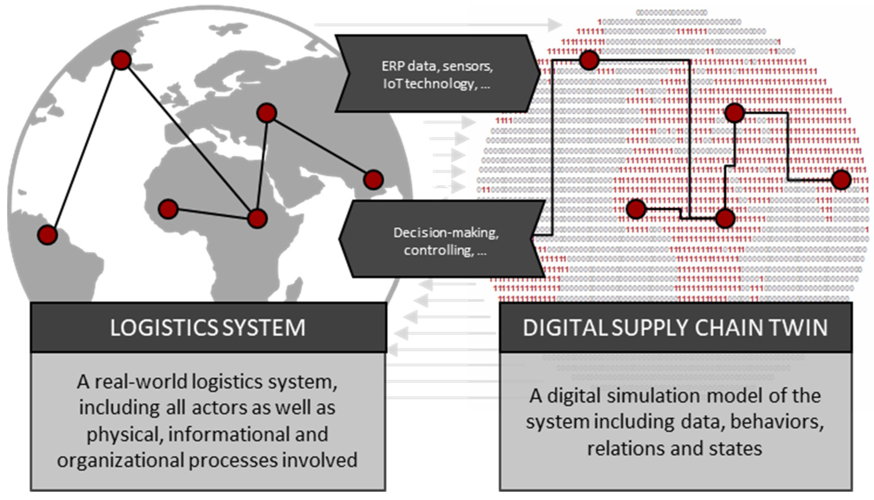
Figure 1 acts as a visual representation of the concept.
A digital logistics twin or digital supply chain twin (DSCT) is a digital dynamic simulation model of a real-world logistics system, which features a long-term, bidirectional and timely data-link to that system. The logistics system in question may take the form of a whole value network or a subsystem thereof.
Through observing the digital model, it is possible to acquire information about the real logistics system to draw conclusions, make decisions, and carry out actions in the real world. The DSCT enables the use of diagnostic, predictive and prescriptive methods with the ultimate goal of holistically improving the logistics performance along the whole customer order process [
2].
Among other aspects, the authors underline the importance of dynamic simulation capabilities in a DSCT, which in turn enable the user to run what-if scenarios. It is also made clear, that not all attributes of a DSCT are predefined when talking about the general concept. While some DSCTs are updated in real-time, for example, for others a lower updating frequency is sufficient. These attributes are determined by the specific use case, in which the DSCT creates benefits.
In the study at hand, a DSCT on the network-level is analyzed. It is applied in the area of network management, more exactly multi-echelon inventory management. In multi-echelon inventory management, the DSCT represents a SC from suppliers to customers. This model is then used to test inventory and procurement strategies and evaluate their SC performance [
2]. In this sense, the DSCT might also be used to improve a company’s ability to react to SC disruptions and other risks in order to improve SC resilience [
12]. In order to do so, the DSCT is updated in a timely manner. Real-time updating seems to be unnecessary, because relevant changes in the system do not occur within seconds or minutes. SC disruptions may be addressed in day-to-day operations, where the user is still able to respond efficiently. Therefore, a daily frequency seems to be sufficient. A DSCT might be used both reactively and proactively. Some SC disruptions, such as demand spikes, can be anticipated before they occur. In this case, scenarios can be proactively simulated in the DSCT in order to test the best possible response [
13]. In other cases, risks are not predictable. The DSCT then helps to make reactive decisions immediately after the incident occurs. In this study, only reactive use is examined.
Several researchers have addressed the use of a DSCT in the food industry. Defraeye et al. [
14] describe the optimization of a fruit SC by modeling the temperature of a transcontinental value network. DSCTs are considered a useful addition in the perishable food sector to minimize food losses due to improper storage. Burgos and Ivanov [
15] develop a model of a DSCT in risk management using the COVID-19 pandemic as a motivation, as it can help value networks recover after a breakdown. AnyLogistix (ALX) is used as a simulation tool. However, their approach notably lacks the feedback of the DSCT into company processes and therefore does not differ significantly from a basic SC simulation model. Nikitina et al. [
12] develop a DSCT of a food network with the help of a mathematical simulation model. The complex properties of the food products play a decisive role in their calculations.
In recent years, FSCs have been subject to numerous simulation studies, observing their ability to react to SC disruptions. Lohmer et al. [
16] analyzed different resilience strategies with an emphasis on blockchain technology. Singh et al. [
17] as well as Zhu and Krikke [
18] examined the effects of COVID-19 related disruptions on FSCs. All these studies underline the importance of resilience enhancing technologies to ensure SC performance even in the face of SC disruptions. Accordingly, Yuan et al. [
19] stress the importance of horizontal logistics collaboration. This study builds on this area of research by examining the use of DSCTs to improve decision making in FSCs in the face of SC disruptions.
The results of this study will tie in with various studies in DSCT research. First, the organic food industry is identified as a relevant industry for the use of a DSCT by Srai et al. [
7], as it promises higher transparency. Moreover, a continuation of some aspects of the publication by Burgos and Ivanov [
15] is given, in which the authors perform scenario analyses using a simulation model of an FSC. This study further developed their approach by extending the quantification method to integrate a feedback loop into the real logistics system. Finally, Gerlach et al. [
2] identified a research gap in quantifying DSCT use. Accordingly, through the investigation of a DSCT in the organic food industry conducted in this study, insights can be derived that have not yet been addressed in academia.
This study seeks to further investigate the use of DSCTs in the organic food industry. Therefore, a case study featuring an organic FSC was constructed, which will be described in detail in the next section.
2.2. A Case Study in Organic Food Supply Chains
In this study, subject of investigation is a SC in the organic food industry. Organic food products are usually available in conventional retail supermarkets as well as in organic supermarkets, in which up to 10,000 different organic food articles can be found. Often, the procurement is carried out regionally in small-scale and decentralized transports [
8]. The FSC is one of the most complex and fragmented value networks, with production mostly worldwide. The wide range of products and the large number of individual product categories lead to a variety of logistical challenges. Products such as dairy products, fresh meat, fish, fruit and vegetables or frozen foods must be temperature-controlled [
20]. This complexity is a further argument for the use of a DSCT.
Figure 2 shows the individual actors and functional areas of an FSC.
In 2021, Patidar et al. [
22] conducted a structured review of the literature published on FSC management in the past 15 years to give an overview of the research field and identify research gaps. Among other implications, the authors found that even though a large number of articles discussed and highlighted the problems, challenges, and issues in the FSC, few studies presented strategies to overcome them. Especially the prevention of food loss through LSCM efficiency as well as the proper utilization of emerging technologies are identified as possible research gaps. This work aims at filling these gaps by examining the DSCT as a potential technological solution in the context of a domain-specific case study.
The case study examined in this work features a European FSC, with an emphasis on the German sales market. It includes a value network from suppliers to supermarkets (retail stores). Even though production takes place worldwide, the immediate suppliers of finished products are located in Europe, predominantly in Germany. There are twelve European suppliers, who receive their products from global producers. These suppliers supply a central distribution center (DC) in Germany, which in turn supplies five wholesalers, that are spread across Germany. These sites act as hubs, storing goods and distributing them to the retail stores all across the country. The retail stores are characterized as organic food supermarkets and act as the final customer for the FSC in question. Hence, the system in question is a four-stage value network. Only four product categories are considered.
Figure 3 shows a simplified representation of the FSC.
The case study company sells organic food produce at German retail stores. It is based on one of the three largest retailers in Germany, which sources about 6000 organic products worldwide [
23]. In order to achieve greater visibility and transparency along the FSC, the company decides to use a DSCT. It hopes to be able to better manage its network-wide inventory as well as react to SC risks operationally and strategically.
The user of the DSCT is the SC manager in Germany, who coordinates and optimizes the company’s network-wide product supply. She is responsible for the procurement of products, up to the delivery of the products to the supermarkets. His tasks include developing procurement, inventory and order strategies, drawing up contingency plans and evaluating suppliers. The SC manager sits at the DC but is in close contact with dispatchers in the respective hubs, in order to optimize inventory levels across different SC echelons. One of the user’s goals is to ensure efficient hub utilization, enabling timely product deliveries to the retail stores, even under changing SC conditions. The scope of the SC manager in this case study thus includes both operational and strategic tasks. Accordingly, she is responsible for procurement logistics, determining the ordering policies as well as defining inventory policies. Thus, a holistic approach to LSCM tasks is given [
24].
The user in question has access to a network-wide DSCT, representing the SC from the suppliers to the retail stores. In the event of changing SC conditions, he can run “what-if” scenarios in order to develop a suitable strategy. For this purpose, it is assumed that the user feeds the knowledge gained back into the real logistics system by adopting different strategies. The DSCT evaluates these strategies across different dimensions of SC performance. For this purpose, several performance measurement systems exist in theory and practice, which include financial as well as non-financial measures [
25,
26].
2.3. A Quantification Method for DSCT Benefits
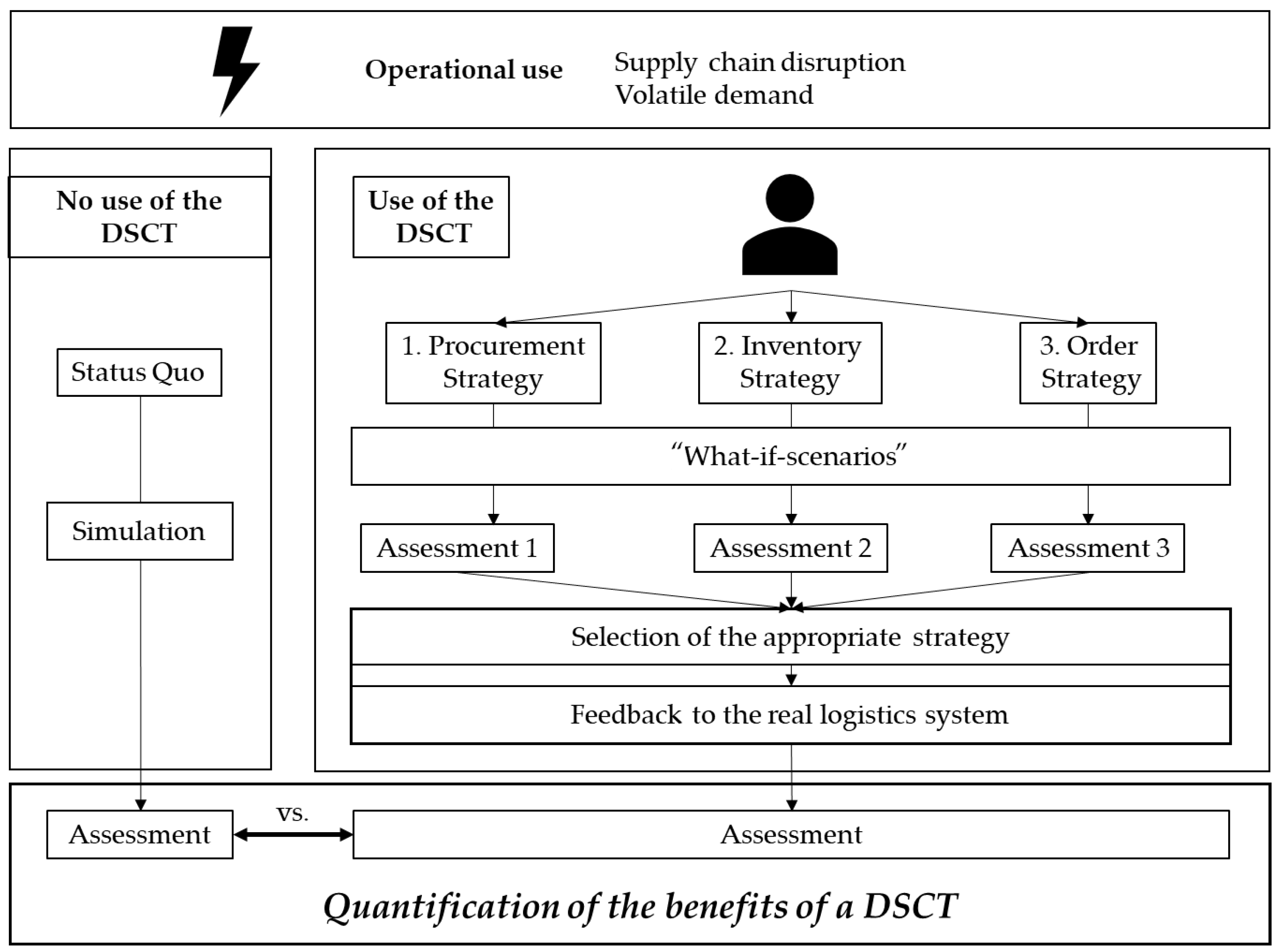
Ironically enough, most DSCT studies do not feature a real-world DSCT. They mostly use a basic simulation model, which is not connected to any real-world system and therefore does not qualify as a DSCT. Still, it is carried out so in a variety of studies: A SC disruption is first being simulated, after which the level of SC performance drops. Subsequently, the features of the simulation model are being used to improve SC performance due to strategies, that better fit the new situation. The level of improvement is then presented as the expected benefit of the DSCT.
However, this approach neglects the fact, that in a real use case a user would have to use the DSCT during ongoing operations. There has to be a feedback loop returning the simulation results into company processes. This process needs to be emulated in order to obtain a better understanding of the effect a DSCT use has on SC performance. Even if this feedback loop is not executed using real-world company data, it can be emulated using a fitting simulation model. For this purpose, an adequate method should be developed in order to be able to adequately quantify the benefits of using a DSCT, as a basic simulation model is not sufficient. Therefore, in accordance with RO1, the following approach is presented as a possible solution:
Use Case Definition
Scenario Selection
Baseline Scenario
Modified Scenarios
Process Emulation
System Simulation
Initial Baseline Scenario
Modified Baseline Scenarios
Optimized Modified Scenarios
Use case definition: First, the DSCT use case is to be defined in detail. This begins with a description of the logistics system in question. Furthermore, the input and output parameters have to be set. The input parameters consist of the decisions and actions that the user in question inputs into the real system. The output parameters are certain LSCM performance measures. The user’s performance is evaluated on the basis of these. The measures used should always form a holistic performance evaluation of the logistics system in question, as is appropriate in LSCM.
Scenario selection: Next, scenarios to be investigated are to be selected. The scenarios chosen should reflect possible applications of the DSCT in the use case described prior. The first scenario should always be an initial baseline scenario. On the one hand, this initial baseline is used as a validation. The output parameters should be compared with real-world measures to ensure model accuracy. On the other hand, the initial baseline serves as a means of comparison. Afterwards, the modified scenarios have to be selected. These scenarios should represent alternative situations the DSCT user can find himself in during ongoing operation. For this purpose, domain experts should be consulted. The scenarios should be both probable and relevant in terms of the use case in question. For an application in risk management, for example, these modified scenarios might be the occurrence of various SC risks.
Process emulation: The first level of simulation is the emulation of the user process. This should be a replication of all the steps a user would perform in the real-world optimization process. During this phase, the simulation model acts as a tool for reacting to the modified scenarios defined in the prior step when trying to optimize the output parameters. For this purpose, objectives have to be defined. They may take the form of measures and respective target values the user tries to achieve with her actions. As the user would not have unlimited time in a real-world application, money and other resources, these resources also have to be defined beforehand. This may be carried out by setting a fixed maximum number of iterations for the optimization process.
System simulation: Ultimately, the different final scenarios have to be fed into the model to simulate the system’s behavior over time, thus forming the second level of simulation. During this phase, the simulation model acts as a tool to reflect the system’s behavior over time. For this purpose, the results of the prior process emulation step are taken. These results represent the user’s decisions that were made using the DSCT as a decision support tool. These decisions are then input into the simulation model in the form of altered input parameters. In order to be able to put the results into perspective, the initial baseline scenario should first be simulated. Subsequently, further baseline scenarios should follow—one for each modified scenario to be investigated. The results of these experiments reflect the system’s behavior when the modified scenarios occur, but no DSCT is used. Lastly, the optimized modified scenarios should be simulated. The results of these experiments reflect the system’s behavior when the modified scenarios occur and a DSCT is used to optimize the system. The input parameters for these experiments are taken from the process emulation step. The reaction time of a user should also be considered in this step.
Following these steps should give a realistic overview of the expected benefits of using a DSCT in a given use case. A comparison between the initial baseline scenario and the modified baseline scenarios gives an estimate of the expected outcomes of the SC modifications on SC performance. In the example of risk management, this may form a means of risk assessment. A comparison between the modified baseline scenarios and the optimized modified scenarios gives an estimate of the effect DSCT use has on LSCM performance regarding the use case in question. In the following, the method was applied to the use case of this study:
Use case definition: The use case in question is multi-echelon inventory management of an FSC. A detailed use case description is presented in
Section 2.2. The input parameters are the inventory, procurement, and order strategies of the DC and the hubs as described in the case study. In order to evaluate the DSCT’s effect on SC performance, a fitting performance measurement system was derived from theory. The performance measurement system is divided into the five categories of efficiency, flexibility, responsiveness, food quality and sustainability [
25,
26,
27]. Each category is measured by key performance indicators (KPI) that are presented in
Table 1:
Scenario selection: As the use case in question deals with multi-echelon inventory management of volatile SC, the scenarios to be examined are different volatility scenarios. Three scenarios including two different kinds of SC disruptions were examined. First, an increase in demand. Second, the breakdown of a supplier. Third, both a demand increase and a supplier breakdown.
Process emulation: The user utilized a simulation model in order to test different strategies in response to SC disruptions. Therefore, he ran experiments for different what-if-scenarios with the DSCT and made quantitatively justified decisions on suitable solutions based on the experiment results. His ultimate goal was the optimization of the logistics system in the face of the given SC disruption. For reasons of simplicity, only one objective was defined for this study: Achieving a service level of at least 98% per product for all locations within the scope. Still, all SC performance measures were evaluated in the end. For resource constraints, a minimum of 5 iterations and a maximum of 15 iterations were selected. The what-if scenarios were carried out using a consistent procedure, which will be further described in
Section 3.3. This process led to a final set of strategies for each of the three volatility scenarios, determined by the user in order to best handle the given SC disruptions.
System simulation: In this step, the system’s behavior over time was simulated for each volatility scenario. For this purpose, the initial baseline, the modified baseline, and the optimized modified scenario were compared. Thus, the use of a DSCT in the given use case could be evaluated. A visual representation of the applied method is shown in
Figure 4.
3. Research Design
In order to apply and test the developed method and its application to the given use case, a simulation study was conducted. ALX was used as a simulation tool. Furthermore, a well-proven process model for conducting simulation studies by Rabe et al. [
28] was used as a methodological guideline. The sub-processes of said model were slightly adapted and are described in the following part. Similar approaches have been utilized in the recent scientific literature, where simulation studies were chosen as a methodology in order to examine the effects on organizational or technological measures on FSC performance [
16,
17,
18,
19,
29].
3.1. Objectives and Tasks
Objective description: The objective of the simulation study is quantifying the effects of using a DSCT for managing inventory and procurement in an organic FSC. Simulation is used as it constitutes a major component of the DSCT. Thus, this simulation study directly targets RO2.
Task description: The objective is met through conducting what-if scenarios, emulating the use of a DSCT in the face of different volatility scenarios. The selection of the volatility scenarios is further described in
Section 3.3. The effects of different strategies on certain LSCM measures are then evaluated in order for them to be comparable. Therefore, the user performs an optimization for each volatility scenario in order to deal with the DC disruption she is facing. By means of dynamic factor design, a step-by-step attempt is made to improve LSCM performance.
3.2. System Analysis and Model Formalization
The system in question is the FSC described in
Section 2.2, with focus on four product categories: fruits, vegetables, meat, and fish. For reasons of simplicity and feasibility, a consideration of sub-categories or single products was refrained from. To gain insights into the system, several data sources were used. Some of the data used were freely available on the Internet, while other data were obtained from publications. These are either statistical calculations, real data, or estimates. All data sources are provided in the following paragraph.
The location data regarding the retail stores in Germany were taken from a publicly available database [
30]. The demand values of the individual product categories are based on a calculation using the per capita consumption per year with the respective market share of the given retail chain. This was then multiplied by the share of organic food in the total food market in Germany. Therefore, the demand per day per inhabitant in Germany was determined. Finally, the demand of all retail stores was automatically generated in ALX, using the number of inhabitants of the different locations [
23]. The sales prices were determined by the average prices of the given food categories in the year 2022 [
9].
For reasons of simplicity, shipping costs were included in the purchase price. Initial stock levels as well as costs for stock refilling were also reflected in the purchase price. [
15] To measure CO
2 emissions, truck emission factors based on load weight and distance travelled were derived using the publicly available EcoTransit calculation tool, which is recognized in research. In order to take energy consumption for truck loading activities into consideration, an additional coefficient was added per delivery [
31]. Furthermore, a distance- and weight-based calculation of travel costs was selected.
Since only some product categories are included, the key figure of truck utilization is not decisive. Accordingly, trucks could drive at less-than-truck-load (LTL) between locations. Two types of trucks were considered. Between the suppliers, the DC and the hubs, trucks with larger capacity (26 t) were used. The last-mile delivery to the supermarkets was executed using trucks with smaller capacity (7.5 t), as they have to drive to city centers.
Inventory policies of the DC and the hubs were set to be identical: make-to-stock (MTS). By selecting a Min-max policy (s, S), excessively high and low inventories can be avoided. For this purpose, a replenishment point (s) and a target stock (S) were defined. A new order is placed whenever the inventory level falls below the replenishment point (s). The ordered quantity is the delta between S and the current inventory level. The target stock (S) at the DC was set to be larger than the daily demand in Germany as a whole. The replenishment point (s) at which reordering takes place is usually half of the value of S. At the hubs, inventory levels are lower. The target stock was set to be equal to the daily local demand per product. Inventory levels are checked twice a day, so that orders are placed a maximum of twice a day.
To calculate the system’s inventory cost, the storage costs at the DC and the hubs were calculated. The storage costs for the suppliers were not considered. All suppliers had the same capacity and could order from the producer as often as they wanted. The expected lead time of the retail stores was set to be two. An overview of the case characterization is presented in
Table 2, while
Figure 5 shows the model SC implemented in ALX.
3.3. Experiment Plan and Analysis
Four different kinds of scenarios were tested in order to simulate the system’s behavior in the face of different forms of SC volatility. There is one initial baseline scenario and three volatility scenarios. In the initial baseline scenario, the status quo of the FSC was simulated. In this scenario, the FSC was set up so that all suppliers are available and deliver to the DC in Lorsch. The SC performance measurement system presented in
Section 2.3 was used to evaluate LSCM performance. It should be noted that some of the KPIs have different names when implemented in ALX. The dropped orders, for example, were derived from the product backlog measured in the simulation tool, as both measures represent the lack of order fulfillment to the customer.
Scenario 1 examines the occurrence of a customer risk. One reason for this could be a worldwide pandemic, for example, which causes a strong and spontaneous increase in demand. It was assumed that demand increased by 100% during a defined period. The duration of the demand increase was set between 15 and 120 days. In a sensitivity analysis, the influence of the duration of the demand increase was determined first.
In scenario 2, there are supplier disruptions. The suppliers of meat products in Germany close their sites and can no longer supply the DC. The company needs to react quickly and use the DSCT to develop a strategy to still be able to supply the retail stores. The breakdown duration was set between 15 and 90 days. Again, a sensitivity analysis was performed to evaluate the effect of different durations of supplier downtime on the LSCM performance.
In scenario 3, it is assumed that both effects mentioned above occur simultaneously. Possible reasons for this are global pandemics causing unexpected demand spikes and factory closures. The duration of both the demand increase and the supplier breakdown was assumed to be 60 days. The magnitude of the demand increase was set between 50% and 200%. Again, a sensitivity analysis of different magnitudes of demand increase was performed.
An overview of the different scenarios and the respective experiments is presented in
Table 3.
For each scenario, the SC performance measurement system presented in
Section 2.3 was used to evaluate different inventory and procurement strategies. The system was implemented in ALX in the form of a dashboard, which is a good representation of an actual DSCT being deployed in a real-world use case. For reasons of readability, not all parts of the dashboard can be shown in all steps.
For each scenario, the user then performed an optimization in order to deal with the DC disruption she is facing. By means of dynamic factor design, a step-by-step attempt was made to improve LSCM performance. A maximum of 15 iterations were conducted per scenario, with the goal of achieving a service level of at least 98%.
4. Results
In this section, the experiment results are presented. The section is structured in accordance with the different volatility scenarios presented in the previous section. For each volatility scenario, an overview of the LSCM performance is given. Additionally, a description of the disruption effects on the FSC is given in scenarios 1–3. Subsequently, the effects of the DSCT use are described. This is done not only in terms of LSCM performance measures, but also in terms of the system’s behavior over time.
4.1. Scenario 0: Initial Baseline Scenario
First, the initial baseline scenario was examined. For this purpose, one simulation experiment was conducted. The KPIs measured present the status quo of the FSC without any SC disruptions.
The lead time for each order is less than 0.54 days, the service level for each product is 100% at all times, and the available inventory in the hubs and the central DC is constant. Furthermore, there are no delayed or dropped orders. This overview reflects a functioning and efficient logistics system.
Figure 6 shows an overview of some important KPIs in the form of a dashboard. This dashboard represents the simulation tool, which is available to the real-world user for decision-making support.
The complete performance evaluation of scenario 0 is presented in
Table 4.
In the efficiency category, the total costs are about €309 million. Of this, 86% is attributable to purchasing costs, while 13% is attributable to inventory carrying costs and less than 1% to transport costs. This leaves an overall profit of €42.16 million, which accounts for approximately 13% of total revenue. The purchasing costs of 86% are rather high. However, this corresponds to the common share in the organic food industry, since the products are not being produced, but rather procured. In addition, other cost components are included in this amount, as described in the model assumptions in
Section 3.2.
It is observed that all orders can be delivered on time and that there are no dropped orders at any time. The fill rate is 100% and the average lead time is 0.32 days. Therefore, the logistics system can meet the retail stores’ lead time requirement of less than two days at all times. The service level per location and per product category is 100%. The average stock level per day is 281,159 kg. Accordingly, the DC and hubs are always ready to meet the customer demand. The total CO2 emissions from transport and storage are 4856 t CO2.
This evaluation acts a mean of comparison for the scenarios to come.
4.2. Scenario 1: Demand Increase
Disruption effects: After a demand increase occurs, some orders can no longer be fulfilled. Moreover, some orders cannot be fulfilled on time. This is reflected in the occurrence of dropped orders, as well as in the OTD and service level drop. As demand at the retail stores increases, demand at the hubs and at the DC in Lorsch also increases during this period. As a result, inventory levels in the hubs drop sharply, while the inventory level in the DC increases. The DC is supplied by several suppliers who normally do not use their maximum delivery capacity. The bullwhip effect is evident here, as the inventory fluctuation, that begins at the retail stores, is highest at the supplier level. After inventory levels in the hubs plummet, it takes a while for service levels to recover.
Figure 7 provides an overview of the disruption effects on the KPIs over time for different durations of demand increase. It shows a visualization of four important KPIs for two consecutive iterations. A sensitivity analysis shows that the longer the demand increase, the longer the average lead times. Furthermore, a linear relationship is observed between the duration of the demand increase and the effects described above. The longer an increase lasts, the longer the logistics system takes to recover. This figure compares an increase of 30 and 60 days. More iterations have been made subsequently, up to a duration of 120 days, thus ending the sensitivity analysis. As the analysis shows a linear relationship between the disruption duration and the effect, the duration can be chosen freely within the given range without affecting the interpretability of further results.
Iterative Optimization: After the sensitivity analysis, a duration of 60 days was selected as a modified baseline. In the event of a 60-day demand increase, the user tries to improve the LSCM performance through various adjustments.
Figure 8 contains the dashboard with the relevant KPIs, on the basis of which various measures are taken. By means of dynamic factor design, a step-by-step approach is made to improve LSCM performance. Three steps are selected representatively to show the iterative improvement. By adjusting the order frequency, the number of delayed orders can be significantly reduced (iteration 8). Next, the availability of new suppliers leads to an improvement in service levels and fewer orders are delivered late (iteration 10). Finally, an increase in inventory leads to less dropped orders and thus to a stabilization of service levels (iteration 13).
Performance evaluation: In the final iteration 13, order strategies as well as procurement and inventory strategies have been adjusted in order to better adapt the logistics system to the SC disruptions.
Table 5 gives an overview of the LSCM performance of scenario 1 with the use of a DSCT (optimized) and without (baseline). However, the user can only react to the increase in demand in a reactive way. Therefore, a delay is simulated between the occurrence of the SC disruption and the point at which the changes are implemented in the logistics system. This leads to delayed orders and a slightly higher lead time.
When comparing the scenario 1 baseline with the optimized final iteration, an overall increase in costs is observed. Still, there is an increase in profit of around €11.5 million. This is because after the demand increase, there are 548 dropped orders, which in turn lead to lost sales and therefore less revenue. With the use of a DSCT this can be prevented. The service level of 0.99 is also notably better than without DSCT use (0.84).
4.3. Scenario 2: Supplier Risk
Disruption effects: After a supplier breakdown occurs for one product category (meat), it is observed that the lead time for meat products grows significantly for the duration of the breakdown. Meat orders from the retail stores arrive constantly and they cannot be serviced. Therefore, dropped orders are observed, which lead to lost sales. Inventory levels in the DC and the hubs are lower and the service level for meat products decreases.
Figure 9 visualizes the effects described above. A sensitivity analysis analogue to scenario 1 is carried out. Iteration 2 (30-day supplier downtime) and iteration 3 (60-day supplier downtime) are displayed in the figure.
Iterative Optimization: After the sensitivity analysis, a duration of 60 days was selected as a modified baseline. The user has different strategies to follow in the event of a supplier breakdown. Since no suppliers are available in Germany, an attempt is made to involve suppliers from abroad. Adding a supplier from Poland has the effect that no more orders are delivered late. The inventory levels in the DC and the hubs can also be increased slightly. As a result, the service level improves (iteration 5). Adjusting the order frequency for meat products in the hubs and distribution center results in the supplier not being able to re-deliver quickly enough because they have limited capacity and their location is further away from the DC (iteration 7). Finally, establishing and selecting a supplier relationship in the Netherlands with the same capacity but with a shorter distance leads to a significant improvement in service level and other relevant KPIs as compared to prior iterations (iteration 9). In addition, the DSCT helps to determine that the supplier from the Netherlands is sufficient. The costs for establishing new supplier relationships are neglected. The effects of adjusting the strategies iteratively are shown in
Figure 10.
Performance evaluation: In scenario 2, the effects are similar to scenario 1. In the final iteration 9, order strategies as well as procurement and inventory strategies have been adjusted in order to better adapt the logistics system to the SC disruptions.
Table 6 gives an overview of the LSCM performance of scenario 2 with the use of a DSCT (optimized) and without (baseline). Again, the user can only react to the supplier breakdown in a reactive way. Therefore, a delay is simulated between the occurrence of the SC disruption and the point at which the changes are implemented in the logistics system. This again leads to a slightly higher lead time.
The profit increases by €8 million when using a DSCT relative to the scenario 2 baseline. This occurs due to higher revenue, although total costs increase by 9%. The increase in revenue is due to the prevention of almost 7800 dropped orders. The main drivers for the higher total costs are the higher inventory costs of 28% and the higher purchasing costs of 9%. The lead time is also significantly lower after optimization (0.32) as compared to the scenario 2 baseline (1.46).
4.4. Scenario 3: Customer and Supplier Risk
Disruption effects: In this scenario, both a demand increase and a supplier breakdown happened simultaneously for a duration of 60 days. Effects from both scenario 1 and scenario 2 can be observed. As the demand in some retail stores cannot be satisfied, dropped orders occur. The performance measures related to the product category affected by the supplier breakdown (meat) suffer particularly in this scenario. The service level drops, as well as inventory levels at the hubs. The effects on the KPIs are significantly higher than in the prior two scenarios, as the logistics system has to deal with two disruptions at the same time.
Figure 11 gives an overview of the observed effects.
Iterative optimization: After the sensitivity analysis, a demand increase of 100% was selected as a modified baseline. The user then again tries to handle the SC disruptions properly. The supplier breakdown is prioritized, as its impact is more severe when compared to the demand increase.
Figure 12 shows another exemplary excerpt of the user dashboard, where the inventory levels of the DC for different strategies are shown. In the first two visualizations, stock outs can be observed. In the last one the supplier selection seems to be appropriate, as no stock outs occur. This way the demand can be met.
Figure 13 shows some significant iterations in the optimization process. The addition of two suppliers stabilizes inventory levels in the DC. It also improves service levels and reduces the number of dropped orders (iteration 7). Increasing order frequency leads to higher inventory levels at the hubs as well as an improved service level (iteration 8). Finally, an adjusted inventory strategy leads to the required service level (iteration 14).
Performance evaluation: In scenario 3, it took the user 14 iterations to teach the final result. Order strategies as well as procurement and inventory strategies have been adjusted in order to better adapt the logistics system to the SC disruptions.
Table 7 gives an overview of the LSCM performance of scenario 3 with the use of a DSCT (optimized) and without (baseline). Again, the user can only react to the SC disruptions in a reactive way. Therefore, a delay is simulated between the occurrence of the SC disruptions and the point at which the changes are implemented in the logistics system. This leads to delayed orders and a slightly higher lead time and a reduced service level.
After optimization, the profit increases by €10 million. Even though the total costs increase by 21% due to the build-up of a higher inventory, the company is more profitable, since more than 8000 dropped orders can be prevented. The service level after the optimization (0.993) is significantly higher than without DSCT use (0.741).
5. Implications
This study shows how a DSCT can be used in multi-echelon inventory management of an organic FSC. A method for adequately measuring SC performance was developed and tested. When using this method as a guideline, one is able to not only make an estimation of the effects a DSCT in a certain use case has on LSCM performance, but also obtain a better idea of the user process during ongoing operations. Additionally, an analysis of the conducted case study gives a good overview of what benefits are to be expected when implementing a DSCT in a comparable use case in the food industry. This study is therefore of great use for researchers and practitioners alike who are concerned with DSCT.
The quantification method presented in
Section 2.3 generates multiple added values for DSCT research. First, it is a structured approach, which helps to generate reproducible and verifiable results when trying to measure DSCT benefits. Second, it displays some major advantages of using merely a simulation model for this purpose, which is still common practice as of today. By emulating and documenting the user process, a realistic application is ensured. Both the user’s objectives and the user’s resources are determined beforehand. Insights into the utility and usability of the DSCT can be obtained. Furthermore, a feedback loop of the optimization results into the logistics system is given. The user’s reactiveness is being simulated as well, thus creating a realistic overview of the system’s behavior in case of a real-world application. Lastly, the quantification method presents different levels of comparableness. Depending on what baseline is used, different conclusions can be drawn.
All in all, the quantification method is an improvement of the methods being used commonly in DSCT research. Therefore, when using this method as a guideline, researchers may be able to achieve more realistic and comprehensible results when trying to evaluate DSCT benefits. Practitioners may benefit from the method as well, as they may use it as an assessment tool when deciding on implementing a DSCT in their company. However, one has to keep in mind, that this study completely neglects the cost of DSCT implementation. In order to carry out a cost–benefit comparison, reasonable cost assumptions would have to be made beforehand.
The extensive simulation study conducted, which is described in
Section 3 and
Section 4, showed a realistic application of said method in a case study featuring an organic FSC. Thus, a first verification of the method is given. The organic food industry seems to be a plausible application domain. The volatility scenarios analyzed, namely demand increase and supplier breakdown, appear to be realistic scenarios, as they have been observed during the COVID-19 pandemic. For both scenarios, the DSCT presents itself as a feasible solution with promising effects on LSCM performance. An evaluation of the experiment results gives an estimate of the quantified benefits.
In case of a demand increase, a company’s profit goes down. This is because the logistics system is not able to fulfill the customers’ needs with the current order, inventory, and procurement strategies. Fill rate, service level, and OTD drop, while the lead time goes up. When a DSCT is used, these effects can be prevented for the most part. Notably, the logistics costs of the FSC go up, but since the revenue rises even more, an overall profit increase can be achieved, while otherwise quasi maintaining the LSCM performance level of the status quo. Interestingly enough, a comparison between the optimized scenario and the initial baseline shows, that a SC disruption in the form of a demand spike acts as both a risk and an opportunity, due to the potential profit gain for the company.
In case of a supplier breakdown, similar effects can be observed. It goes to show that if not properly dealt with, the missing supplier has devastating effects on the LSCM performance. Customer needs cannot be fulfilled and dropped orders go up, which in turn leads to a decrease in revenue. Other LSCM KPIs also deteriorate. When using a DSCT, a proper alternative for the missing supplier can be found, as is shown in the simulation experiments. Again, dropped orders can be prevented, resulting in higher revenue and therefore greater profit, while again maintaining the LSCM performance level of the status quo. Unlike in the event of a demand increase, the supplier breakdown leads to an overall profit loss when compared to the initial baseline. Still, the DSCT can help mitigating negative impacts, therefore potentially preventing major disasters.
These findings should present a first attempt of a realistic quantification method for DSCT benefits and make it easier for researchers and practitioners in LSCM to evaluate DSCT applications in practice. Combined with an adequate simulation study design, an assessment tool for DSCT implementation is formed.
6. Conclusions and Final Remarks
In conclusion, the aim of this paper was to develop a quantification method for evaluating DSCT benefits (RO1) and evaluate the effect of using a DSCT in multi-echelon inventory management of an organic FSC in terms of LSCM performance (RO2). All ROs have been met sufficiently by the authors.
Section 2.3 provides a conclusive method for benefit quantification of DSCT use. Meanwhile
Section 3 and
Section 4 describe the application of said method to a case study in the organic food sector, providing an evaluation of this very use case. Finally,
Section 5 derives implications for researchers and practitioners.
The quantification method presented in
Section 2.3 provides a conclusive process model for measuring DSCT benefits. This is of great value for practitioners with an interest in implementing a DSCT and DSCT researchers alike, since it paves the way for a reasonable cost–benefit comparison of DSCTs. As pointed out in
Section 5, the method features significant advantages over other methods commonly used in the field, most notably simple simulation models. This allows for more realistic DSCT studies, making the research field overall more tangible.
Furthermore, the results of the simulation study offer a first point of reference in terms of what benefits to expect when using a DSCT to improve decision making in an FSC. The use case in question featured decisions in regards to order, procurement, and inventory strategies in a multi-echelon logistics network when facing SC disruptions, namely demand spikes and supplier breakdowns. When utilizing the DSCT, the case study user was able to prevent the devastating effects the disruption would have had on LSCM performance. Through the application of better strategies, lost sales were prevented, resulting in higher company revenue. Even though these strategies sometimes led to increased costs, overall profit went up. Non-financial KPIs were also improved, leading to a better OTD rate, increased service levels, and overall shorter lead times. Nevertheless, these results have to be interpreted with caution, since validity and generalizability of the quantified magnitude of said effects heavily depend on the case study data quality. Since the case study at hand was constructed, the authors would like to refrain from deriving far-reaching implications for the food industry. However, the study results reveal insights into the underlying mechanisms at work in FSCs and how the application of a DSCT in this domain might look like.
Still, this study is not without limitations, which shall be addressed in the following paragraph. First of all, the simulation model used in this study does not classify as a DSCT, since it does not feature a data link to any real-world logistics system. So even though a real-world application process is being emulated, the level of accuracy of a DSCT cannot be matched. Therefore, some assumptions have been made while creating the case study and the respective simulation model. For one, truck utilization has mostly been neglected during evaluation, since only LTL transports have been used. This also led to higher CO2 emissions in the optimized scenarios. Since awareness for sustainability has been rising over the past years in LSCM, this factor should be subject of more detailed investigation in the future. Some costs and efforts have also been neglected during the modelling phase, for example the ones related to building supplier relationships and applying certain order strategies. Additionally, storage capacities were neglected for the DC and the hubs. Still, it was implicitly given through inventory costs. Lastly, it was assumed that the user does not take any actions in the modified baseline scenarios, that is, after the SC disruption occurs, but no DSCT is used. Given proper SC transparency, this seems rather unlikely. However, on the one hand, SC transparency might actually not be given, which would render the assumption somewhat realistic. On the other hand, the magnitude of the positive effects brought by the DSCT use are not crucial for the core findings of this paper. Therefore, even though the study results have to be put into perspective in this regard, the authors are nonetheless confident in the generalizability of this study’s results.
This work also lays the foundation for a variety of future research. Firstly, researchers may use the presented quantification method to more accurately evaluate DSCT benefits in their works. Secondly, as pointed out earlier, some dimensions of a LSCM performance have not been focus of this study. Especially the sustainability aspect of DSCT use should be looked into further. Thirdly, the application domain of the presented use case was the organic food industry. Similar studies should be conducted in other domains as well. Lastly, this study focusses solely on the benefits of a DSCT while ignoring the implementation costs for the most part. However, to properly conduct a cost–benefit evaluation, these implementation costs have to be estimated as well. Therefore, it seems crucial for researchers in the DSCT area to look into methods of evaluating DSCT implementation costs.
All in all, while benefits of using DSCT are widely being discussed in academia and practice, they are rarely quantified. As DSCT are a promising solution for handling complex tasks in LSCM, such as inventory and risk management, a detailed quantification of their effects on different LSCM performance measures is an essential instrument for making the concept’s discourse more comprehensive. The authors of this paper hope to have underlined the importance of this topic and also to provide guidance for researchers and managers who have an interest in the subject of DSCT.


