Structured Light Transmission under Free Space Jamming: An Enhanced Mode Identification and Signal-to-Jamming Ratio Estimation Using Machine Learning

Abstract

In this paper, we develop new classification and estimation algorithms in the context of free space optics (FSO) transmission. Firstly, a new classification algorithm is proposed to address efficiently the problem of identifying structured light modes under jamming effect. The proposed method exploits support vector machine (SVM) and the histogram of oriented gradients algorithm for the classification task within a specific range of signal-to-jamming ratio (SJR). The SVM model is trained and tested using experimental data generated using different modes of the structured light beam, including the 8-ary Laguerre Gaussian (LG), 8-ary superposition-LG, and 16-ary Hermite Gaussian (HG) formats. Secondly, a new algorithm is proposed using neural networks for the sake of predicting the value of SJR with promising results within the investigated range of values between −5 dB and 3 dB.

1. Introduction

Free space optics (FSO) plays a vital role in optical communications. FSO has many advantages like high bandwidth and low cost as it uses the free space as a medium to transfer an optical signal between transceivers; in addition, it enjoys the easiness of implementation compared to fiber-based communication systems. These advantages paved the road to incorporate FSO in modern life applications, including outdoor wireless access, storage area networks, last-mile access, enterprise connectivity, next-generation satellite networks, etc. [1,2].

Even with these advantages, FSO communications may experience some obstacles during signal transmission. Indeed, optical signals in free-space optics can be affected by many factors, examples of which include physical obstructions owing to the presence of physical objects, scintillation due to temperature variation, absorption caused by water particles existing in the air, and atmospheric turbulence and attenuation caused by weather changes such as the presence of fog, rain, or dust [3,4]. In addition, FSO is susceptible to human-made interventions, like optical signal interception or exposing light beam to a jamming source signal, in spite of the reliability of the overall system.

Jamming and environmental effects can be mitigated using different methods. For example, in [5], the authors used adaptive optics (AO) components to tackle the effect of atmospheric turbulence on the multiplexed Laguerre Gaussian (LG) mode data family, where an AO feedback closed loop is used as a pre- and post-compensation of weak and moderate turbulence. Another approach is by using conventional digital signal processing (DSP) techniques, instead of the costly hardware-based approaches. For instance, in [6,7], the authors used DSP to mitigate crosstalk-based turbulence in an emulated multiplexed LG modes propagation environment. A 15-tap 4 × 4 multi-input multi-output (MIMO) equalizer was used for four multiplexed LG channels, each carrying 20 Gbps quadrature phase-shift keying (QPSK) signal.

Recently, machine learning (ML) algorithms have been extensively used to tackle the problem of jamming and environmental effects in FSO signals. ML can be used to identify the modes of a structured light beam and provide a reliable estimate of channel parameters. For example, in [8], the authors used an artificial neural network to recognize the characteristic mode patterns of 16 different orbital-angular momentum (OAM) superposition modes, which are transmitted under the presence of strong turbulence conditions. Also, in [9], a six-layer convolutional neural network (CNN) has been proposed to identify LG and multiplexed LG modes under various turbulence effects. The multiplexed LG modes have shown a superior recognition performance over the conventional LG modes under severe turbulent channels. Besides, in [10], the persistent homology ML tool has been combined with CNN to enhance the recognition accuracy for decoding 16-ary LG and multiplexed LG modes transmitted in a turbulence environment. In [11], optimized multiplexed LG mode scenarios have been investigated using CNN and atmospheric turbulence. In [12], the authors exploited CNN for both estimating atmospheric turbulence and adaptive demodulation of 16-ary superposition LG modes in OAM-FSO communications. In [13], different ML algorithms like the k-nearest neighbor (KNN), support vector machine (SVM), and CNN are used to classify 8-, 16-, and 32-ary structured light beams under the presence of dust storm with different visibility ranges. In [14], the CNN was used to identify 8-ary LG modes, 8-ary of superposition LG modes, and 16-ary Hermite Gaussian (HG) modes of the light beam under jamming effect. Also, linear discriminant analysis (LDA) was used to determine the direction of arrival of the jamming signal. In [15], the CNN was used as an adaptive demodulator to enhance the performance of the wireless optical communication system. Moreover, the CNN was used to deal with underwater turbulence effects in underwater optical wireless communications such as water bubbles, temperature inhomogeneity, and water turbid [16].

This paper builds on the work of [14] to enhance the identification accuracy of a structured light mode of LG, superposition LG (Mux-LG), and HG beam structures under jamming effect. Although the results reported in [14] showed good performance in LG modes classification at signal-to-jamming ratio (SJR) of 1dB or higher, the classification accuracy was much lower at SJR of 0 dB or less. Similarly, the results achieved using Mux-LG and HG modes reached 100% at higher levels of SJR while they show degradation at SJR of −3 dB or less. Further, albeit the use of a powerful deep learning classifier (i.e., CNN), the classification results achieved at lower SJR were not as good as the results achieved at higher SJR over the three used modulation modes. Therefore, the current work is mainly concerned with two tasks. The first is the classification of structured beam modes, while the second is estimating the value of SJR. Specifically,

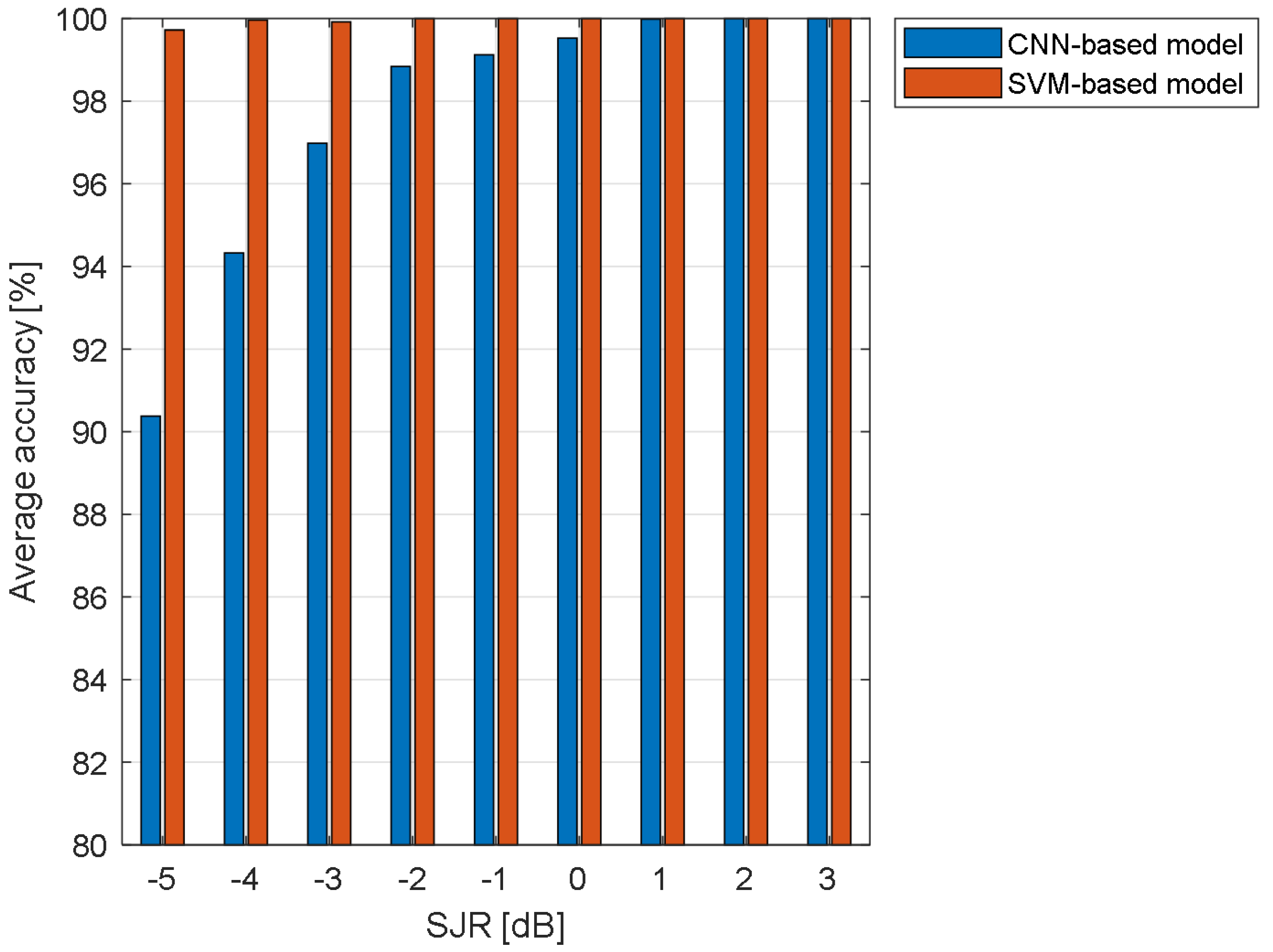
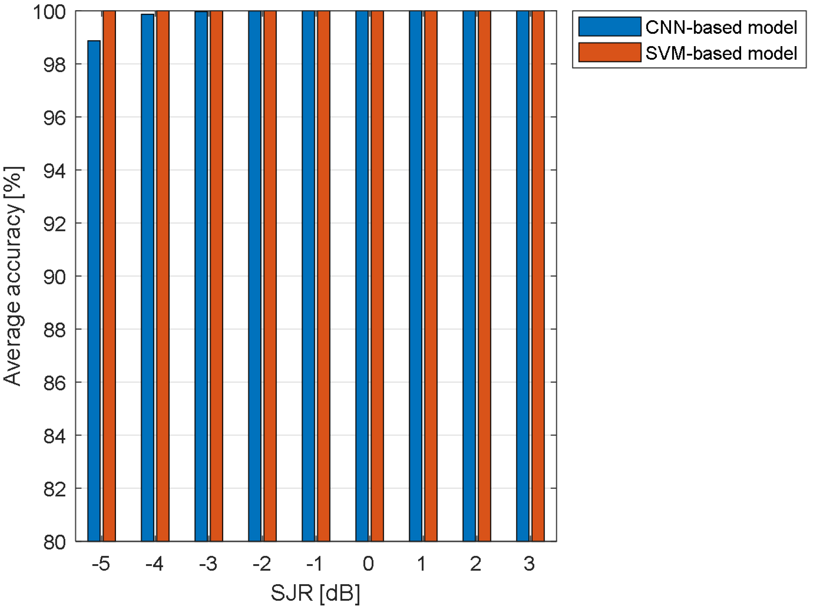
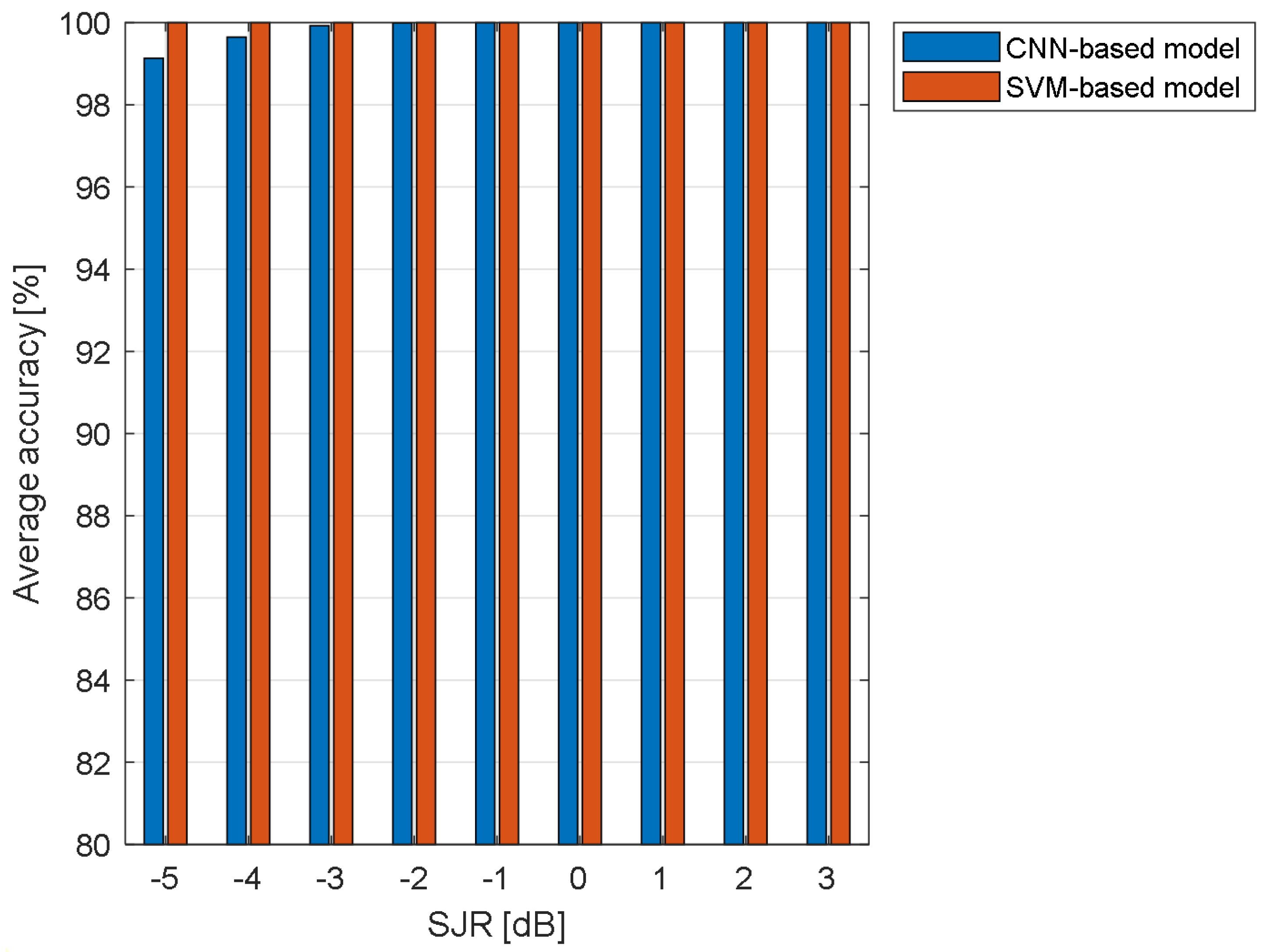
• A new method is proposed for augmenting the classification accuracy of light beam modes of LG, Mux-LG, and HG modulations. The proposed method is exploiting image processing techniques, which include image contrast enhancement using histogram equalization, followed by the histogram of oriented gradients (HOG) image descriptor to enhance the region of interest of the input images and to extract features. The HOG algorithm is heavily used in the field of computer vision as a preprocessing step. Furthermore, the proposed method uses the support vector machine (SVM), which is less complex compared to the CNN used in [14], to achieve the classification task. The proposed approach showed an excellent performance in the modes classification task, especially at low values of SJR (i.e., SJR $\le -3$ dB).
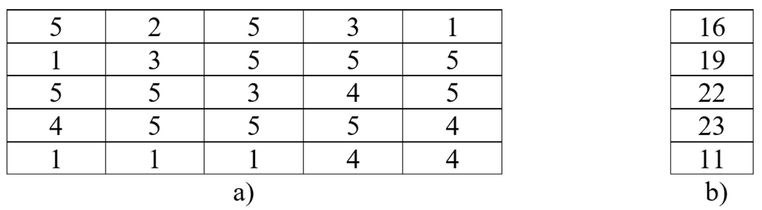
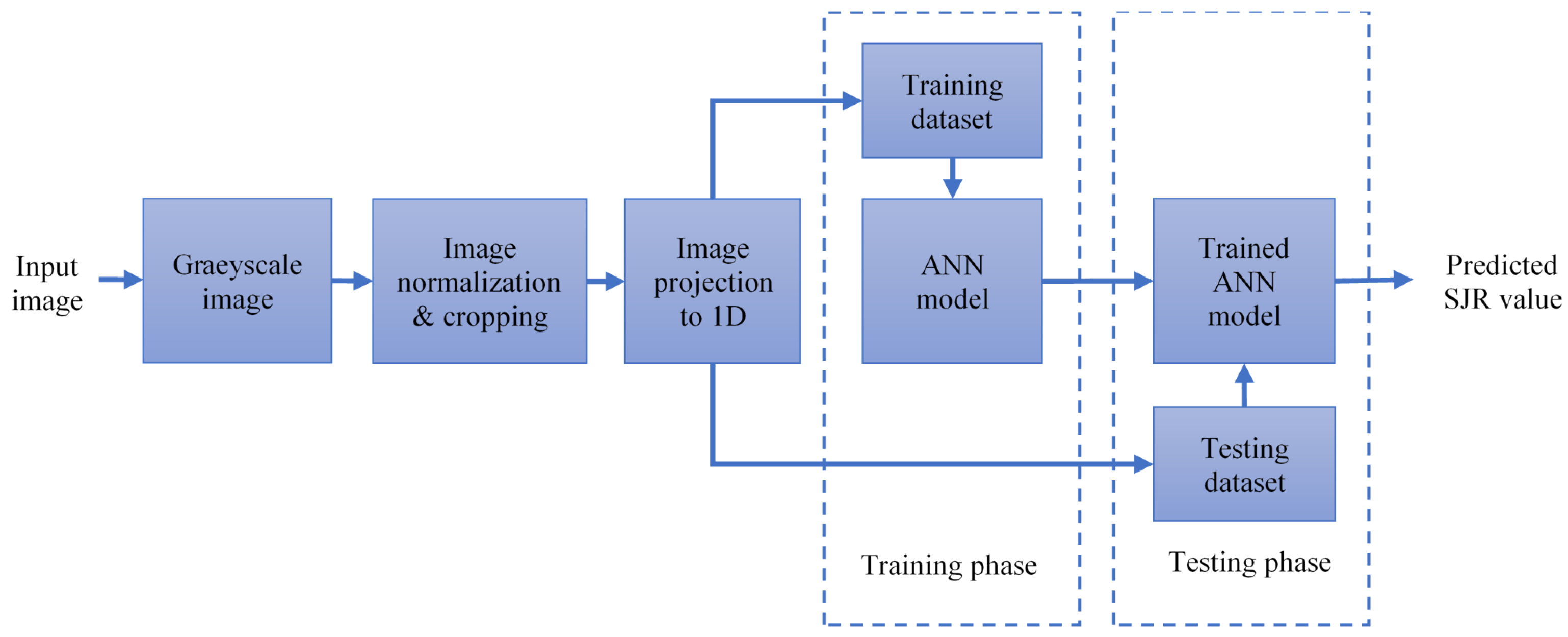
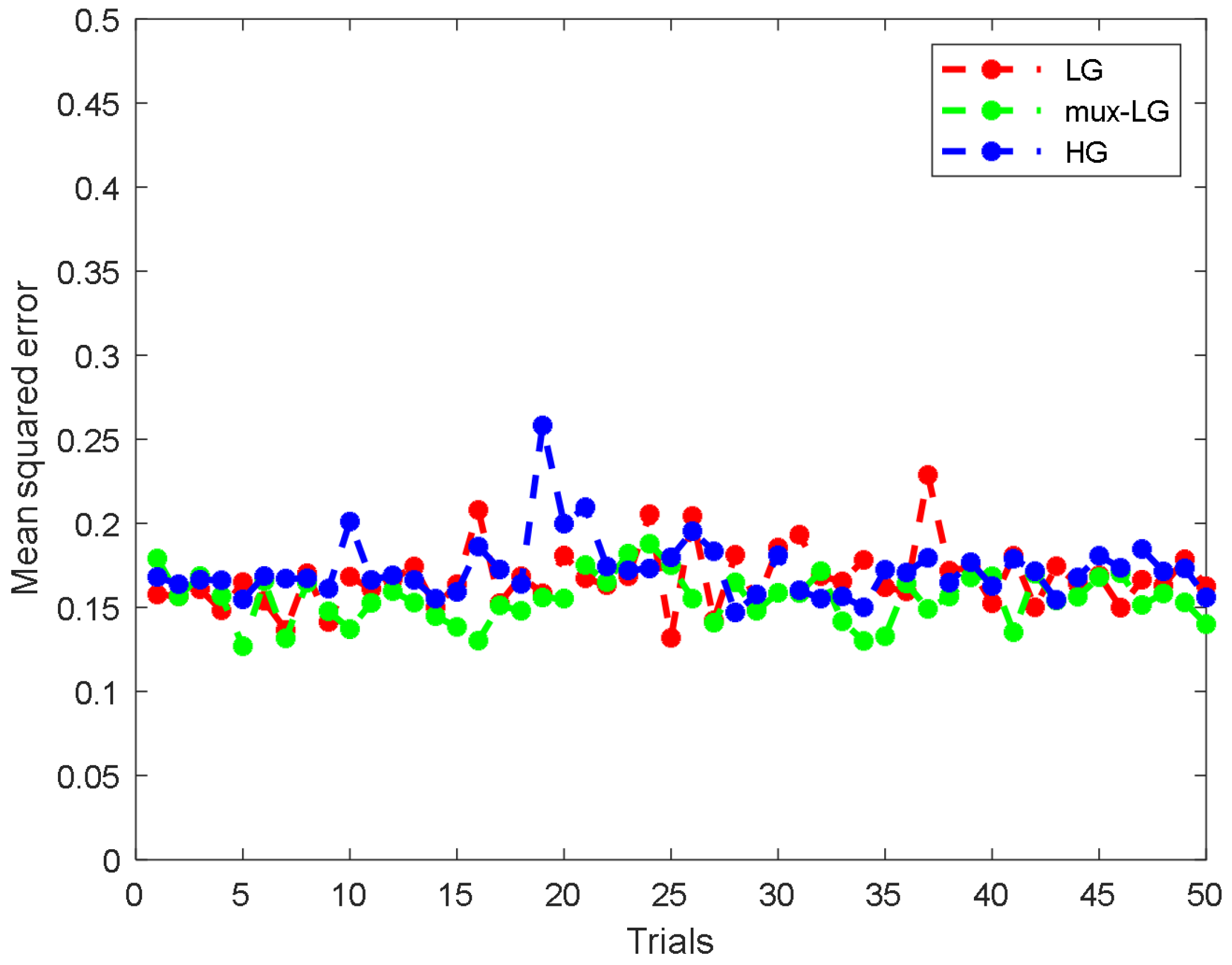
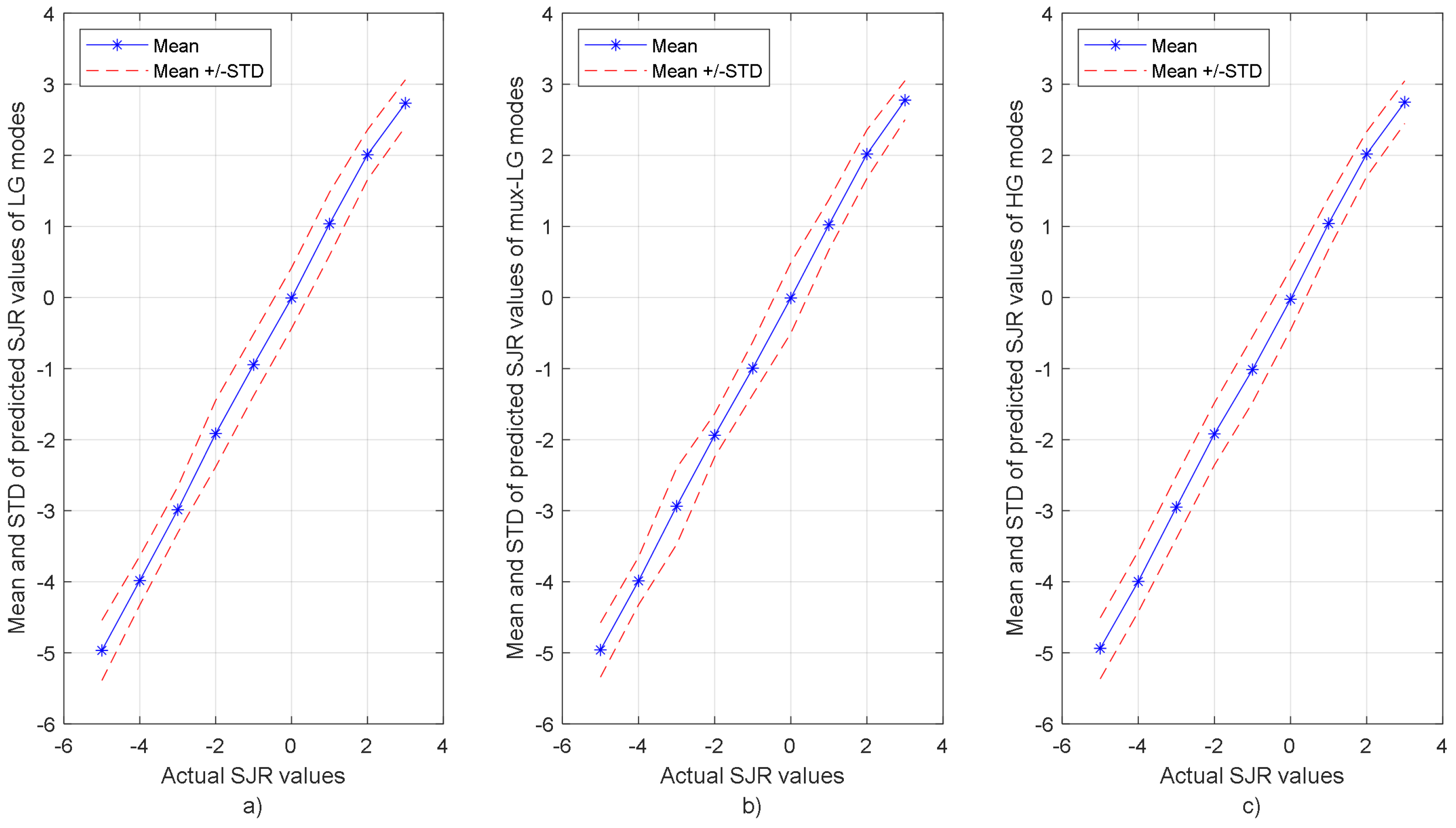
• A new approach is proposed to estimate the value of SJR from the received mode, to determine the level of jamming. This problem was not tackled in [14]. The proposed estimation method utilizes an image projection technique to extract features to be inputted to an artificial neural network (ANN). The proposed ANN model achieved a result with a mean squared error (MSE) of value less than 0.19 dB for estimating the SJR in the presence of the three different modulation modes.

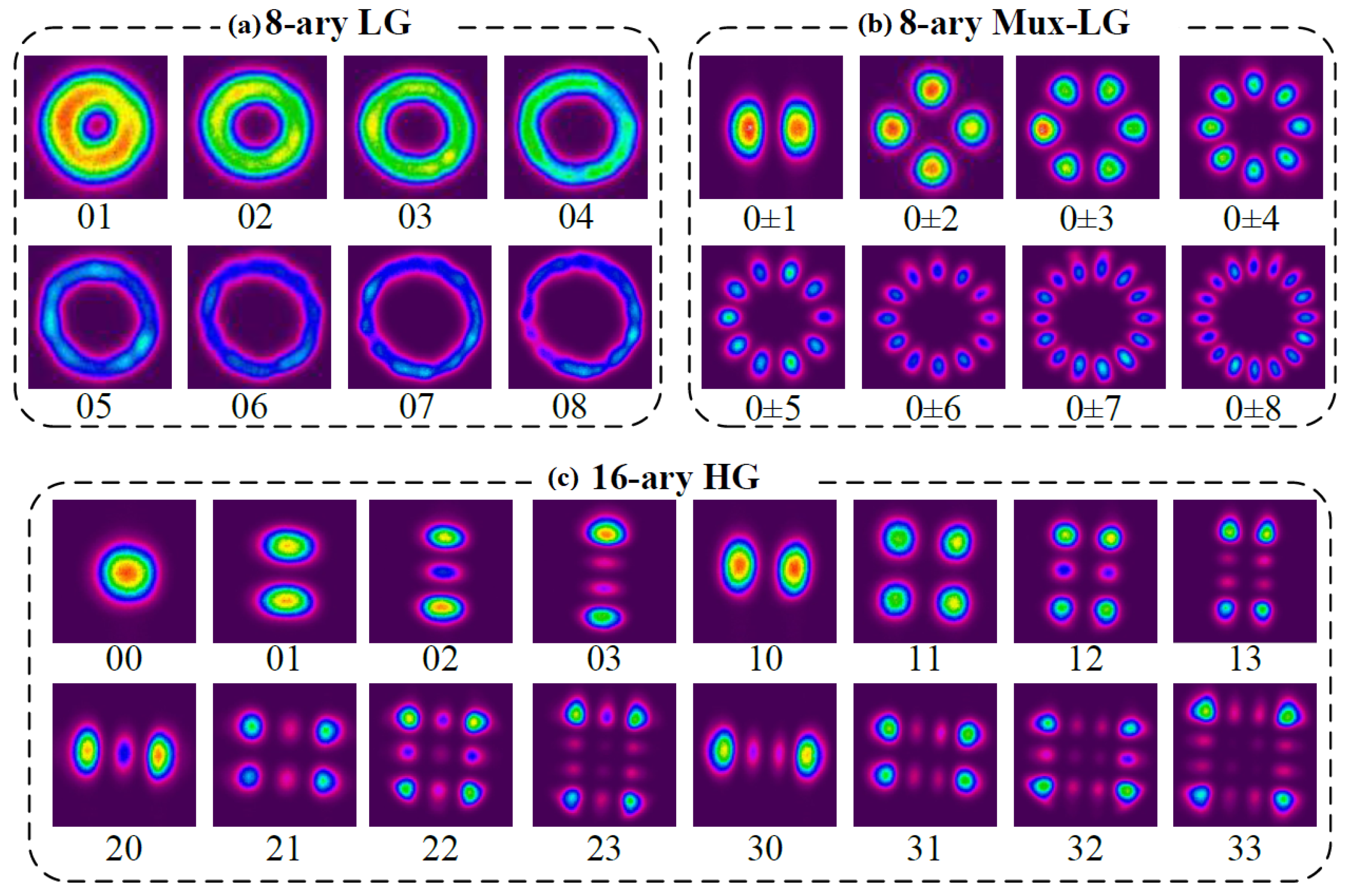
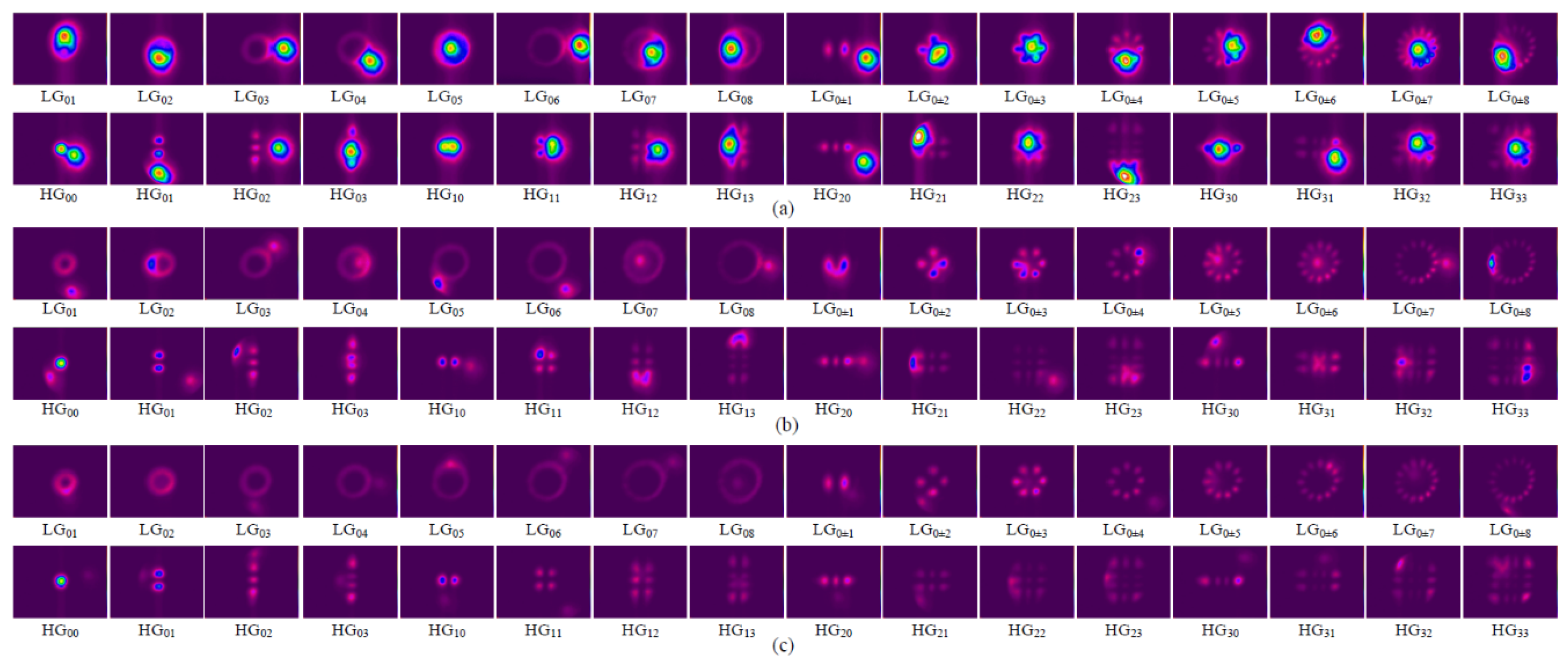
The results of modes classification and SJR value estimation are obtained using experimental data. In Section 2, more details about the utilized dataset are given. In Section 3, the proposed algorithm for modes classification is presented. Section 4 presents the proposed method for SJR estimation. Section 5 provides concluding remarks.

2. Dataset

The LG and HG mode families are considered to obtain three coding schemes as in [14]. The LG and HG mode families are solutions to the free space paraxial wave equation. The electric field of the LG and HG mode families in cylindrical $(r,\varphi ,z)$ and cartesian $(x,y,z)$ coordinate systems, respectively, can be written as [17]:

$$\begin{array}{cc}\hfill E_{(p,\ell )}^{LG}(r,\varphi ,z)=& \frac{1}{\omega \left(z\right)}\sqrt{\frac{2p!}{\pi (\mid \ell \mid +p)!}}exp\left[i(2p+\mid \ell \mid +1)\Phi \left(z\right)\right]{\left(\frac{\sqrt{2}r}{\omega \left(z\right)}\right)}^{\mid \ell \mid }\hfill \\ \hfill & \times L_p^{\mid \ell \mid }\left(\frac{2r^2}{\omega {\left(z\right)}^2}\right)exp\left(-\frac{ik{r}^2}{2R\left(z\right)}-\frac{-r^2}{\omega {\left(z\right)}^2}\right)exp\left(i\ell \varphi \right),\hfill \end{array}$$

(1)

and:

$$\begin{array}{cc}\hfill E_{(m,n)}^{HG}(x,y,z)& =\sqrt{\frac{2}{\pi n!m!}}{2}^{-\frac{n+m}{2}}exp\left[-i\frac{k(x^2+y^2)}{2R\left(z\right)}\right]exp[-i(n+m+1)]\hfill \\ \hfill & \times exp\left(-\frac{x^2+y^2}{{\omega }^2}\right)H_n\left(\frac{\sqrt{2}x}{\omega }\right)H_m\left(\frac{\sqrt{2}y}{\omega }\right),\hfill \end{array}$$

(2)

where ℓ and p are the azimuthal and radial indices of the LG mode, respectively. $H_n(.)$ and $H_m(.)$ are the Hermite polynomials of order n and m, respectively. $\omega \left(z\right)={\omega }_0\sqrt{1+{(z/z_R)}^2}$ is the beam spot size as a function of z, the beam waist ${\omega }_0$ and the Rayleigh size $z_R=\pi {\omega }_0^2/\lambda$ with $\lambda$ being the optical wavelength. $\Phi \left(z\right)=arctan(z/z_R)$ denotes the Gouy phase, $R\left(z\right)=z[1+{(z/z_R)}^2]$ is the beam curvature, and $L_p^{\mid \ell \mid }(.)$ are the generalized Laguerre polynomials [17].

Figure 1 shows the laboratory-generated beam profiles of LG, Mux-LG, and HG modes with no jamming interference. Here, the LG and Mux-LG modes were generated with a radial index (p) equal to zero and an azimuthal index (l) ranging from 1 to 8 and ±1 to ±8, respectively. It is worth noting that our investigations have focused on single-mode LG and Mux-LG twofold: (i) to compare the performance of the proposed identification method with the work done in [14]; and (ii) to test the jamming effect on beam structures that are widely used in literature [8,9,10,12]. However, other LG mode shapes can be obtained by considering a radial index greater than zero. This generates multi-ring LG modes [18]. By contrast, the HG modes shown in Figure 1c were generated for the m and n indices range from 0 to 3, considering all indices combinations. Figure 2 illustrates different samples of LG, Mux-LG, and HG modes with random wondering-around jamming effect at different values of SJR, that is −5, 0, and 3 dB. Here, Figure 2a,b show a strong and moderate jamming effect on the received mode. Whereas, Figure 2c illustrates a weak jamming behavior with distinguished received modes.

The LG, Mux-LG, and HG beam structures are experimentally generated, transmitted, and detected under the jamming effect with SJR ranges between −5 dB and 3 dB. This range has been selected as the modes with SJR < −5 dB are almost destroyed, and for values of SJR > 3 dB they have no noticeable jamming effect. Further, this range of SJR is consistent with the range considered in [14] to facilitate fair comparison. The LG and Mux-LG structures comprise 8 different modes, where each mode has 210 captured images at a given SJR. For the HG structures, there are 16 modes, with 210 images recorded for each SJR per mode. The data of this study is generated using a Teraxion continuous wave (CW) laser source operating at 1550 nm. The laser power was boosted to 20 dBm using an Erbium-doped fiber amplifier (EDFA). Then, the light is collimated, aligned, and modulated into LG, Mux-LG, and/or HG modes so that it can be sent through free space. A spatial light modulator from Hamamatsu was used to generate the three structured light signals. The generated light beam is exposed to a jamming source which is a standard Gaussian beam generated using another CW laser source working in the C-band with an output power varying from 8 to 15 dBm in order to adjust the SJRs. Both the original light beam and jamming signals are transmitted over a free-space link of 1-m inside the lab. These two signals are intercepted by a Thorlabs LB1471-C convex lens of 50 mm focal length and a charge-coupled device (CCD) detector (Ophir-Spiricon LBP2-IR2). Eventually, the captured intensity profiles of the different jammed modes are stored using a computer. Figure 3 illustrates a conceptual block diagram for the generation and measurements of light beams with jamming effect in the FSO framework.

3. Proposed Algorithm for Modes Classification

A successful OAM-based FSO communication needs to classify the received light modes for information retrieval. The 32-ary structured light beams, for example, can carry 5 information bis per mode. In this work, the proposed algorithm for modes classification consists of two main stages: (i) the preprocessing stage using image processing techniques, and (ii) the classification stage using ML.

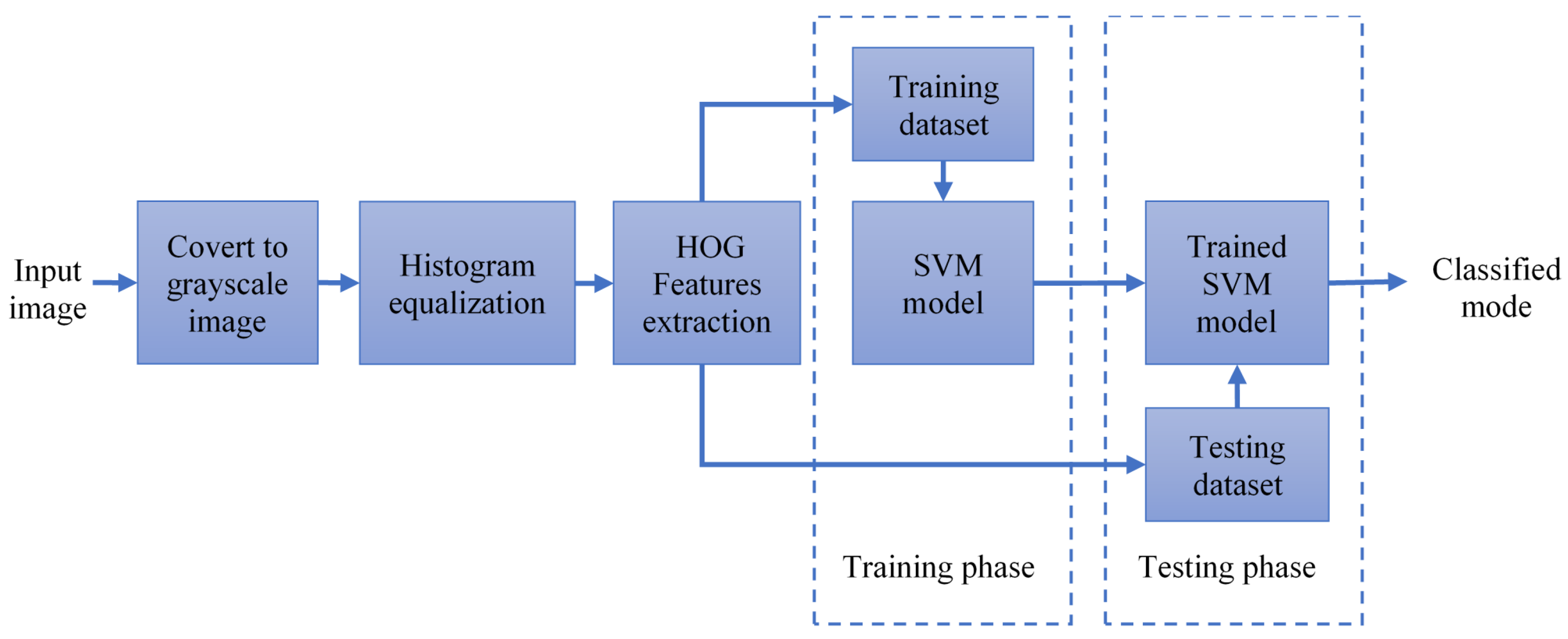
3.1. Preprocessing Operations

The experimental setup, described in Section 2, yields images of size 473 × 437 × 3 pixels. Examples of such images are shown in Figure 2. The first operation is to crop the region of interest of captured images to reduce their size to 245 × 270 × 3 pixels. Second, the cropped images are converted to grayscale images to reduce processing complexity. Third, the contrast between the background and foreground of a given image is enhanced through two main steps:

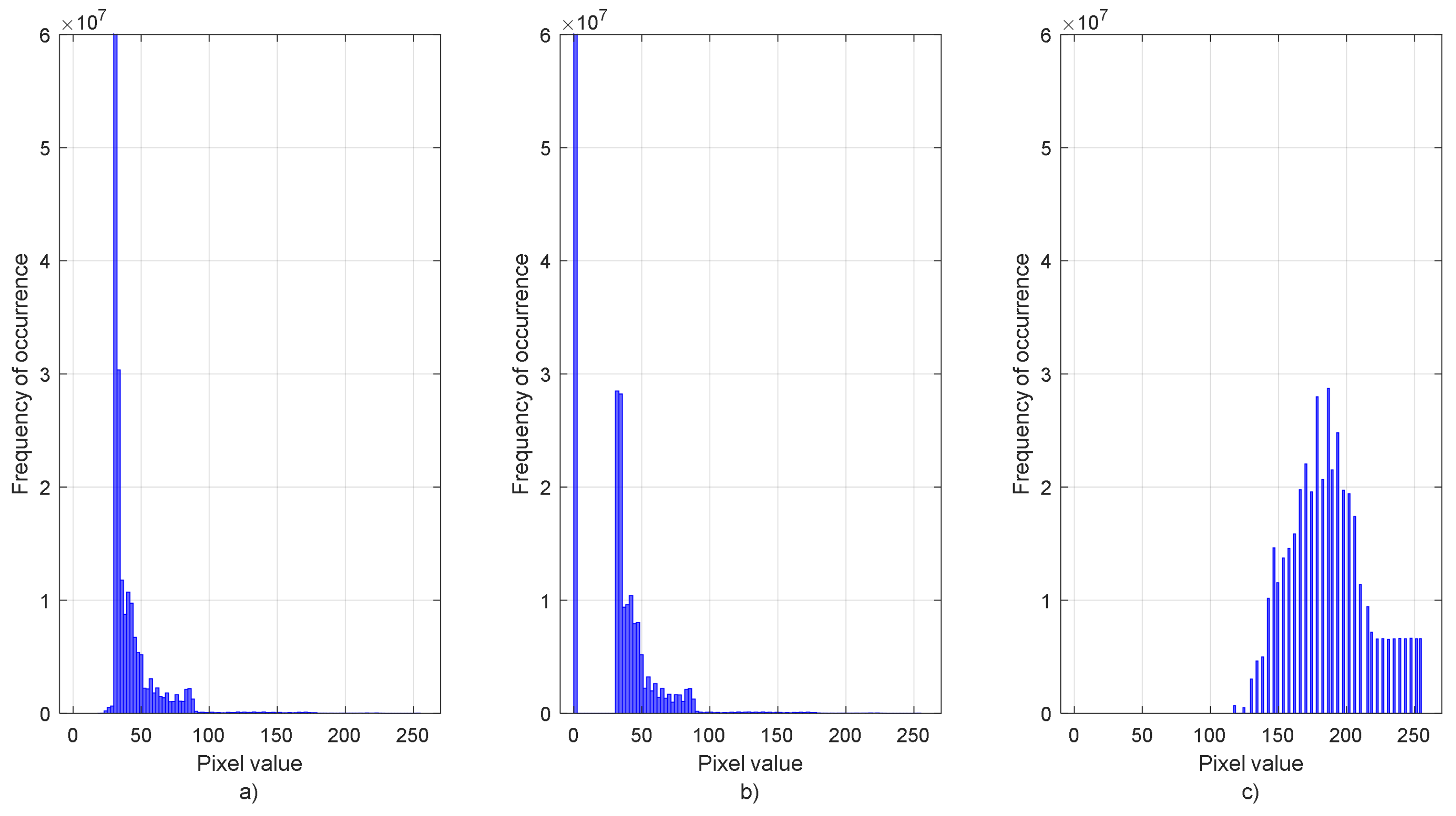
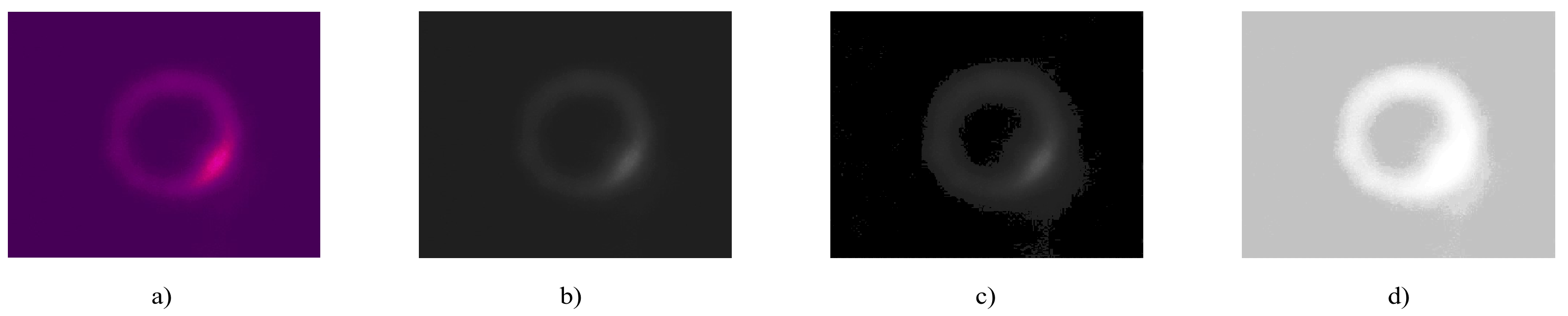
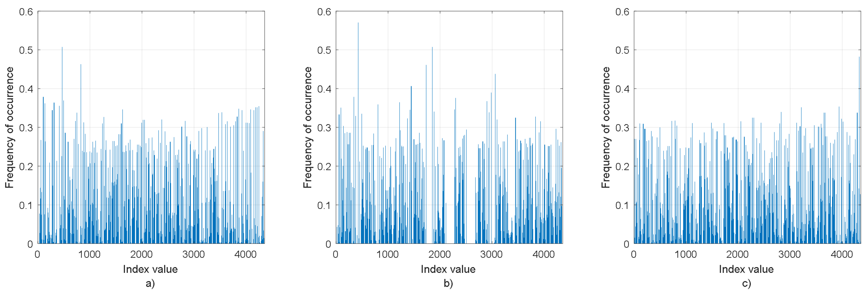
• Setting the intensity of background pixels to zero. The intensity of background pixels is obtained by computing the histogram of all images of the database, which is used for training the ML model. These images contain LG, Mux-LG, and HG modes at different SJR values. Fortunately, because of the homogeneity of background pixels of the generated images, it is found that the background intensities are of value 31 or less. Figure 4a,b depicts the histogram of an original image and the histogram after negating the background using a fixed threshold of value 32, respectively.
• Applying histogram equalization to the images after negating the background for the sake of improving the image’s contrast. Histogram equalization is a procedure intended to flatten the histogram of gray levels of a given image so that the contrast level can be enhanced [19]. It works as follows: for a given grayscale image, let the values of histogram be denoted by $h_k$ where their corresponding bins are $k=0,1,2,\dots ,L-1$. The parameter L is the number of possible intensity levels in the image (e.g., 256 for an 8-bit image). Then, the probability mass function $f_k$ is calculated by normalizing the histogram values by the total number of image pixels, M. That is,

  $$f_k=h_k/M,k=0,1,2,\dots ,L-1$$

  (3)

  After that, the cumulative distribution function $F_k$ is calculated, which is a monotonic increasing function ranging from 0 to 1. The cumulative distribution function is computed as follows:

  $$F_k=\sum _{j=0}^k{f}_j,k=0,1,2,\dots ,L-1$$

  (4)

  Thereafter, each value of $F_k$ is multiplied by the maximum possible intensity level as follows [20]:

  $$S_k=\mathrm{floor}\left\{\left(L-1\right)F_k\right\},k=0,1,2,\dots ,L-1$$

  (5)

  where floor{} rounds down to the nearest integer, and $S_k$ is the mapped intensity value at histogram’s bin of value k. After obtaining the new levels of the histogram from Equation (5), the intensities of the original image are mapped such that each gray level in the original histogram is replaced by the corresponding value of $S_k$, and the value of each pixel is mapped to the new gray level of $S_k$ as a consequence. Let $P_{ij}^o$ and $P_{ij}$ be the original and equalized pixels at the $i$th row and $j$th column. Therefore,

  $$P_{ij}=S_k\mathrm{if}{P}_{ij}^o=k,k=0,1,2,\dots ,L-1$$

  (6)
  Figure 4c shows the histogram of Figure 4b after being equalized.

Figure 5 shows an image underwent through the mentioned procedure. For the original image that is presented in Figure 5a, the grayscale image is illustrated in Figure 5b with a little difference between the background and the foreground. For the same grayscale image, the background has been set to 0, as shown in Figure 5c, which led to some enhancement in the background/foreground difference, while this difference is clearly maximized after applying histogram equalization, as depicted in Figure 5d.

The last step of required preprocessing operations is to apply HOG to the equalized image. Note that image features descriptors play a significant role in many areas like image compression, image retrieval, and pattern classification and recognition. There are various image descriptors based on gradient, local binary pattern, local intensity comparison, or local intensity order [21]. HOG is a gradient-based descriptor which is used in many modern computer vision applications [22,23,24]. Besides, there is a lot of research that proved the outstanding performance of the HOG algorithm over other feature-based descriptors [25,26]. HOG was originally proposed in [27] to show that an image can be well described using local intensity gradients distribution or edge orientations. It is calculated as follows [27]:

• Divide a given image into small regions or cells.
• Compute the gradient of a pixel in a given cell in terms of its magnitude and phase. For example, for a given pixel $P_{ij}$ located in the $i$th row and $j$th column, the magnitude $\mu$ is given by:

  $$\mu =\sqrt{g_x^2+g_y^2}$$

  (7)

  where,

  $$g_x=P_{(i+1)j}-P_{(i-1)j}$$

  (8)

  and,

  $$g_y=P_{i(j+1)}-P_{i(j-1)}$$

  (9)

  while the gradient’s orientation is defined by the angel $\theta$:

  $$\theta =\left|{tan}^{-1}\left(g_y/g_x\right)\right|$$

  (10)

  which ranges from 0 to $\pi$.
• Compute the histogram of each cell such that the bins are defined in terms of the gradient phase (e.g., 0, 0.1$\pi$, …, $\pi$) and the histogram values are obtained from the gradient magnitude.
• Compose the cells into blocks, where each block contains C cells. Let $h_k^{(i,j)}$ denote the histogram of the $i$th cell in the $j$th block, where k is the bin index ($k=1,2,\dots ,B$).
• Construct the vector $H^{\left(j\right)}$, which combines the histograms of the cells of $j$th block. That is,

  $$H^{\left(j\right)}=\left[h_1^{(1,j)},\dots ,h_B^{(1,j)};h_1^{(2,j)},\dots ,h_B^{(2,j)};h_1^{(C,j)},\dots ,h_B^{(C,j)}\right]$$

  (11)
• Compute the energy of the block combined histograms; i.e., the energy $E_j$ of $H^{\left(j\right)}$.
• Use the resulting energy value of a block to normalize the histograms of its cells to diminish the effect of image illumination. That is,

  $${\widehat{H}}^{\left(j\right)}=H^{\left(j\right)}/E_j$$

  (12)
• Combine the resulting normalized histograms of all blocks to construct HOG features V for the whole image, which is defined as:

  $$V=\left[{\widehat{H}}^{\left(1\right)}{\widehat{H}}^{\left(2\right)}\dots {\widehat{H}}^{\left(N_b\right)}\right]$$

  (13)

  where $N_b$ is the number of blocks.

In our development, each equalized image is resized to 100 × 100 pixels to reduce the computational cost. Then, HOG features are extracted for each image using cell size of 8 × 8 pixels and block size of 2 × 2 cells with one cell overlapping and nine bins histogram. Figure 6 shows an example of extracted HOG features from three modes.

3.2. Classification Using Support Vector Machine

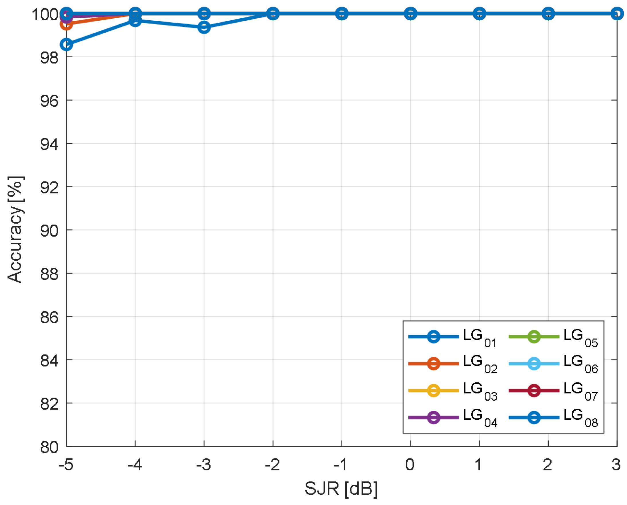
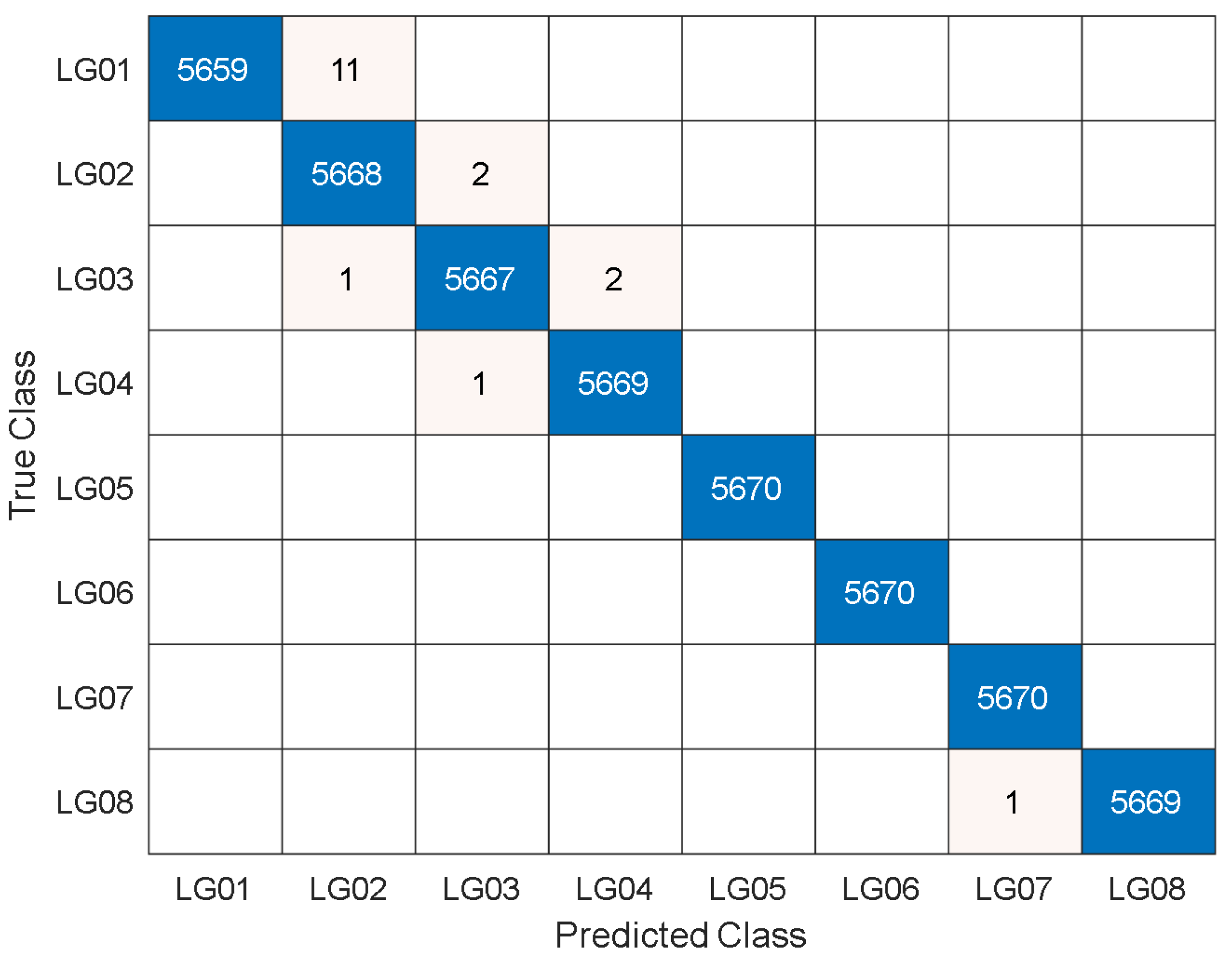
Classification of modes is performed using SVM; a machine learning algorithm that is widely used in modern applications to solve both classification and regression problems [28]. It has shown excellent performance in many disciplines such as medicine, engineering, finance, agriculture, etc. [29,30,31,32]. The main idea of an SVM is to utilize the data of two different classes to find a hyperplane that can separate the samples of these classes as much as possible.

For a given linearly separable set of data points $(x_i,y_i)$ with $i=1,2,\dots ,N,y_i\in \{-1,+1\}$, and $x_i\in R^2$, where N is the total number of data samples, the SVM seeks finding a linear hyperplane that separates the data samples of two classes. The linear hyperplane needs to satisfy the relation $w^{T}x+b=0$, where w and b are weights vector and bias of the hyperplane, with the following conditions:

$$\begin{gathered} w^{T}x+b\ge 1\mathrm{for}\mathrm{the}\mathrm{data}\mathrm{points}\mathrm{corresponding}\mathrm{to}{y}_i=+1, \\ {w}^{T}x+b\le -1\mathrm{for}\mathrm{the}\mathrm{data}\mathrm{points}\mathrm{corresponding}\mathrm{to}{y}_i=-1. \end{gathered}$$

The separating hyperplane is surrounded by two planes denoted by $w^{T}x+b=1$ and $w^{T}x+b=-1$, each of which has a distance from the separating plane called margin which is given by $2/\left|\right|w\left|\right|$ [26]. It is of importance to maximize the margin so that the SVM training process is optimized to find an optimal hyperplane that well separates the two classes as shown in Figure 7.

SVM can be used to classify nonlinearly separable data, after projecting it to higher dimensional space using a specific kernel. The role of kernel function is to transform the original data to another space, so that it facilitates the differentiation between data points of different classes. In addition to the linear function, various kernel functions like polynomial, sigmoid or radial basis functions can be used for classification purposes.

Although SVM was mainly introduced to solve binary classification problems, it is also developed to deal with multiclass classification problems. Two different methods are used to solve the multiclass classification problem, which is the “one-versus-one” and “one-versus-all” classification methods. In the “one-versus-one” method, multiple SVM models are constructed based on the number of classes, each of which is applied to classify two classes and the final decision is based on the majority vote. The resulting number of models is proportional to the number of classes M, which is given by $M(M-1)/2$. While in the “one-versus-all” method, the number of constructed models is equal to the number of classes. Each model is designed to classify between one class from one side and the rest of other classes from the other side, and the final decision of these models are based on majority vote [33,34,35].

3.3. Results

In the beginning, HOG features of all images are extracted following the previously described preprocessing steps. Then, the HOG dataset is divided into 70% for training and 30% for testing; a widely used division in literature [13,36,37]. One-versus-one multiclass SVM is constructed for the sake of classification tasks. The SVM classifier is built using error-correcting output codes (ECOC) algorithm to handle the multiclass classification problem [38]. ECOC algorithm is used to break down the classification problem into a set of binary classification problems when there are more than two classes. The SVM classifier is trained using a polynomial kernel of order two. Once the training phase is completed, the yielding model is evaluated using the testing set. To ensure the robustness of the proposed method, the process of training and testing is repeated ten times with random selection of training and testing sets. Figure 8 illustrates the block diagram of preprocessing steps and classification operation. The datasets of LG and Mux-LG are of size 15,120 images each, with eight different light modes, while the dataset of HG is of size 30,240 images generated using sixteen light modes.

Figure 9 depicts the accuracy achieved by the proposed method for the sake of classifying LG modes under jamming effect with SJR ranging from −5 dB to 3 dB. The figure clearly shows that the trained model is performing extremely well at higher SJR values; it reaches an accuracy of 100% at SJR = −2 dB or higher and fluctuates between 98.9% and 100% for lower SJR values. Figure 10 shows the misclassified LG modes in the form of a confusion matrix, which is computed from the test dataset over ten independent runs. It is observed that LG01 and LG02 modes have the highest misclassification rate of 0.2% which can be neglected. This is intuitively not surprising due to the similarity of these adjacent modes at lower SJR ratios. On the other hand, the proposed algorithm reached the optimum in regard to Mux-LG and HG modes classification. It achieved a classification accuracy of 100% over the SJR range of interest for both Mux-LG and HG modes.

It is worth noting that the proposed classification method outperforms the classification method reported in [14], which used the CNN classifier. While both methods achieved perfect results at higher SJR values, the proposed classification method does much better at lower SJR. For example, for LG modes classification, the proposed method achieved an accuracy of 98.9% at −5 dB while the method of [14] achieved 90.4% at the same value of SJR, as illustrated in Figure 11. The effectiveness of the proposed classification method over the CNN-based classification method is further demonstrated in Figure 12 and Figure 13 when Mux-LG and HG modes are considered.

4. SJR Estimation

Jamming causes a major problem in optical communications, as it can completely destroy the communication system. Therefore, it is of importance to estimate the SJR values for the sake of maintaining reliable communication. In this section, the estimation of the SJR value is investigated.

4.1. Algorithm Development

In our development, the raw images are first converted to grayscale images. Then, each image is resized to 100 × 100 pixels to reduce the computational cost. Further, each image is offset by subtracting its mean and normalized by its standard deviation. The zero-mean and normalized image is converted to a vector of size 100 samples, obtained by summing up the pixels’ values over the vertical axis. Figure 14 shows an example to illustrate the concept of projecting an image over its vertical axis. The resulting vector is rescaled to be within the range of −1 to 1 for further processing by an ANN.

The proposed ANN consists of an input layer, one hidden layer of size 20 neurons chosen empirically, and an output layer. The model makes use of a hyperbolic tangent sigmoid transfer function at the hidden layer and a linear transfer function at the output layer. The Levenberg-Marquardt algorithm has been used to adjust the model’s weights. The network was trained using 70% of data samples, while the rest were used for the testing phase. Figure 15 shows the block diagram of the proposed algorithm for SJR estimation.

4.2. Results

The experimental results presented here consider SJR values ranging between −5 dB and 3 dB. The estimation is performed using LG, Mux-LG, and HG modes over fifty independent runs to show the robustness of the proposed method. Figure 16 depicts the MSE of predicting the value of SJR per each run when LG, Mux-LG, and HG modes are employed. Based on the results of Figure 16, the proposed algorithm achieves average MSEs of 0.167, 0.155, and 0.172 dB at the testing phase to predict the SJR in the case of LG, Mux-LG, and HG transmissions, respectively. Also, Figure 17 illustrates the mean and standard deviation (STD) of predicted SJR values over fifty independent runs for the modes under consideration.

5. Discussion

CIn this work, we addressed two ML applications in data transmission using structured light beams for FSO systems under the jamming effect. First, we proposed HOG and SVM-based algorithms to identify structured light modes under the jamming effect. The experimentally generated light beams form three coding schemes which were based on LG, Mux-LG, and HG shape structures. In particular, the proposed algorithm achieved a classification accuracy of 98.9% at SJR less than −2 dB and 100% at higher SJR values when LG modes are employed. Moreover, the proposed classification algorithm achieved an accuracy of 100% for Mux-LG and HG modes under SJR values between −5 dB and 3 dB. The proposed classification algorithm has shown superior performance to identify the jammed structured light beam. These outstanding results are intuitively not surprising because the ML algorithm utilized for classifications has been preceded by proper preprocessing steps applied to the input data (modes). Specifically, the preprocessing steps have played a great role to reduce background noise, improve contrast through image equalization, and extract features using an elegant algorithm based on HOG. Second, the results presented in Section 4.2 have shown that the vector resulting from the projection of a received jammed mode onto its image’s vertical axis is sufficient to capture the level of jamming energy. This is evident from the results of the proposed algorithm where it achieved average MSEs of 0.167, 0.155, and 0.172 dB computed over fifty independent runs to predict the SJR value in the case of LG, Mux-LG, and HG transmissions, respectively.

6. Conclusions

In this study, we proposed two classification and estimation algorithms considering jamming when a structured light beam is transmitted over a free-space optical communication link. Our development was based on experimental data consisting of different modes of a structured light beam which include the 8-ary LG, 8-ary superposition-LG, and 16-ary HG formats. First, we utilized the algorithms of the support vector machine and histogram of oriented gradients for the sake of light beam modes classification. Second, we proposed a simple ANN-based model to estimate the SJR values. From the results presented in this work, we can conclude that preprocessing of input modes images considerably enhances the capability of ML-based structured light identification algorithms. Furthermore, the use of ML algorithms provides great effectiveness not only in identifying structured light modes but also in estimating the signal-to-interference ratio in a harsh jamming environment.

References

1. Malik, A.; Singh, P. Free space optics: Current applications and future challenges. Int. J. Opt. 2015, 2015, 945483. [Google Scholar] [CrossRef] [Green Version]
2. Trichili, A.; Park, K.; Zghal, M.; Ooi, B.S.; Alouini, M. Communicating Using Spatial Mode Multiplexing: Potentials, Challenges, and Perspectives. IEEE Commun. Surv. Tutor. 2019, 21, 3175–3203. [Google Scholar] [CrossRef] [Green Version]
3. Vigneshwaran, S.; Muthumani, I.; Raja, A.S. Investigations on free space optics communication system. In Proceedings of the 2013 International Conference on Information Communication and Embedded Systems (ICICES), Chennai, India, 21–22 February 2013; pp. 819–824. [Google Scholar]
4. Singh, J.; Kumar, N. Performance analysis of different modulation format on free space optical communication system. Optik 2013, 124, 4651–4654. [Google Scholar] [CrossRef]
5. Ren, Y.; Xie, G.; Huang, H.; Ahmed, N.; Yan, Y.; Li, L.; Bao, C.; Lavery, M.P.; Tur, M.; Neifeld, M.A.; et al. Adaptive-optics-based simultaneous pre-and post-turbulence compensation of multiple orbital-angular-momentum beams in a bidirectional free-space optical link. Optica 2014, 1, 376–382. [Google Scholar] [CrossRef]
6. Huang, H.; Xie, G.; Ren, Y.; Yan, Y.; Bao, C.; Ahmed, N.; Ziyadi, M.; Chitgarha, M.; Neifeld, M.; Dolinar, S.; et al. 4 × 4 MIMO equalization to mitigate crosstalk degradation in a four-channel free-space orbital-angular-momentum-multiplexed system using heterodyne detection. In Proceedings of the IET 39th European Conference and Exhibition on Optical Communication (ECOC 2013), London, UK, 22–26 September 2013; pp. 1–3. [Google Scholar]
7. Huang, H.; Cao, Y.; Xie, G.; Ren, Y.; Yan, Y.; Bao, C.; Ahmed, N.; Neifeld, M.A.; Dolinar, S.J.; Willner, A.E. Crosstalk mitigation in a free-space orbital angular momentum multiplexed communication link using 4 × 4 MIMO equalization. Opt. Lett. 2014, 39, 4360–4363. [Google Scholar] [CrossRef] [PubMed]
8. Krenn, M.; Fickler, R.; Fink, M.; Handsteiner, J.; Malik, M.; Scheidl, T.; Ursin, R.; Zeilinger, A. Communication with spatially modulated light through turbulent air across Vienna. New J. Phys. 2014, 16, 113028. [Google Scholar] [CrossRef]
9. Wang, Z.; Dedo, M.I.; Guo, K.; Zhou, K.; Shen, F.; Sun, Y.; Liu, S.; Guo, Z. Efficient recognition of the propagated orbital angular momentum modes in turbulences with the convolutional neural network. IEEE Photonics J. 2019, 11, 1–14. [Google Scholar] [CrossRef]
10. Rostami, S.; Saad, W.; Hong, C.S. Deep learning with persistent homology for orbital angular momentum (OAM) decoding. IEEE Commun. Lett. 2019, 24, 117–121. [Google Scholar] [CrossRef] [Green Version]
11. Freitas, B.S.; Runge, C.J.; Portugheis, J.; de Oliveira, I.; Dias, U. Optimized OAM Laguerre-Gauss Alphabets for Demodulation using Machine Learning. In Proceedings of the IEEE 2020 IEEE 8th International Conference on Photonics (ICP), Kota Bharu, Malaysia, 12 May–30 June 2020; pp. 24–25. [Google Scholar]
12. Li, J.; Zhang, M.; Wang, D.; Wu, S.; Zhan, Y. Joint atmospheric turbulence detection and adaptive demodulation technique using the CNN for the OAM-FSO communication. Opt. Express 2018, 26, 10494–10508. [Google Scholar] [CrossRef]
13. Ragheb, A.; Saif, W.; Trichili, A.; Ashry, I.; Esmail, M.A.; Altamimi, M.; Almaiman, A.; Altubaishi, E.; Ooi, B.S.; Alouini, M.S.; et al. Identifying structured light modes in a desert environment using machine learning algorithms. Opt. Express 2020, 28, 9753–9763. [Google Scholar] [CrossRef] [PubMed] [Green Version]
14. Ragheb, A.M.; Saif, W.S.; Alshebeili, S.A. ML-Based Identification of Structured Light Schemes under Free Space Jamming Threats for Secure FSO-Based Applications. Photonics 2021, 8, 129. [Google Scholar] [CrossRef]
15. El-Meadawy, S.A.; Shalaby, H.M.; Ismail, N.A.; Abd El-Samie, F.E.; Farghal, A.E. Free-space 16-ary orbital angular momentum coded optical communication system based on chaotic interleaving and convolutional neural networks. Appl. Opt. 2020, 59, 6966–6976. [Google Scholar] [CrossRef] [PubMed]
16. Trichili, A.; Issaid, C.B.; Ooi, B.S.; Alouini, M.S. A CNN-based structured light communication scheme for internet of underwater things applications. IEEE Internet Things J. 2020, 7, 10038–10047. [Google Scholar] [CrossRef] [Green Version]
17. Siegman, A.E. Lasers; University Science Books: Mill Valley, CA, USA, 1986. [Google Scholar]
18. Luan, H.; Lin, D.; Li, K.; Meng, W.; Gu, M.; Fang, X. 768-ary Laguerre-Gaussian-mode shift keying free-space optical communication based on convolutional neural networks. Opt. Express 2021, 29, 19807–19818. [Google Scholar] [CrossRef] [PubMed]
19. Dhal, K.G.; Das, A.; Ray, S.; Gálvez, J.; Das, S. Histogram equalization variants as optimization problems: A review. Arch. Comput. Methods Eng. 2021, 28, 1471–1496. [Google Scholar] [CrossRef]
20. Gonzalez, R.C. Digital Image Processing, 4th ed.; Pearson education India: Chennai, India, 2017. [Google Scholar]
21. Ma, J.; Jiang, X.; Fan, A.; Jiang, J.; Yan, J. Image matching from handcrafted to deep features: A survey. Int. J. Comput. Vis. 2021, 129, 23–79. [Google Scholar] [CrossRef]
22. Wang, Y.; Zhu, X.; Wu, B. Automatic detection of individual oil palm trees from UAV images using HOG features and an SVM classifier. Int. J. Remote Sens. 2019, 40, 7356–7370. [Google Scholar] [CrossRef]
23. Seemanthini, K.; Manjunath, S. Human detection and tracking using HOG for action recognition. Procedia Comput. Sci. 2018, 132, 1317–1326. [Google Scholar]
24. Ouerhani, Y.; Alfalou, A.; Brosseau, C. Road mark recognition using HOG-SVM and correlation. In Proceedings of the Optics and Photonics for Information Processing XI, San Diego, CA, USA, 7–8 August 2017; Volume 10395, pp. 119–126. [Google Scholar]
25. Altowaijri, A.H.; Alfaifi, M.S.; Alshawi, T.A.; Ibrahim, A.B.; Alshebeili, S.A. A Privacy-Preserving Iot-Based Fire Detector. IEEE Access 2021, 9, 51393–51402. [Google Scholar] [CrossRef]
26. Firuzi, K.; Vakilian, M.; Phung, B.T.; Blackburn, T.R. Partial discharges pattern recognition of transformer defect model by LBP & HOG features. IEEE Trans. Power Deliv. 2018, 34, 542–550. [Google Scholar]
27. Dalal, N.; Triggs, B. Histograms of oriented gradients for human detection. In Proceedings of the IEEE 2005 IEEE Computer Society Conference on Computer Vision and Pattern Recognition (CVPR’05), San Diego, CA, USA, 20–25 June 2005; Volume 1, pp. 886–893. [Google Scholar]
28. Zhou, Z.H. Support vector machine. In Machine Learning; Springer: New York, NY, USA, 2021; pp. 129–153. [Google Scholar]
29. Battineni, G.; Chintalapudi, N.; Amenta, F. Machine learning in medicine: Performance calculation of dementia prediction by support vector machines (SVM). Inform. Med. Unlocked 2019, 16, 100200. [Google Scholar] [CrossRef]
30. Zendehboudi, A.; Baseer, M.A.; Saidur, R. Application of support vector machine models for forecasting solar and wind energy resources: A review. J. Clean. Prod. 2018, 199, 272–285. [Google Scholar] [CrossRef]
31. Yang, R.; Yu, L.; Zhao, Y.; Yu, H.; Xu, G.; Wu, Y.; Liu, Z. Big data analytics for financial Market volatility forecast based on support vector machine. Int. J. Inf. Manag. 2020, 50, 452–462. [Google Scholar] [CrossRef]
32. Chen, Y.; Wu, Z.; Zhao, B.; Fan, C.; Shi, S. Weed and corn seedling detection in field based on multi feature fusion and support vector machine. Sensors 2021, 21, 212. [Google Scholar] [CrossRef] [PubMed]
33. Saif, W.S.; Esmail, M.A.; Ragheb, A.M.; Alshawi, T.A.; Alshebeili, S.A. Machine learning techniques for optical performance monitoring and modulation format identification: A survey. IEEE Commun. Surv. Tutor. 2020, 22, 2839–2882. [Google Scholar] [CrossRef]
34. Bhavsar, H.; Panchal, M.H. A review on support vector machine for data classification. Int. J. Adv. Res. Comput. Eng. Technol. (IJARCET) 2012, 1, 185–189. [Google Scholar]
35. Mayoraz, E.; Alpaydin, E. Support vector machines for multi-class classification. In International Work-Conference on Artificial Neural Networks; Springer: New York, NY, USA, 1999; pp. 833–842. [Google Scholar]
36. Esmail, M.A.; Saif, W.S.; Ragheb, A.M.; Alshebeili, S.A. Free space optic channel monitoring using machine learning. Opt. Express 2021, 29, 10967–10981. [Google Scholar] [CrossRef] [PubMed]
37. Wang, C.; Fu, S.; Wu, H.; Luo, M.; Li, X.; Tang, M.; Liu, D. Joint OSNR and CD monitoring in digital coherent receiver using long short-term memory neural network. Opt. Express 2019, 27, 6936–6945. [Google Scholar] [CrossRef]
38. Dietterich, T.G.; Bakiri, G. Solving multiclass learning problems via error-correcting output codes. J. Artif. Intell. Res. 1994, 2, 263–286. [Google Scholar] [CrossRef] [Green Version]
Figure 1. Experimentally generated beam profiles of: (a) LG, (b) Mux-LG, and (c) HG modes with no jamming interference. Reprinted from ref. [14].
Photonics 09 00200 g001
Figure 2. Measured beam profiles under jamming effect at SJRs of: (a) −5 dB, (b) 0 dB, and (c) 3 dB. Reprinted from ref. [14].
Photonics 09 00200 g002
Figure 3. Conceptual block diagram of experimental setup. LD: laser diode, POL: polarizer, HWP: half-wave plate, CCD: charge-coupled device, and SLM: spatial light modulator.
Photonics 09 00200 g003
Figure 4. (a) Original histogram of grayscale image, (b) Histogram with background set to 0, and (c) Equalized histogram.
Photonics 09 00200 g004
Figure 5. (a) Original image, (b) Grayscale image, (c) Grayscale image with background set to 0, and (d) Image after histogram equalization.
Photonics 09 00200 g005
Figure 6. (a) HOG of an LG08 mode, (b) HOG of an Mux-LG0±8 mode, (c) HOG of an HG33 mode.
Photonics 09 00200 g006
Figure 7. Illustration of binary SVM classifier.
Photonics 09 00200 g007
Figure 8. Block diagram of the proposed algorithm for light beam mode classification.
Photonics 09 00200 g008
Figure 9. Accuracy of LG modes classification.
Photonics 09 00200 g009
Figure 10. Confusion matrix of LG modes classification.
Photonics 09 00200 g010
Figure 11. Results of the proposed SVM-Based and CNN-based classification methods when LG modes are considered.
Photonics 09 00200 g011
Figure 12. Results of the proposed SVM-Based and CNN-based classification methods when Mux-LG modes are considered.
Photonics 09 00200 g012
Figure 13. Results of the proposed SVM-Based and CNN-based classification methods when HG modes are considered.
Photonics 09 00200 g013
Figure 14. (a) Matrix showing the pixels of an 5 × 5 image, (b) The vector resulting from projecting the matrix over its vertical axis.
Photonics 09 00200 g014
Figure 15. Block diagram of SJR estimation algorithm.
Photonics 09 00200 g015
Figure 16. MSE of estimating the SJR over fifty independent runs for: LG, Mux-LG, and HG transmissions.
Photonics 09 00200 g016
Figure 17. Mean ± STD of estimated SJR values over fifty independent runs for: (a) LG, (b) Mux-LG, and (c) HG transmissions.
Photonics 09 00200 g017
Publisher’s Note: MDPI stays neutral with regard to jurisdictional claims in published maps and institutional affiliations.