Article

A Method of Range Walk Error Correction in SiPM LiDAR with Photon Threshold Detection

1
School of Information Science and Engineering, Fudan University, 220 Handan Road, Shanghai 200433, China
2
Academy for Engineering and Technology, Fudan University, 220 Handan Road, Shanghai 200433, China
*
Author to whom correspondence should be addressed.
Photonics 2022, 9(1), 24; https://doi.org/10.3390/photonics9010024
Submission received: 17 November 2021 / Revised: 21 December 2021 / Accepted: 23 December 2021 / Published: 1 January 2022
(This article belongs to the Special Issue Optical Sensing)

Abstract

:
A silicon photomultiplier (SiPM) LiDAR with photon threshold detection can achieve high dynamic performance. However, the number fluctuations of echo signal photons lead to the range walk error (RWE) in SiPM LIDARs. This paper derives the RWE model of SiPM LiDAR by using the LiDAR equation and statistical property of SiPM’s response. Based on the LiDAR system parameters and the echo signal intensity, which is obtained through the SiPM’s photon-number-resolving capability, the RWE is calculated through the proposed model. After that, we carry out experiments to verify its effectiveness. The result shows that the method reduces the RWE in TOF measurements using photon threshold detection from 36.57 cm to the mean deviation of 1.95 cm, with the number of detected photons fluctuating from 1.3 to 46.5.

1. Introduction

A single-photon avalanche diode (SPAD) has been widely used in remote laser ranging systems due to its single-photon detection sensitivity and high time resolution [1,2,3]. SPAD functions as a binary device with a deadtime [4]. The time-to-digital converter (TDC) for TOF computation can only timestamp the first detected photon in a SPAD pixel. Therefore, a SPAD LiDAR system encounters the problem of a high false alarm rate, which becomes prominent when the background light is strong. To solve this problem, References [5,6,7] utilize the time-correlated single-photon counting (TCSPC) technique to calculate the flight time by counting the trigger time distribution. However, TCSPC requires thousands of successive measurements to improve the signal-to-noise ratio (SNR) and calculate the time of flight (TOF). The long acquisition time restricts the application of SPAD LiDAR in areas such as autonomous driving, given the requirements for high frame rate imaging and fast-moving target tracking [8].
SiPMs are large photosensitive area detectors that consist of parallel SPAD pixels, and each pixel has an independent quenching circuit [9]. In analog SiPM, the summation of each pixel’s response constitutes the analog output signal of SiPM [10,11,12]. As a result, the signal of SiPM is proportional to the number of incident photons. In digital SiPM, the SPAD frontend is an active circuit that sets a fixed and well-defined deadtime after each ignition and provides a digital pulse when a photon is detected. The output of all microcells is combined through logic gates. The digital output is directly the number of fired cells [11,12]. Regarding SiPM’s photon-number-resolving capability, compared to SPAD LiDAR, SiPM LiDAR can utilize the photon threshold to filter out low photon numbers. The threshold can lower the false alarm rate and improve the SNR of the LiDAR system [13]. In addition to this, setting the photon threshold helps suppress the ranging uncertainty caused by the pulse width of the laser. These advantages help the SiPM LiDAR system achieve a better dynamic range.
For wide-dynamic-range applications, SiPM LiDAR requires high accuracy when measuring targets with extreme variations in reflectivity and angles. Moreover, the RWE caused by the number fluctuation of the received photons is the dominating influential factor for accurate ranging. References [14,15,16,17] establish several methods to reduce RWE emerging in SPAD LiDAR systems. Reference [18] proposes a correction method for RWE in LiDAR with a photomultiplier tube. References [19,20,21] discuss the accuracy of linear APD LiDAR using a fixed threshold discriminator, the constant fraction discriminator (CFD) method and the peak detection method (PKD). However, to date, there have been few related studies focusing on the RWE reduction in SiPM LiDAR with threshold detection.
In this article, an RWE correction method of an SiPM LiDAR system with threshold detection is proposed. First, we establish a theoretical RWE model containing the response characteristics of SiPM and the photon threshold method. Thereafter, the RWE is calculated through the above model. In the proposed RWE model using the photon threshold method, we derive the relationship between RWE and the number of detected photons, which can be obtained via either analog SiPM or digital SiPM. Therefore, the proposed method is available in the two types of SiPM LiDAR systems. Groups of experiments with different echo light intensities are performed to measure the distance to a fixed target. In each group, we conduct the correction method to offset the RWE emerging in the result of the fixed photon threshold detection. Meanwhile, the CFD and PKD methods are utilized for comparison with the proposed method. Finally, we develop a method that utilizes the detection probability of the photon threshold detection to estimate the mean number of detected photons instead of using the signal of SiPM, which may simplify the system. As proved by the experiments, this method can work at the few-photon level.

2. Theoretical Analysis

2.1. Laser Propagation Equation

The D-TOF LiDAR system delivers a narrow-width laser pulse to the target. The power of an emitted Gaussian pulse [22] can be described with the average single-pulse energy ET as follows:
P E m i t ( t ) = E T 1 2 π σ f e t 2 2 σ f 2
where PEmit(t) is the power of the emitted pulse, and σf is the emitted pulse width. When the pulse is scattered from a Lambertian target at distance R, the received number of photons, NPhoton(t), can be derived from Equation (1) [16] as
N P h o t o n ( t ) = N S 1 2 π σ S e t 2 2 σ S 2 + N N o i s e
where NNoise is the background noise rate, and σS is the received pulse width. We assume σ S σ f in this manuscript because the transmitted pulse width is in the order of nanoseconds [23]; NS is the mean number of received signal photons, which can be calculated as [24]
N S = E T η T η R η A 2 ρ A R π R 2 h v
where η T is the transmission of the transmitter; η R is the transmission of the receiver optic; η A is the one-way transmission of the atmosphere; ρ is the reflectivity of the target; A R is the area of the aperture of the receiver; h is the Plank constant; and v is the frequency of the laser.

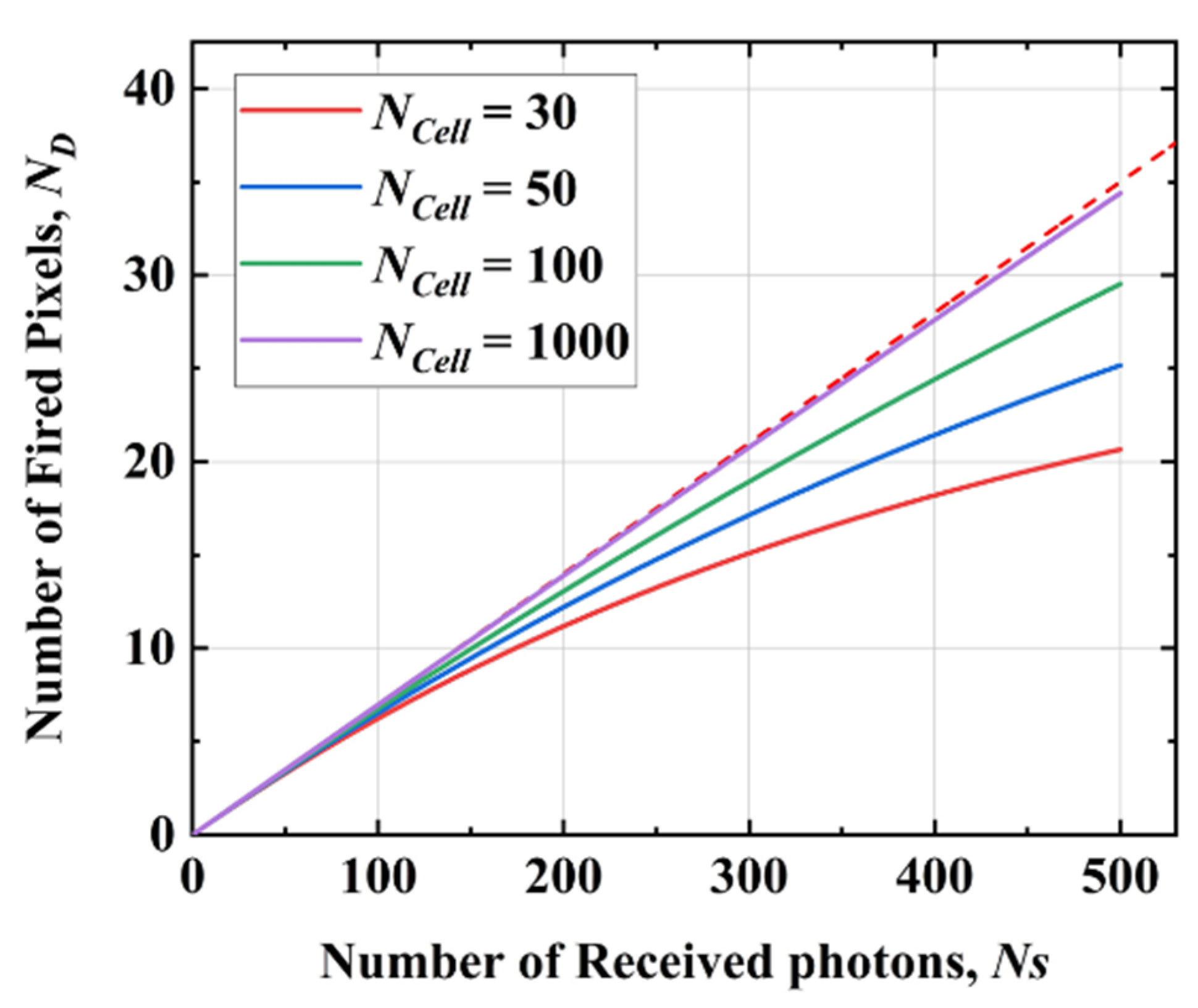
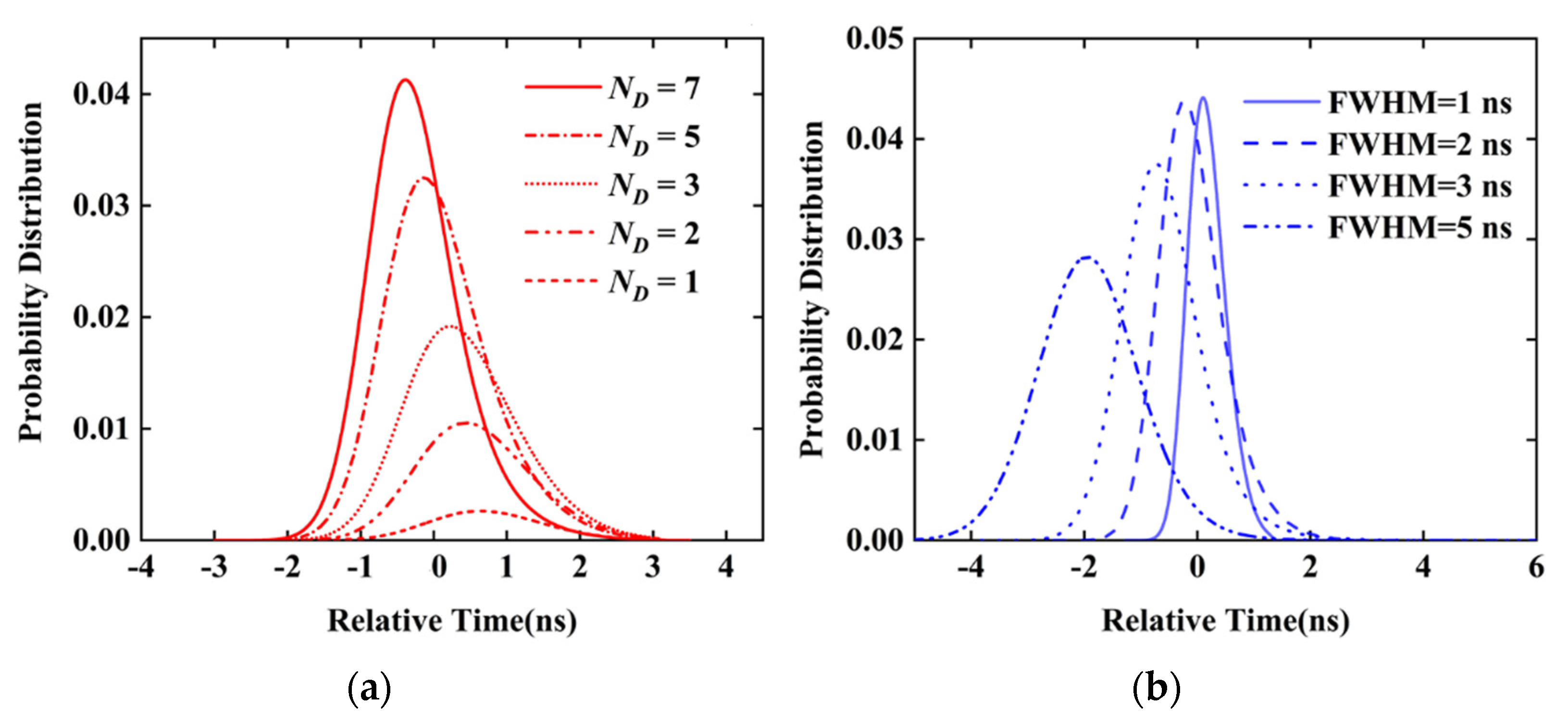
2.2. SiPM Response Model

Assuming that the number of arriving photons on each pixel is evenly distributed, then, in any time interval ( t 1 , t 2 ) , the mean number of photons hitting each pixel, N ¯ , can be derived from Equation (2) as
N ¯ ( t 1 , t 2 ) = t 1 t 2 N P h o t o n ( t ) d t N C e l l
where NCell is the number of pixels in SiPM. Poisson distribution is an appropriate model to describe the response of a pixel [25]. The probability that a pixel responds in the ith time bin is derived from Equation (4) [26]:
P D _ b i n ( i 1 , i ) = 1 e N ¯ ( τ b i n ( i 1 ) , τ b i n i ) η q
where ηq is the photon detection efficiency of SiPM; i is an integer larger than 0; and τbin is the length of a time bin, which corresponds to the timing resolution of the TDC. Therefore, the mean number of fired pixels in one measurement, ND, can be calculated as
N D = N C e l l ( 1 e ( N T o t a l η q N C e l l ) )
here,
N T o t a l = 0.5 T S i g n a l 0.5 T S i g n a l N P h o t o n ( t ) d t = N S + N N o i s e T S i g n a l
Therefore, NS can also be calculated through Equations (6) and (7) as
N S = N C e l l η q ln ( N C e l l N C e l l N D ) N N o i s e T S i g n a l
where NTotal is the number of arrived photons (including ambient noise) in a signal duration. TSignal is the effective signal duration, usually TSignal > 6σS. As seen in Equation (3), environment parameters, such as the one-way transmission of the atmosphere and the reflectivity of the target, are needed to calculate Ns. However, according to Equation (8), we can estimate NS by the number of fired pixels, which can be obtained from the signal of SiPM. ND has a linear relation with Ns when NCell >> ND as seen in Figure 1.
Considering that the response of each pixel is independent and that the probability of k pixel responses in a time interval PCell obeys the binomial distribution [25], then the probability is derived from Equation (5) as
P C e l l ( ( i 1 , i ) , k ) = ( N C e l l k ) P D _ b i n k ( i 1 , i ) ( 1 P D _ b i n ( i 1 , i ) ) N C e l l k
In fact, if more than one photon hits a pixel, only one can be detected, which causes non-linear loss. In Equation (9), the nonlinear loss is not considered, because we limited our signal to a few photons where nonlinear loss has a low effect on the results [13]. This is due to the relatively low photon number compared to the number of pixels, which is about two orders of magnitude less in the experiment.
For light detection at the few-photon level, the number of fired pixels is very small compared to thousands or even tens of thousands of pixels in the SiPM. Meanwhile, the probability of detecting a photon in a single pixel is minimal; therefore, Equation (9) can be approximated as a Poisson distribution [27]:
P C e l l ( ( i 1 , i ) , k ) = ( N C e l l P D _ b i n ( i 1 , i ) ) k e N C e l l P D _ b i n ( i 1 , i ) k !
In the fixed threshold detection method for APD LiDAR, the arrival time of the light is determined when the voltage of the detector reaches a given voltage amplitude. The method for the SiPM LiDAR is similar. After the light is detected by SiPM, the photon number is then thresholded by a one-bit comparator, which stops the timer when the voltage of SiPM, caused by the detection of the arriving photons, exceeds the given threshold. The threshold detection probability in the ith time bin P(i) is calculated by summing the probability of all possible events that the accumulative number of fired pixels exceeds as the threshold photon number k in the ith time bin. Therefore, P(i) can be derived from Equation (10) as
P ( i ) = u = 0 k 1 ( P C e l l ( ( 0 , i 1 ) , u ) ( 1 v = 0 k u 1 P C e l l ( ( i 1 , i ) , v ) ) )
where u is the number of fired pixels before the ith time bin, and v is the fired pixels within the ith time bin. The event where the accumulative number of fired pixels exceeds k in the ith time bin must satisfy that u + vk and v ≥ 1. Then, the whole detection probability PD of one shot can be obtained from Equation (11) as
P D = s i g n a l b i n s P ( i )
where signalbins is a collection of intervals (−0.5TSignal, 0.5TSignal) divided into cells with a length of τbin.
Figure 2 is the simulation result based on Equation (11). The time bin is of the interval (−0.5TSignal, 0.5TSignal). The origin of the time axis is the center of the echo signal. The photon threshold k = 3. The σS is 1.02 ns, the number of pixels of SiPM is NCell = 2688, and the mean number of fired pixels is ND = 7, 5, 3, 2, 1. Figure 2a shows the detection probability based on Equation (11) under different echo light intensities. It indicates that, as the intensity of the echo decreases, the center of the detection probability distribution shifts to the right, and the full width at half maximum (FWHM) increases. Figure 2b shows the detection probability under different laser pulses (ND = 7, FWHM = 1, 2, 3, 5 ns). Figure 2b indicates that, as the FWHM increases, the probability distribution center shifts to the right, and the ranging uncertainty increases. The centroid algorithm can calculate the triggered time using the following equation:
T S i m = s i g n a l b i n s P ( i ) i τ b i n s i g n a l b i n s P ( i )
Therefore, the range walk error can be calculated using the following equation:
R W E = c 2 ( T S i m T R e f )
where TRef is the reference time of flight. In the following experiment, TSim (ND = 46.5) is recognized as TRef because the experimental ND varies from 1.3 to 46.5, and RWE is almost unchanged when ND becomes large. Figure 3 depicts the simulation between RWE, the detection probability and ND with a different photon threshold k. Figure 3a shows that the RWE is large when ND varies from 1 and 10, while the rate of change in RWE is small when ND becomes larger than 10. We also find that setting a higher threshold fails to improve measurement accuracy, although it may help reduce false alarms and improve system precision. In addition, as seen in Figure 3b, setting the photon threshold may lower the detection probability when few photons are received, as the threshold may filter out some signal photons, thus causing a loss in detection.

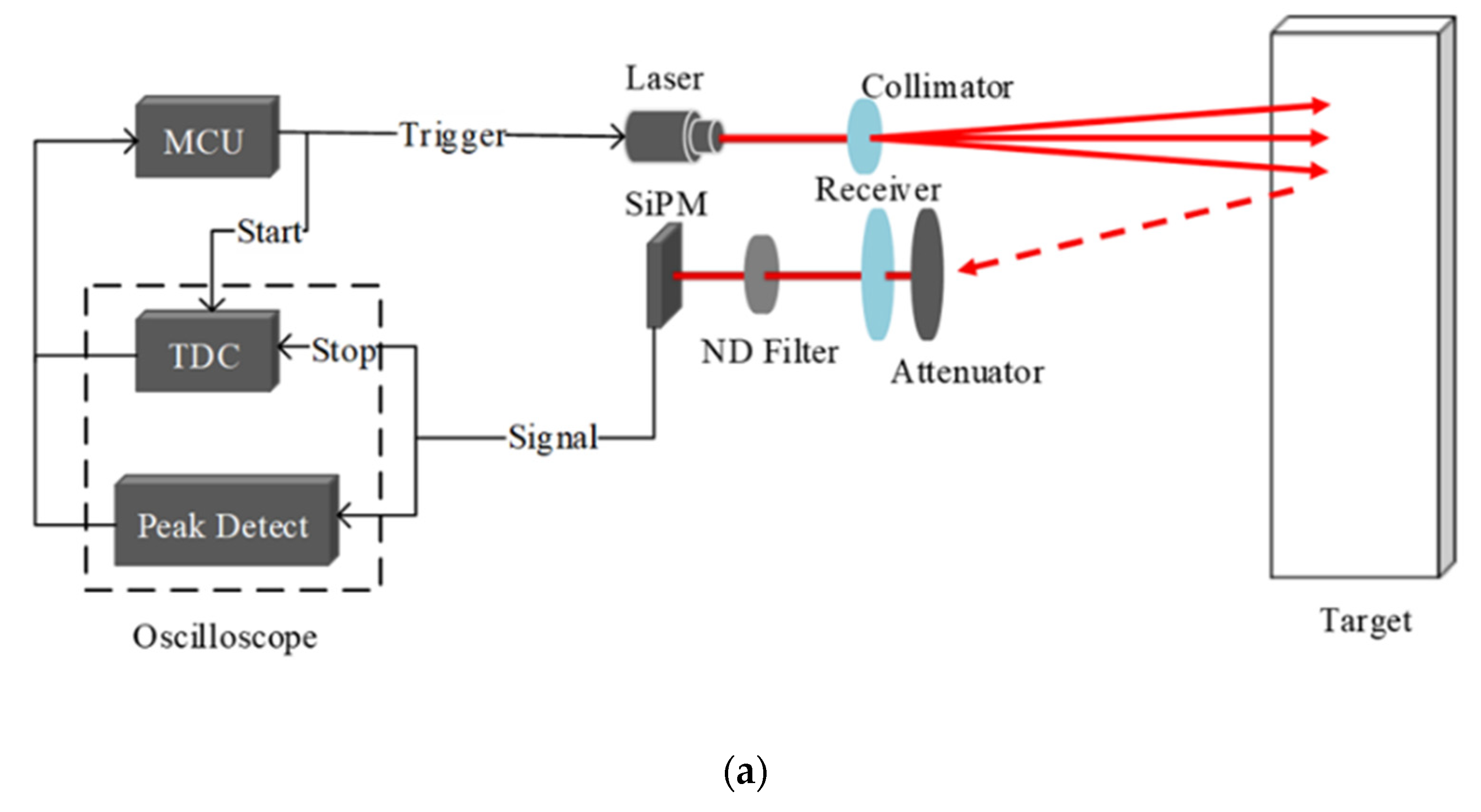
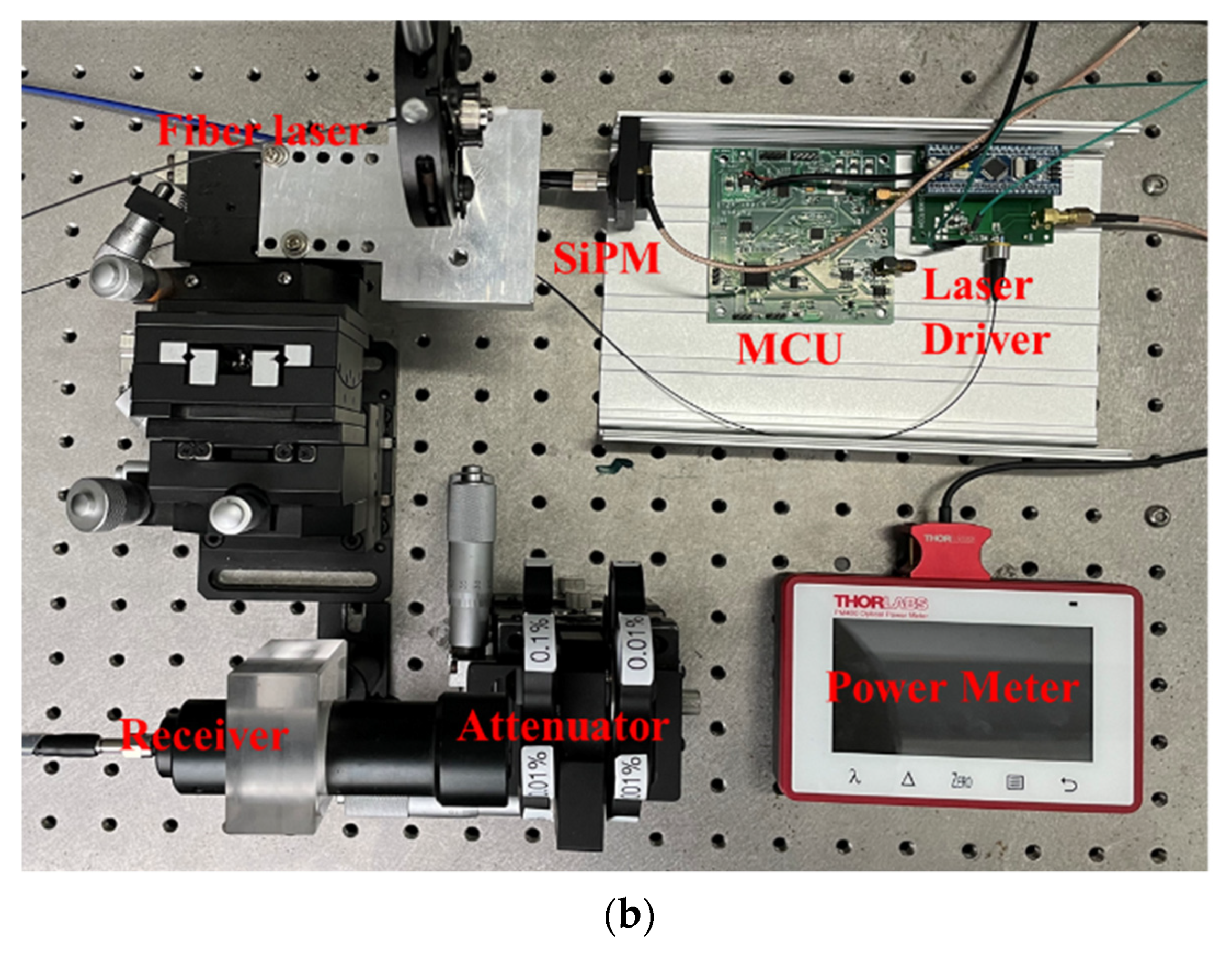
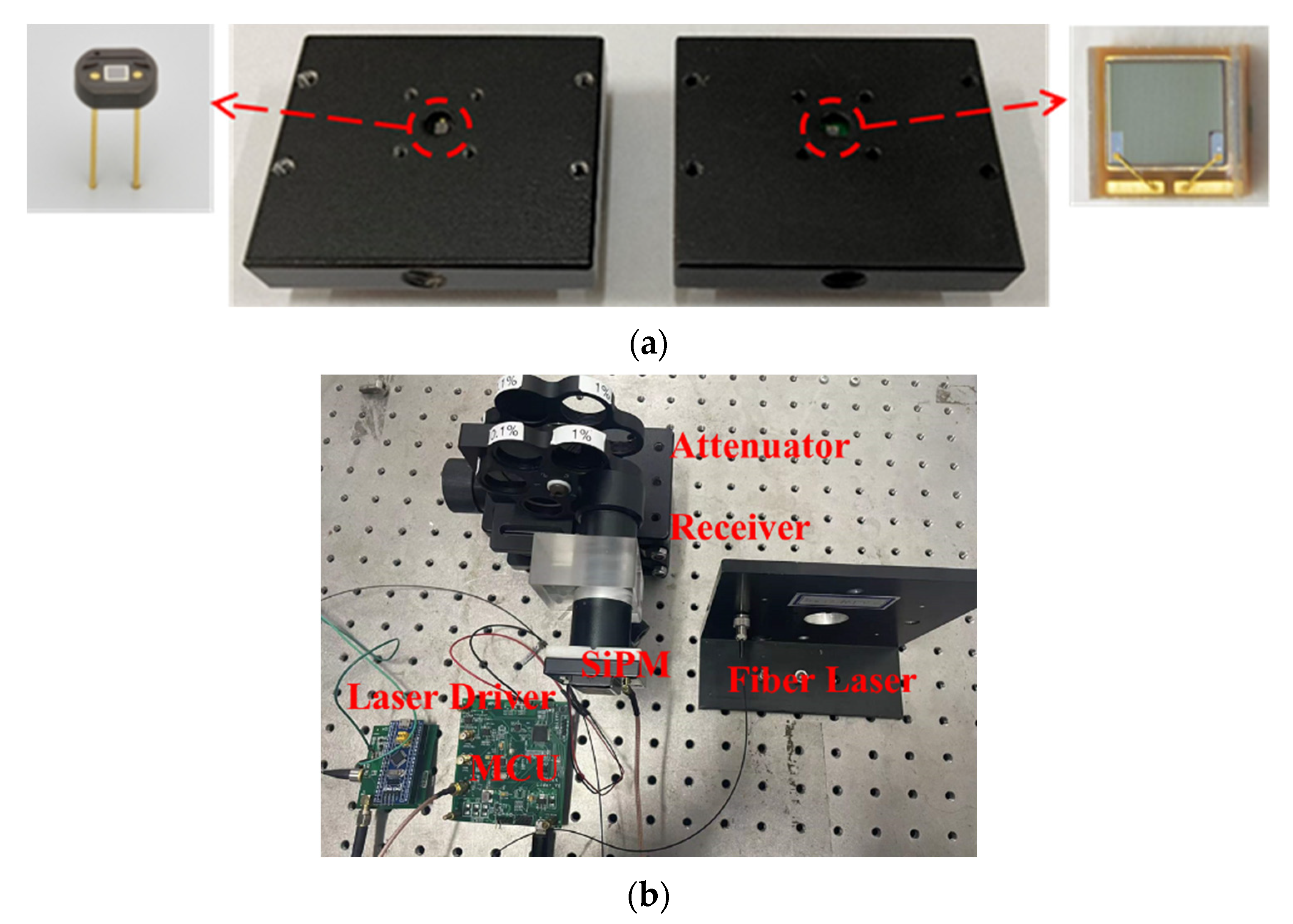
3. Experiments and Analysis

Figure 4 shows the system structure diagram and the experimental platform. The MCU generates the trigger signal divided into two channels. One channel triggers the laser driver to generate the pulsed laser, and the other one is transmitted to the oscilloscope. The emitted laser with a certain divergence angle is diffusely reflected by the flat target, and, finally, only the reflected light in a specific direction is received by the detector. Then, the SiPM signal is transmitted to the oscilloscope, and functions are utilized to measure the time interval between the trigger and the echo signal. A multimode semiconductor fiber laser (LSPLD905-50W) with a wavelength center of 905 nm is used as the light source. The FWHM of the laser pulse is 2.40 ns, and the peak power is adjustable within 50 W. The laser pulse emitted by the fiber passes through the collimating lens and is reflected by the target. Thereafter, it hits the detector through the attenuator, the receiving lens and the 905 nm narrowband filter. The analog SiPM detector used is the MPPC module (C14193-1325SA, Hamamatsu) with 2668 Si-APD pixel SiPM (S13720-1325CS, Hamamatsu) inside. The PDE (photon detection efficiency) of 7% is used for photons with a wavelength of 905 nm. The oscilloscope used is the Infinium (DSO90604A, Angilent) with a 6 GHz bandwidth and 20 GSa/s, which means that the time resolution is 50 ps. The power meter used is PM101 from Thorlabs.

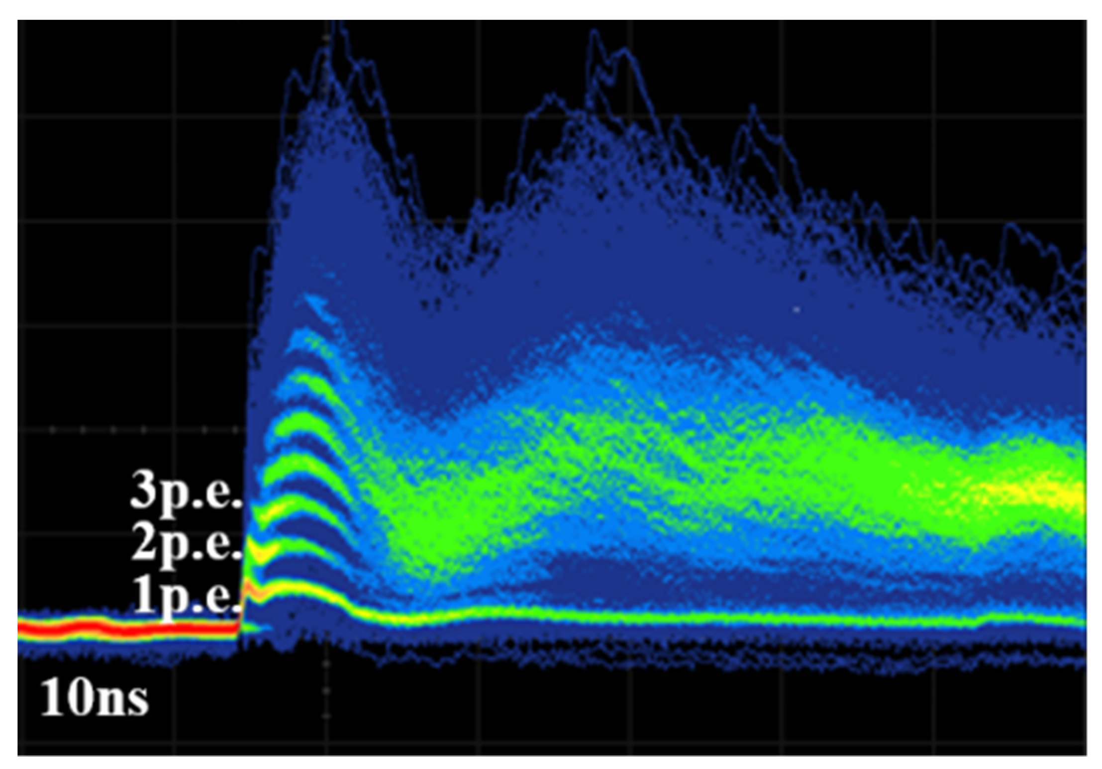
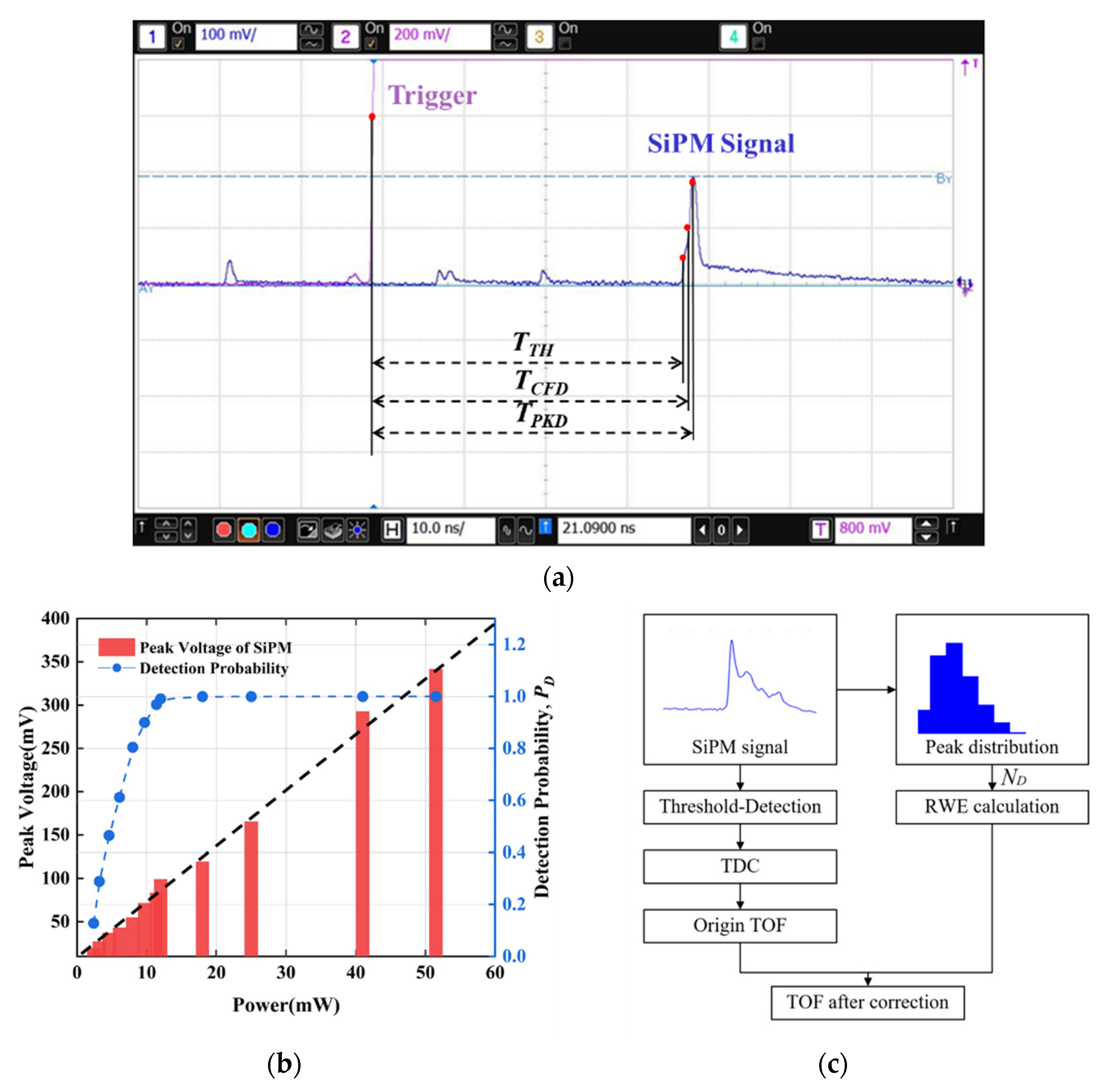
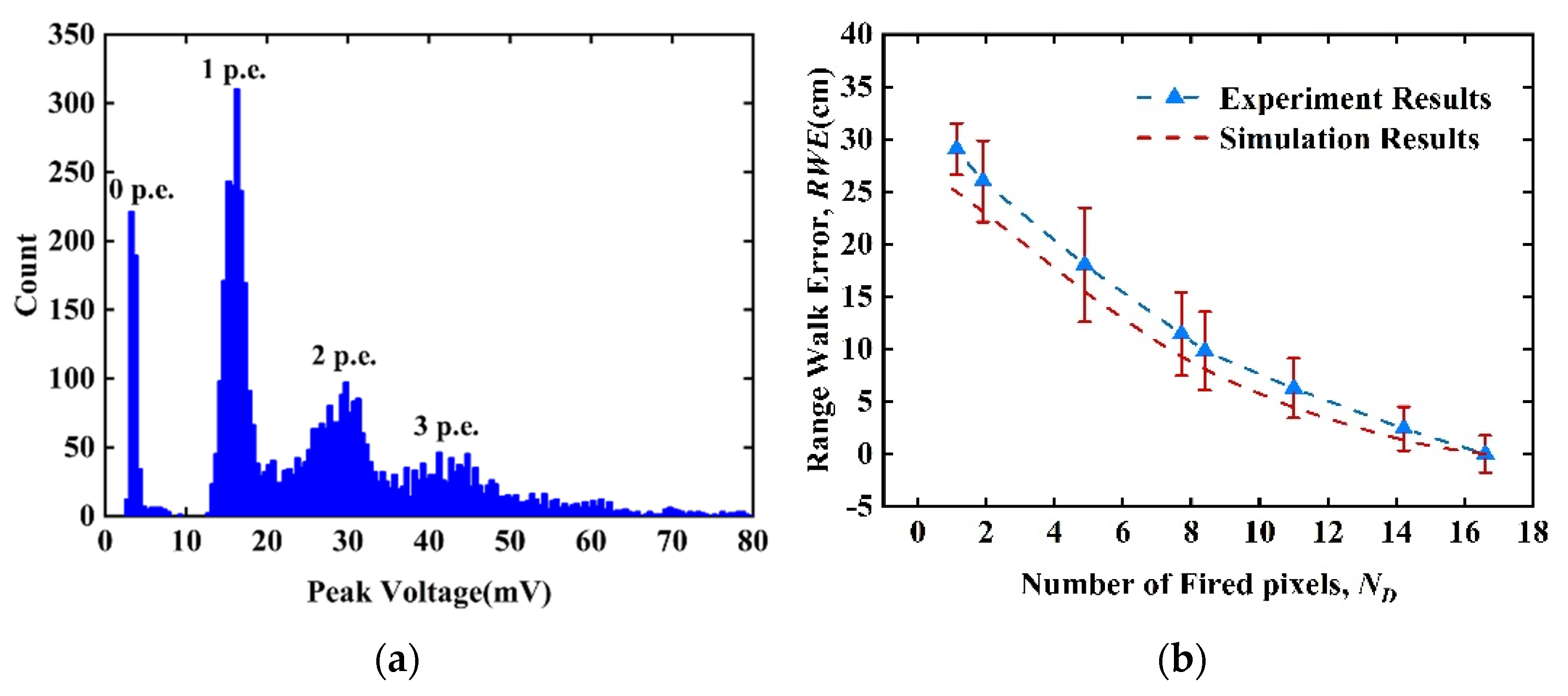
3.1. SiPM Response Measurement

The voltage of the analog SiPM signal is proportional to the number of fired pixels. Figure 5 is obtained by setting the oscilloscope to the glow mode under the condition that the echo signal is a few photons. The brighter the color, the higher the frequency of the signal voltage distribution in the area. This indicates that the voltage of SiPM is discontinuous but discrete. The voltage difference between adjacent bright lines VCell is the peak voltage of the signal that a fired pixel generates. The mean number of fired pixels ND, therefore, can be measured through the peak voltage VPeak generated by SiPM as ND = VPeak/VCell. Then, NS is calculated based on Equation (8). The background noise rate NNoise in the experiment is about 0.005 counts/ns. The noise level is measured in the environment only with background noise. The statistic function of the oscilloscope can count the number of pulses on the screen. By using this function, we count the mean number of false alarm pulses appearing on the screen N. Then, the noise rate is calculated as N/T, where T is the time span of the screen. By adjusting the laser power, the echo light is attenuated to the order of a few photons, and the voltage of SiPM is measured by the oscilloscope.

3.2. Background Noise Measurement

As the SiPM’s signal is the summation of each pixel, an appropriate photon threshold can effectively avoid the false alarms caused by ambient photons and dark counts. The threshold voltage determines the number of photons that activate the TDC. Figure 6a shows the triggered time tag distribution when setting the detection threshold to one-photon and three-photon levels in the laboratory environment. Compared with Figure 6a, the false alarm rate of Figure 6b is significantly reduced, as the background noise mainly causes <3 pixels response [28]. Figure 6c shows that the detection precision is positively correlated with the threshold. However, in practice, choosing the threshold photon number creates a trade-off, with a higher threshold improving the SNR while lowering the probability of successful detection [13]. In the following experiment, we set the threshold photon number as 3 to avoid most of the false alarms and to guarantee the detection probability.

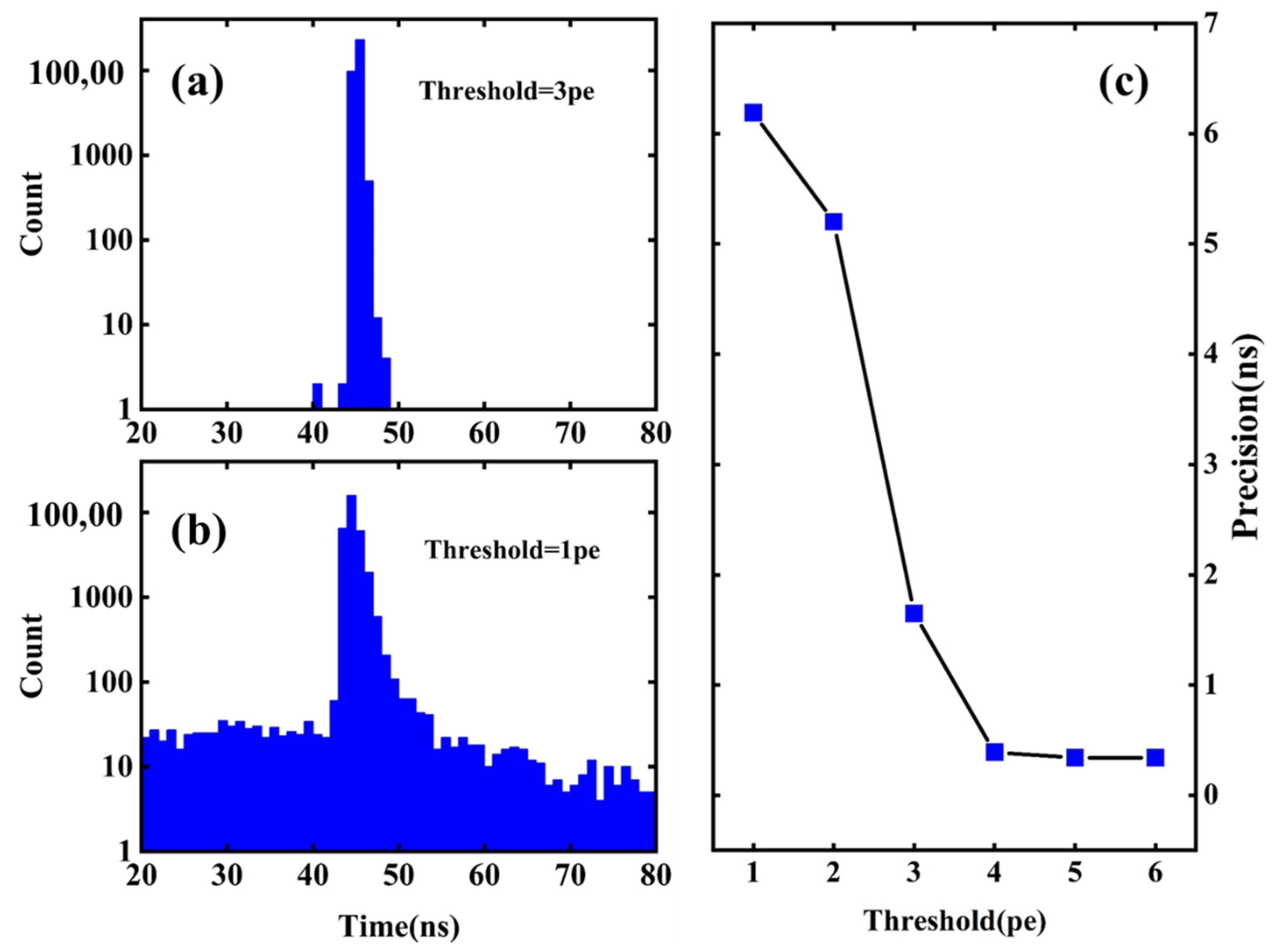
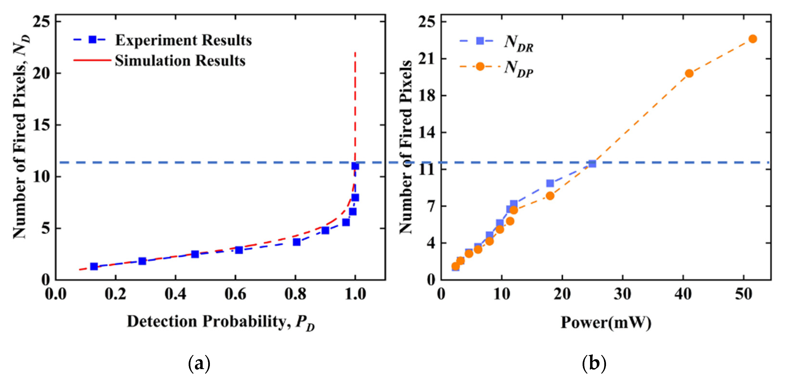
3.3. TOF Measurement

The SiPM LiDAR using photon threshold detection suffers from RWE when the number of received photons fluctuates as seen in Figure 3. Experiments are performed to verify the effectiveness of the RWE correction method we proposed.
Fourteen groups of distance measurement data are obtained under different echo signal intensities, with the ND varying from 1.30 to 46.45. Here, we adjust the power of the semiconductor laser diode to achieve the number fluctuation of the received photons. The experiments are performed for the attenuation rates of 1/1000. The distance between the target and the system is 5.61 m, measured by a phase laser rangefinder (GLM-25, Bosch Shanghai, China) with a precision of 1.5 mm.
In each group, the fixed threshold with k = 3, the CFD method and the PKD method are separately utilized to measure the distance to the same target. As seen in Figure 7a, the three methods are realized through the measurement functions in the oscilloscope, which is controlled by python script through VISA COM [29]. The flight time using the threshold method, TTH, is obtained through the function TVOLT, which measures the time interval between the trigger event and the 2.5 p.e. voltage level on the SiPM signal. The flight time using the CFD method, TCFD, is obtained through the function DELTatime, which measures the time interval from the first specified edge on the trigger event to the next specified edge on the SiPM signal. The flight time using the PKD method, TPKD, is obtained through the function TMAX, which measures the first time at which the maximum voltage of the source waveform occurs. The distance is calculated by aggregating 8000 measurements for each method. Meanwhile, within the measurement using the fixed threshold method, the peak voltage of SiPM is measured, and the detection probability PD is calculated. The relationship between the peak voltage, detection probability and the power of the laser is shown in Figure 7b. It indicates that the detection probability is positively correlated with the emitted power of the laser. Moreover, the peak voltage of SiPM has an approximately linear relationship with the laser power, which is consistent with Equations (3) and (8). When the optical power continues to increase, the detection probability approaches 1. ND is calculated through the peak voltage of SiPM as ND = VPeak/VCell. Then, NS is obtained through Equation (8).
After obtaining the value of ND, a theoretical RWE based on Equation (14) is calculated with TRef = TSim (ND = 46.5). Figure 7c shows the overall RWE correction process. Figure 8 shows the experiment and simulation results of the 14 groups. The results indicate that the RWE between ND = 1.30 and ND = 46.45 is 36.57 cm using the fixed threshold method. As the triggered time of ND = 46.45 is chosen as the reference time, the measurements with a weaker echo signal have a longer triggered time. Therefore, the RWE is positive using the fixed threshold method. By subtracting the simulation results from the experimental results using the fixed threshold method, the RWE is reduced as presented in Figure 9c. The mean RWE after correction is 1.95 cm compared with 7.91 cm using the CFD method and 18.91 cm using the PKD method. As seen in Table 1 below, the proposed RWE correction method shows better performance in improving system accuracy compared with the CFD method and the PKD method. To verify that the proposed technique is valid with different types of SiPMs, the Appendix A includes a set of TOF measurement experiments using the latest detector with high PDE.
The precision in Table 1 shows that the precision of ND with aggregate 100 repetitive measurements is within 0.25 counts, and the ranging precision with aggregate 100 repetitive measurements is within 1.4 cm at the few-photon level. The results indicate that the method does not require thousands of repeated measurements. Therefore, the method is available in wide dynamic LIDAR applications, such as autonomous driving and fast-moving target detection.
Moreover, as the peak voltage measurement requires an extra circuit, considering the simplicity of the LiDAR system, there is another method to calculate ND with no extra system design required. According to Equation (12), the whole detection probability of one shot with the threshold photon number k can be calculated. The detection probability PD is only related to the intensity of echo signal photons under certain instrument parameters. The simulation between ND and PD is performed based on Equation (12) with the same parameters of the above experiments. Meanwhile, we calculate the PD of the above 14 group measurements using the fixed threshold method. PD is the ratio of the number of successful detections to the number of total measurements. The result is as shown in Figure 5. The black dots are the experiment results. It indicates that the simulation can predict the relationship between ND and PD well. Then, ND can be estimated by the simulation function we obtained in Figure 8a. The ND obtained from SiPM’s peak voltage is expressed as NDP, and the ND obtained from the detection probability based on Equation (12) is NDR. Figure 8a depicts the trend of NDP and NDR with the optical power. As seen in Figure 8b, when the ND is less than 12, the result of NDR is close to that of NDP. However, when ND becomes larger, the PD approaches 1 according to Figure 8a. The Δ N D R / Δ P D in Figure 8a becomes very large, which means that the error when measuring PD may induce a huge error when estimating NDR. Considering the restriction of the number of times repeated measurements can be taken, the experimental PD may deviate from the true PD; thus, it is not appropriate to estimate ND when the number of echo photons is large. As a result, ND can be calculated through PD in few-photon detection.

4. Conclusions

For the challenge of RWE, which SiPM LiDAR encounters in wide-dynamic-range measurement applications, we propose an RWE correction method based on the Poisson distribution of arrival photons and the photon number resolvability of SiPM. The only input parameter of this method is the mean number of fired pixels, ND, which can be obtained from the signal of SiPM or the detection probability. Experiments are carried out to verify our method. According to the experiment result, the RWE is almost 37 cm when ND varies from 1.3 to 46.5. The mean residual RWE after complementing the correction method is 1.95 cm, which shows better performance compared with the CFD method and the PKD method. The ranging precision with aggregate 100 repetitive measurements is within 1.2 cm at the few-photon level. The above result indicates that the method enables RWE correction in photon threshold LiDAR systems based on SiPM.
In practice, the peak voltage measurement for the picosecond width pulse generated from SiPM requires a complex system design. Considering the simplicity of the correction method, the method based on detection probability to estimate the light intensity requires no additional measuring system and can improve the accuracy within 4 cm when the mean number of fired pixels fluctuates from 1.31 to 11.22. Therefore, this method may be applicable in LiDAR for detection at the few-photon level.

Author Contributions

Conceptualization, R.Y. and Y.T.; software, R.Y.; validation, R.Y., Y.T. and Z.F.; formal analysis, R.Y.; investigation, K.L., J.Q.; resources, K.L., Z.F.; data curation, R.Y.; writing—original draft preparation, R.Y.; writing—review and editing, R.Y., K.L.; visualization, R.Y.; supervision, K.L., J.Q.; project administration, R.Y.; funding acquisition, K.L., J.Q. All authors have read and agreed to the published version of the manuscript.

Funding

This research was funded by Fudan University and Changchun Institute of Optics Joint Foundation: Grant FC2017-002; Fudan University Innovation Foundation: Grant Y18112.

Conflicts of Interest

The authors declare no conflict of interest.

Appendix A

TOF Measurement with 9% PDE (Photon Detection Efficiency) SiPM

To verify that the proposed technique is valid with different types of SiPMs, the Appendix Section includes a set of TOF measurement experiments using the latest detector with high PDE. We change the detector from SiPM (S13720-1325SA, HAMAMATSU) to SiPM (S15639-1325PS, HAMAMATSU, SiPM module from Gudatek, Hefei, China). The comparison of the two types of SiPM is as shown in Table A1, and their photos are included in Figure A1a.
Table A1. Comparison of the two types of SiPM.
ParameterS15639-1325PSS13720-1325CS
PDE (905 nm)9%7%
Dark count rate0.7 MHz0.5 MHz
Crosstalk probability6%6%
Rise time500 ps500 ps
Gain1.7 × 1061.1 × 106
Number of microcells21202668
Figure A1. (a) The two SiPM modules with S13720-1325CS (left) and S15639-1325PS (right) inside. (b) Experimental platform.
Photonics 09 00024 g0a1
The experimental platform is as shown in Figure A1b. The schematic of the system and the experimental devices is introduced in the manuscript. Eight groups of distance measurement data are obtained under different echo signal intensities, with the ND varying from 1.1 to 16.6. Here, we adjust the power of the semiconductor laser diode from 0.63 W to 13.83 W to achieve the number fluctuation of received photons. Meanwhile, within the measurement using the fixed threshold method, the peak voltage of SiPM is measured as seen in Figure A2a. After obtaining the value of ND, a theoretical RWE based on Equation (14) is calculated, with NCell = 2120, ηq = 9% and TRef = TSim (ND = 16.68). Figure A2b shows the experiment and simulation results of RWE.
Figure A2. (a) Peak voltage of SiPM distribution at ND = 1.91. (b) Experiment and simulation results of RWE.
Photonics 09 00024 g0a2
In our current work, the proposed RWE models take the PDE of the detector into account according to Equations (5) and (6). The result of the TOF measurements using the 9% PDE SiPM in Table A2 shows that the method reduces the RWE from 29.07 cm to the mean deviation of 2.33 cm, with the number of detected photons fluctuating from 1.1 to 16.6. Therefore, the method is proved to be effective for reducing the RWE emerging in the SiPM LiDAR with 9% PDE, and the proposed model can accurately predict the response characteristics of different SiPMs.
Table A2. Accuracy results with different echo signal intensities.
ND1.13 1.91 4.887.72 8.4011.0014.22
ETH (cm)29.07 26.0018.0311.43 9.816.26 2.42
ETHC (cm)4.072.862.542.151.841.751.08
ETH: RWE of threshold method. ETHC: Corrected RWE.

References

  1. Albota, M.A.; Heinrichs, R.M.; Kocher, D.G.; Fouche, D.G.; Player, B.E.; O’Brien, M.E.; Aull, B.F.; Zayhowski, J.J.; Mooney, J.; Willard, B.C.; et al. Three-dimensional imaging laser radar with a photon-counting avalanche photodiode array and microchip laser. Appl. Opt. 2002, 41, 7671–7678. [Google Scholar] [CrossRef] [Green Version]
  2. Tachella, J.; Altmann, Y.; Mellado, N.; McCarthy, A.; Tobin, R.; Buller, G.S.; Tourneret, J.-Y.; McLaughlin, S. Real-time 3D reconstruction from single-photon lidar data using plug-and-play point cloud denoisers. Nat. Commun. 2019, 10, 4984. [Google Scholar] [CrossRef] [PubMed] [Green Version]
  3. Li, Z.P.; Ye, J.T.; Huang, X.; Jiang, P.Y.; Cao, Y.; Hong, Y.; Yu, C.; Zhang, J.; Zhang, Q.; Peng, C.Z. Single-photon imaging over 200 km. Optica 2021, 8, 344. [Google Scholar] [CrossRef]
  4. Johnson, S.; Gatt, P.; Nichols, T. Analysis of Geiger-mode APD laser radars. In Proceedings of the Laser Radar Technology and Applications VIII, Orlando, FL, USA, 21 August 2003. [Google Scholar]
  5. Liang, Y.; Huang, J.; Ren, M.; Feng, B.; Chen, X.; Wu, E.; Wu, G.; Zeng, H. 1550-nm time-of-flight ranging system employing laser with multiple repetition rates for reducing the range ambiguity. Opt. Express 2014, 22, 4662–4670. [Google Scholar] [CrossRef] [Green Version]
  6. Massa, J.S.; Buller, G.S.; Walker, A.C.; Cova, S.; Umasuthan, M.; Wallace, A.M. Time-of-flight optical ranging system based on time-correlated single-photon counting. Appl. Opt. 1998, 37, 7298–7304. [Google Scholar] [CrossRef] [Green Version]
  7. Buller, G.; Wallace, A. Ranging and Three-Dimensional Imaging Using Time-Correlated Single-Photon Counting and Point-by-Point Acquisition. IEEE J. Sel. Top. Quantum Electron. 2007, 13, 1006–1015. [Google Scholar] [CrossRef] [Green Version]
  8. Bao, Z.; Liang, Y.; Wang, Z.; Li, Z.; Wu, E.; Wu, G.; Zeng, H. Laser ranging at few-photon level by photon-number-resolving detection. Appl. Opt. 2014, 53, 3908–3912. [Google Scholar] [CrossRef]
  9. Buzhan, P.; Dolgoshein, B.; Filatov, L.; Ilyin, A.; Kantzerov, V.; Kaplin, V.; Karakash, A.; Kayumov, F.; Klemin, S.; Popova, E.; et al. Silicon photomultiplier and its possible applications. Nucl. Instrum. Methods Phys. Res. A 2003, 504, 48–52. [Google Scholar] [CrossRef]
  10. Collazuol, G.; Ambrosi, G.; Boscardin, M.; Corsi, F.; Betta, G.; Guerra, A.D.; Dinu, N.; Galimberti, M.; Giulietti, D.; Gizzi, L.A. Single photon timing resolution and detection efficiency of the IRST silicon photo-multipliers. Nucl. Instrum. Methods Phys. Res. A 2007, 581, 461–464. [Google Scholar] [CrossRef]
  11. Villa, F.; Severini, F.; Madonini, F.; Zappa, F. SPADs and SiPMs Arrays for Long-Range High-Speed Light Detection and Ranging (LiDAR). Sensors 2021, 21, 3839. [Google Scholar] [CrossRef]
  12. Haemisch, Y.; Frach, T.; Degenhardt, C.; Thon, A. Fully Digital Arrays of Silicon Photomultipliers (dSiPM)—A Scalable Alternative to Vacuum Photomultiplier Tubes (PMT). Phys. Procedia 2012, 37, 1546–1560. [Google Scholar] [CrossRef] [Green Version]
  13. Cohen, L.; Matekole, E.S.; Sher, Y.; Istrati, D.; Eisenberg, H.S.; Dowling, J.P. Thresholded quantum LIDAR: Exploiting photon-number-resolving detection. Phys. Rev. Lett. 2019, 123, 203601. [Google Scholar] [CrossRef] [Green Version]
  14. Yue, M.; Song, L.; Zhang, W.; Zhang, Z.; Liu, R.; Hua, W.X. Theoretical ranging performance model and range walk error correction for photon-counting lidars with multiple detectors. Opt. Express 2018, 26, 15924. [Google Scholar]
  15. Xu, L.; Zhang, Y.; Zhang, Y.; Yang, C.; Yang, X.; Zhao, Y. Restraint of range walk error in a Geiger-mode avalanche photodiode lidar to acquire high-precision depth and intensity information. Appl. Opt. 2016, 55, 1683–1687. [Google Scholar] [CrossRef]
  16. He, W.; Sima, B.; Chen, Y.; Dai, H.; Chen, Q.; Gu, G. A correction method for range walk error in photon counting 3D imaging LIDAR. Opt. Commun. 2013, 308, 211–217. [Google Scholar] [CrossRef]
  17. Min, S.O.; Hong, J.K.; Kim, T.H.; Hong, K.H.; Kim, B.W. Reduction of range walk error in direct detection laser radar using a Geiger mode avalanche photodiode. Opt. Commun. 2010, 283, 304–308. [Google Scholar]
  18. Chen, Z.; Li, X.; Li, X.; Ye, G.; Zhou, Z.; Lu, L.; Sun, T.; Fan, R.; Chen, D. A correction method for range walk error in time-correlated single-photon counting using photomultiplier tube. Opt. Commun. 2019, 434, 7–11. [Google Scholar] [CrossRef]
  19. Kilpel, A.; Ylitalo, J.; Mtt, K.; Kostamovaara, J. Timing discriminator for pulsed time-of-flight laser rangefinding measurements. Rev. Sci. Instrum. 1998, 69, 1978–1984. [Google Scholar] [CrossRef] [Green Version]
  20. Du, J.; Schmall, J.P.; Judenhofer, M.S.; Di, K.; Cherry, S.R. A Time-Walk Correction Method for PET Detectors Based on Leading Edge Discriminators. IEEE Trans. Radiat. Plasma Med. Sci. 2017, 1, 385. [Google Scholar] [CrossRef]
  21. Li, X.; Yang, B.; Xie, X.; Li, D.; Xu, L. Influence of waveform characteristics on LiDAR ranging accuracy and precision. Sensors 2018, 18, 1156. [Google Scholar] [CrossRef] [Green Version]
  22. Johnson, E.S. Effect of target surface orientation on the range precision of laser detection and ranging systems. J. Appl. Remote Sens. 2009, 3, 2527–2532. [Google Scholar] [CrossRef]
  23. Lim, H.C.; Zhang, Z.P.; Sung, K.P.; Park, J.U.; Choi, M. Modeling and Analysis of an Echo Laser Pulse Waveform for the Orientation Determination of Space Debris. Remote Sens. 2020, 12, 1659. [Google Scholar] [CrossRef]
  24. Kostamovaara, J.; Huikari, J.; Hallman, L.; Nissinen, I.; Nissinen, J.; Rapakko, H.; Avrutin, E.; Ryvkin, B. On Laser Ranging Based on High-Speed/Energy Laser Diode Pulses and Single-Photon Detection Techniques. IEEE Photonics J. 2015, 7, 1–15. [Google Scholar] [CrossRef]
  25. Daniel, G.F. Detection and false-alarm probabilities for laser radars that use Geiger-mode detectors. Appl. Opt. 2003, 42, 5388–5398. [Google Scholar]
  26. Renker, D.; Lorenz, E. Advances in solid state photon detectors. J. Instrum. 2009, 4, P04004. [Google Scholar] [CrossRef]
  27. Chen, L.H. On the convergence of Poisson binomial to Poisson distributions. Ann. Probab. 1974, 2, 178–180. [Google Scholar] [CrossRef]
  28. Tang, Y.; Yang, R.; Qiu, J.; Liu, K. Wide dynamic laser ranging based on diode laser and photon-counting techniques. Appl. Opt. 2021, 60, 2716–2721. [Google Scholar] [CrossRef]
  29. Keysight Infiniium Oscilloscopes Programmer’s Guide. Available online: https://www.etesttool.com/downloads/pdf/Keysight/Keysight-DSAZ634A/Infiniium_prog_guide.pdf (accessed on 23 December 2021).
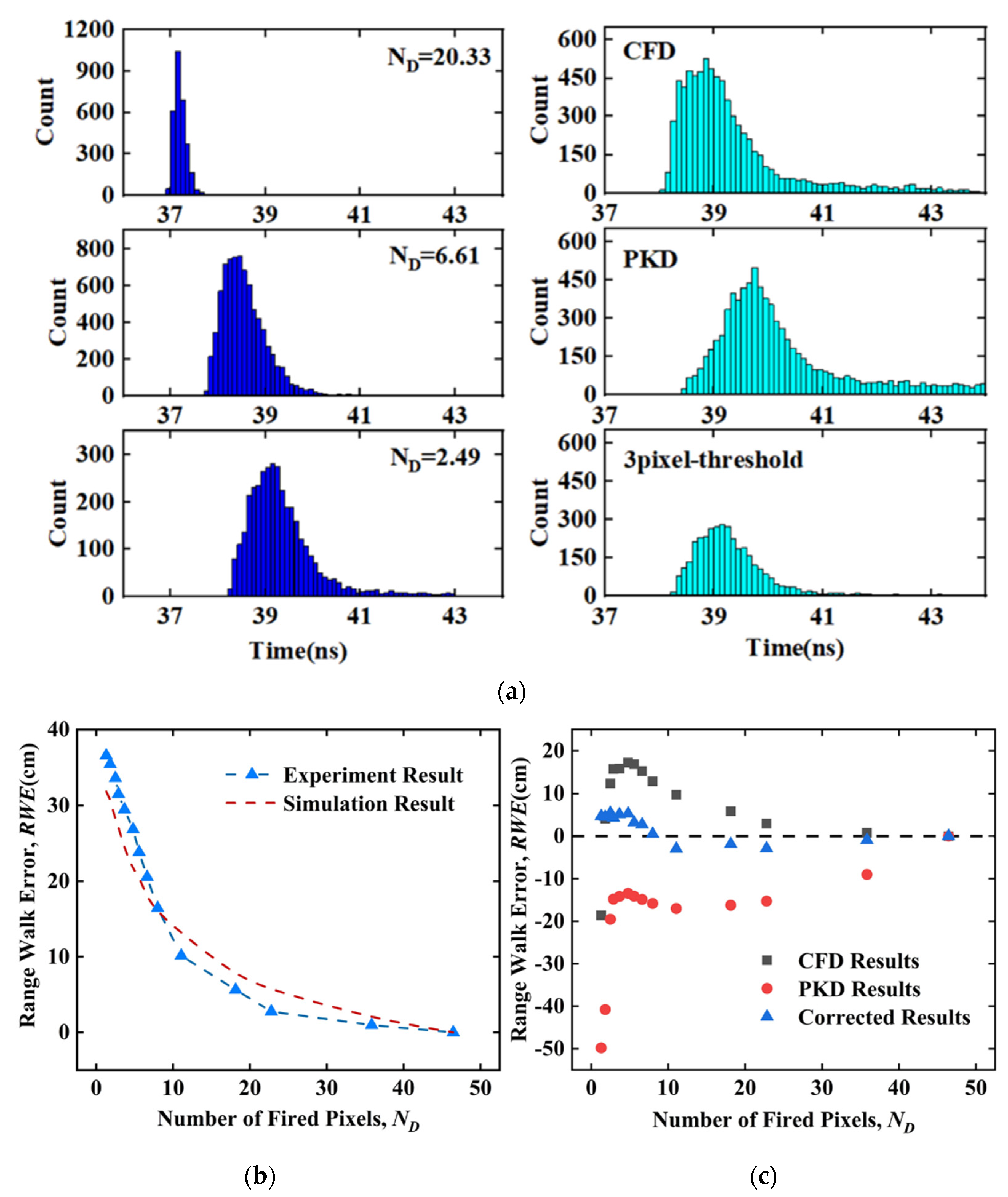
Figure 1. The mean number of fired pixels, ND, versus the mean number of received photons, NS, with different number of pixels in SiPM, NCell.
Photonics 09 00024 g001
Figure 2. Detection probability under different circumstances: (a) echo light intensities and (b) FWHM of the laser pulse.
Photonics 09 00024 g002
Figure 3. (a) Simulation result between RWE and mean number of fired pixels with different thresholds. (b) Detection probability between fired pixels with different thresholds.
Photonics 09 00024 g003
Figure 4. (a) Schematic of the LiDAR system based on SiPM. (b) Experimental platform.
Photonics 09 00024 g004aPhotonics 09 00024 g004b
Figure 5. SiPM output signal measured by the oscilloscope in glow mode.
Photonics 09 00024 g005
Figure 6. (a,b) Triggered time tag distribution of 3 p.e. and 1 p.e. detection threshold. (c) Relationship between system precision and threshold.
Photonics 09 00024 g006
Figure 7. (a) The oscilloscope waveform of time-of-flight measurement with the markers of the measured time using fixed threshold, CFD and PKD methods. (b) Peak voltage of SiPM and detection probability versus optical power. (c) Schematic diagram of range walk error restraint.
Photonics 09 00024 g007
Figure 8. (a) Simulation and experiment results of detection probability versus mean number of fired pixels based on Equation (13). (b) ND derived from peak voltage and detection probability versus optical power.
Photonics 09 00024 g008
Figure 9. (a) Triggered time tag distribution using fixed threshold method with different mean number of fired pixels, N D (left), and triggered time tag distribution using three methods with N D = 2.48 (right). (b) Experiment and simulation result of RWE. The dashed line is the simulation result; the blue triangles are the experiment results of fixed threshold method. (c) Correction results of the three methods. The blue triangles are the error after applying the correction method; the black squares are the CFD results; the red spots are the PKD results.
Photonics 09 00024 g009
Table 1. Accuracy result and precision of different echo signal intensities with 100 repetitive measurements (part of).
ND2.884.797.9818.1433.65
ETH (cm)31.5226.8616.455.650.97
ECFD (cm)15.7417.2112.805.830.79
EPKD (cm)−19.54−13.44−15.83−16.23−9.02
ETHC (cm)4.345.300.51−1.85−0.91
Precision (cm)1.191.111.310.270.21
ETH: RWE of threshold method. ECFD: RWE of CFD method. EPKD: RWE of PKD method. ETHC: Corrected RWE.
Publisher’s Note: MDPI stays neutral with regard to jurisdictional claims in published maps and institutional affiliations.

