Fast Measurement of Brillouin Frequency Shift in Optical Fiber Based on a Novel Feedforward Neural Network


Abstract
:1. Introduction
2. Theory
2.1. PCA
2.2. FNN
- The input vector is [];
- The input and output of unit in the hidden layer is and , respectively;
- The weight from jth unit in the previous layer to ith in the next layer is ;
- The output value is .
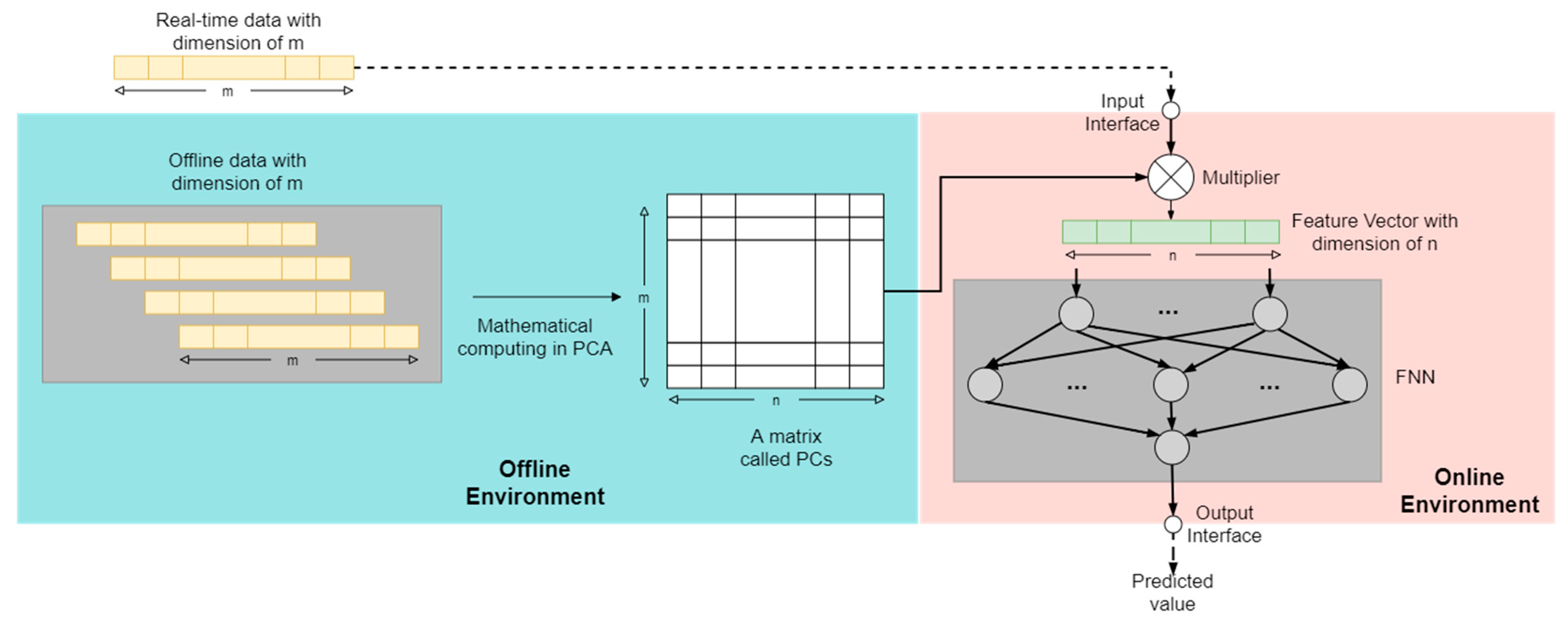
2.3. FNN with PCA
3. Proposed Method
4. Results
4.1. Simulation Results
4.2. Experimental Results
5. Conclusions
Author Contributions
Funding
Institutional Review Board Statement
Informed Consent Statement
Data Availability Statement
Acknowledgments
Conflicts of Interest
References
- Thoben, K.-D.; Wiesner, S.; Wuest, T. “Industrie 4.0” and Smart Manufacturing—A Review of Research Issues and Application Examples. Int. J. Autom. Technol. 2017, 11, 4–16. [Google Scholar] [CrossRef] [Green Version]
- Wang, J.; Ma, Y.; Zhang, L.; Gao, R.X.; Wu, D. Deep learning for smart manufacturing: Methods and applications. J. Manuf. Syst. 2018, 48, 144–156. [Google Scholar] [CrossRef]
- Bandyopadhyay, D.; Sen, J. Internet of Things: Applications and Challenges in Technology and Standardization. Wirel. Pers. Commun. 2011, 58, 49–69. [Google Scholar] [CrossRef]
- Feng, C.; Schneider, T. Benefits of Spectral Property Engineering in Distributed Brillouin Fiber Sensing. Sensors 2021, 21, 1881. [Google Scholar] [CrossRef] [PubMed]
- Horiguchi, T.; Tateda, M. Optical-fiber-attenuation investigation using stimulated Brillouin scattering between a pulse and a continuous wave. Opt. Lett. 1989, 14, 408–410. [Google Scholar] [CrossRef] [PubMed]
- Lopez-Gil, A.; Dominguez-Lopez, A.; Martin-Lopez, S.; Gonzalez-Herraez, M. Simple Method for the Elimination of Polarization Noise in BOTDA Using Balanced Detection and Orthogonal Probe Sidebands. J. Light. Technol. 2014, 33, 2605–2610. [Google Scholar] [CrossRef]
- Peled, Y.; Motil, A.; Tur, M. Fast Brillouin optical time domain analysis for dynamic sensing. Opt. Express 2012, 20, 8584–8591. [Google Scholar] [CrossRef] [PubMed]
- Voskoboinik, A.; Willner, A.E.; Tur, M. Extending the dynamic range of sweep-free Brillouin optical time-domain analyzer. J. Light. Technol. 2015, 33, 1. [Google Scholar] [CrossRef]
- Voskoboinik, A.; Wang, J.; Shamee, B.; Nuccio, S.R.; Zhang, L.; Chitgarha, M.; Willner, A.E.; Tur, M. SBS-Based Fiber Optical Sensing Using Frequency-Domain Simultaneous Tone Interrogation. J. Light. Technol. 2011, 29, 1729–1735. [Google Scholar] [CrossRef]
- Jin, C.; Guo, N.; Feng, Y.; Wang, L.; Liang, W.; Li, J.; Li, Z.; Yu, C.; Lu, C. Scanning-free BOTDA based on ultra-fine digital optical frequency comb. Opt. Express 2015, 23, 5277–5284. [Google Scholar] [CrossRef] [PubMed]
- Voskoboinik, A.; Yilmaz, O.F.; Willner, A.W.; Tur, M. Sweep-free distributed Brillouin time-domain analyzer (SF-BOTDA). Opt. Express 2011, 19, B842–B847. [Google Scholar] [CrossRef] [PubMed]
- Azad, A.K.; Wang, L.; Guo, N.; Tam, H.Y.; Lu, C. Signal processing using artificial neural network for BOTDA sensor system. Opt. Express 2016, 24, 6769–6782. [Google Scholar] [CrossRef] [PubMed]
- Liang, Y.; Jiang, J.; Chen, Y.; Zhu, R.; Lu, C.; Wang, Z. Optimized Feedforward Neural Network Training for Efficient Brillouin Frequency Shift Retrieval in Fiber. IEEE Access 2019, 7, 68034–68042. [Google Scholar] [CrossRef]
- Azad, A.K.; Khan, F.N.; Al-Arashi, W.; Guo, N.; Lau, A.P.T.; Lu, C. Temperature extraction in Brillouin optical time-domain analysis sensors using principal component analysis based pattern recognition. Opt. Express 2017, 25, 16534–16549. [Google Scholar] [CrossRef] [PubMed]
- Nordin, N.D.; Zan, M.S.D.; Abdullah, F. Comparative Analysis on the Deployment of Machine Learning Algorithms in the Distributed Brillouin Optical Time Domain Analysis (BOTDA) Fiber Sensor. Photonics 2020, 7, 79. [Google Scholar] [CrossRef]
- Aguilera, A.M.; Gutiérrez, R.; Ocaña, F.A.; Valderrama, M.J. Computational approaches to estimation in the principal component analysis of a stochastic process. Appl. Stoch. Model. Data Anal. 1995, 11, 279–299. [Google Scholar] [CrossRef]
- Jolliffe, I.T. Principal Component Analysis, 2rd ed.; Springer: New York, NY, USA, 2002; pp. 150–166. [Google Scholar] [CrossRef]
- Alvin, C.; Rencher, W.F.C. Methods of Multivariate Analysis, 3rd ed.; John Wiley & Sons: Hoboken, NJ, USA, 2021; pp. 169–257. [Google Scholar] [CrossRef]
- LeCun, Y.; Bengio, Y.; Hinton, G. Deep learning. Nature 2015, 521, 436–444. [Google Scholar] [CrossRef] [PubMed]
- Hong, X.; Wu, J.; Li, Y.; Wang, S.; Qiu, J.; Sun, X.; Zhang, X. Data for: A fast method for Brillouin frequency shift estimation. Sens. Actuators A Phys. 2018, 284, 6–11. [Google Scholar] [CrossRef]


| Parameter | Range | Interval | Number of Repetitions |
|---|---|---|---|
| BFS | 10.62–10.98 GHz | 1 MHz | 1 |
| FWHM | 10–60 MHz | 1 MHz | 1 |
| SNR | 10–40 dB | 1 dB | 3 |
| BFSnorm | 5–95% | 1/400 | 51 |
| Parameter | Range | Interval | Number of Repetitions |
|---|---|---|---|
| BFS | 10.62–10.98 GHz | 1 MHz | 1 |
| FWHM | 10–60 MHz | 1 MHz | 1 |
| SNR | - | - | - |
| BFSnorm | 5–95% | 1/400 | 51 |
| FNN Type | MAE | Processing Time 1 |
|---|---|---|
| FNN with PCA | 0.2027 MHz | 1.4224 s |
| FNN without PCA | 0.2329 MHz | 4.5273 s |
| LCF | 0.1816 MHz | 886 s |
| Frequency Scanning Step | MAE |
|---|---|
| 5 MHz | 1.1968 MHz |
| 2 MHz | 0.2027 MHz |
| 1 MHz | 0.4888 MHz |
| The ith Frequency Scanning Step | The jth Frequency Scanning Step | S(i, j) |
|---|---|---|
| 1 MHz | 2 MHz | 0.0150 |
| 1 MHz | 5 MHz | 0.0377 |
| 2 MHz | 5 MHz | 0.0316 |
Publisher’s Note: MDPI stays neutral with regard to jurisdictional claims in published maps and institutional affiliations. |
© 2021 by the authors. Licensee MDPI, Basel, Switzerland. This article is an open access article distributed under the terms and conditions of the Creative Commons Attribution (CC BY) license (https://creativecommons.org/licenses/by/4.0/).
Share and Cite
Xiao, F.; Lv, M.; Li, X. Fast Measurement of Brillouin Frequency Shift in Optical Fiber Based on a Novel Feedforward Neural Network. Photonics 2021, 8, 474. https://doi.org/10.3390/photonics8110474
Xiao F, Lv M, Li X. Fast Measurement of Brillouin Frequency Shift in Optical Fiber Based on a Novel Feedforward Neural Network. Photonics. 2021; 8(11):474. https://doi.org/10.3390/photonics8110474
Chicago/Turabian StyleXiao, Fen, Mingxing Lv, and Xinwan Li. 2021. "Fast Measurement of Brillouin Frequency Shift in Optical Fiber Based on a Novel Feedforward Neural Network" Photonics 8, no. 11: 474. https://doi.org/10.3390/photonics8110474