Article

Study on Transmission Characteristics and Bandgap Types of Plasma Photonic Crystal

1
School of Aerospace Engineering, Xiamen University, Xiamen 361102, China
2
Fujian Key Laboratory of Plasma and Magnetic Resonance Research, Xiamen 361102, China
*
Author to whom correspondence should be addressed.
Photonics 2021, 8(9), 401; https://doi.org/10.3390/photonics8090401
Submission received: 11 August 2021 / Revised: 6 September 2021 / Accepted: 8 September 2021 / Published: 20 September 2021
(This article belongs to the Special Issue Photonic Devices and Systems)

Abstract

:
A plasma photonic crystal (PPC) was formed using an array of discharge plasma tubes. The transmission spectra and bandstructure of PPCs with different lattice types under different polarization modes were studied through simulation and measurement. To study the types of bandgap in PPCs, the bandstructure of the PPC is calculated using symplectic finite difference time domain (SFDTD), a modified plane wave expansion (PWE) method, and a finite element method (FEM) based on weak form equations. The bandstructure of the PPC is compared with the transmission curve results. The results show that the bandgap is stable in the PPC, and the experimental and numerical results of the transmission spectra agree well. There are different types of bandgap in the PPC; the bandgap under TE-like polarization is caused by localized surface plasmon (LSP) and Bragg scattering. The bandgap under TM-like polarization is caused by the cutoff effect of plasma on the electromagnetic wave and Bragg scattering. The lattice type also affects the position and number of the bandgap. The three methods have their advantages and disadvantages when calculating bandstructure. Therefore, it is necessary to combine the results of three methods and experimental results to accurately determine the bandgap type of the PPC.

1. Introduction

Plasma photonic crystals (PPCs) composed of plasma arrays not only have the properties of conventional photonic crystals (PCs), but can also change their dielectric constant by controlling the plasma parameters (electron density, collision frequency, etc.), thereby having a tunable photonic bandgap (PBG). In addition, PPCs can generate a localized surface plasmon (LSP) bandgap in specific polarization mode; the LSP bandgap will have a strong absorption effect on electromagnetic waves, and the LSP bandgap is also tunable. Therefore, PPCs can be used to construct electromagnetic wave absorbing devices easily. It has broad application prospects. In the future, PPCs are expected to be used in electromagnetic cloaking devices, microwave isolators, omnidirectional reflectors, and other microwave devices.
Since the concept of PPCs was proposed, its transmission characteristics have been the focus of research. Sakai et al. first proposed the concept of PPCs, constructed a helium discharge plasma array at atmospheric pressure, and investigated the bandgap of PPCs by experimental tests and numerical calculations [1,2]; Fan [3] and Wang et al. [4], used dielectric barrier discharge (DBD) with two water electrodes to obtain a two-dimensional PPC with tunable lattice arrangement and photonic bandgap; Wang et al. [5] designed a three-dimensional woodpile type PPC and calculated and tested its transmission characteristics; Zhang [6], Wen [7], and Wang [8] composed a PPC using plasma discharge tubes and tested and calculated its transmission and absorption characteristics; V. I. Arkhipenko et al. [9] obtained PPCs using neon glow discharge arrays, placed them in waveguides, and studied the transmission characteristics of PPCs at X-band; V. S. Babitski [10] obtained a PPC using argon pulse discharge at atmospheric pressure and also calculated and tested the transmission characteristics of PPCs. The results show that the properties of PPCs are similar to those of metallic photonic crystals at high electron density. Akinori et al. [11] constructed a periodic array structure using double split ring resonators and plasma discharge tubes, and the results showed that the structure has negative magnetic permeability, which means the tunable negative-refractive-index device can be achieved. Wang et al. [12] composed a photonic crystal using spherical silicon nitride and plasma discharge tubes and discussed how such photonic crystals can be applied in photonic artificial neural networks and optical computing systems.
In recent years, the study of the transmission characteristics of PPCs has been fruitful, but not much literature has been published on the analysis of the PPC bandgap type. Righetti [13], Tan [14], etc. determined the bandgap type by the transmission spectra and dielectric constant of plasma. In the author’s opinion, more powerful evidence is needed to determine the bandgap type.
In this paper, two different lattice types of PPCs are constructed using plasma discharge tubes, a model for calculating PPCs is established, and the transmission spectra of PPCs under different polarization modes are experimentally and calculated. To analyze the bandgap types in the PPC transmission spectra, the bandstructure of the PPC is calculated using the symplectic finite difference time domain (SFDTD) and modified plane wave expansion (PWE) methods and finite element method (FEM) base on weak form equations; the types of bandgap in PPC transmission spectra are analyzed based on the computational and experimental results, and the characteristics of the three methods are discussed.
The calculation of the transmission spectra in this paper uses CST Studio software; the details of the PWE method are shown in Appendix A; the details of the weak form equations are shown in Appendix B, and the calculation is completed using COMSOL software; the iterative scheme of SFDTD is shown in Appendix C.
In the experiment, a 7 × 6 (row × column) array of plasma tubes was used to form a PPC with a square lattice and triangular lattice with a lattice constant a = 20 mm, as shown in Figure 1. The plasma tubes were controlled by a set of ballasts based on the DALI control protocol. Each plasma tube was 16 mm in diameter and 260 mm in length, with a mixture of low-pressure argon gas and mercury vapor inside. The walls of the plasma tubes were made of quartz glass with a thickness of 1 mm.
The experiments were conducted in a 6 m (length) × 6 m (width) × 6 m (height) darkroom. A PPC was placed on a low scattering turntable, and the whole test system was placed inside the microwave anechoic chamber. The vector network analyzer used for the measurement is Agilent N5224A, and the antenna is a dual-ridge broadband antenna with an experimental frequency range of 1–12 GHz. The electromagnetic wave propagates negatively along the X-axis, and the polarization directions are Y-direction and Z-direction, respectively. Due to the limited length of the discharge tube in the experiment, the TE polarization and TM polarization here do not satisfy the ideal situation, and for accurate description, the Y-direction polarization is called TE-like polarization and the Z-direction polarization is called TM-like polarization.

2. Transmission Characteristics and Bandstructure of PPC

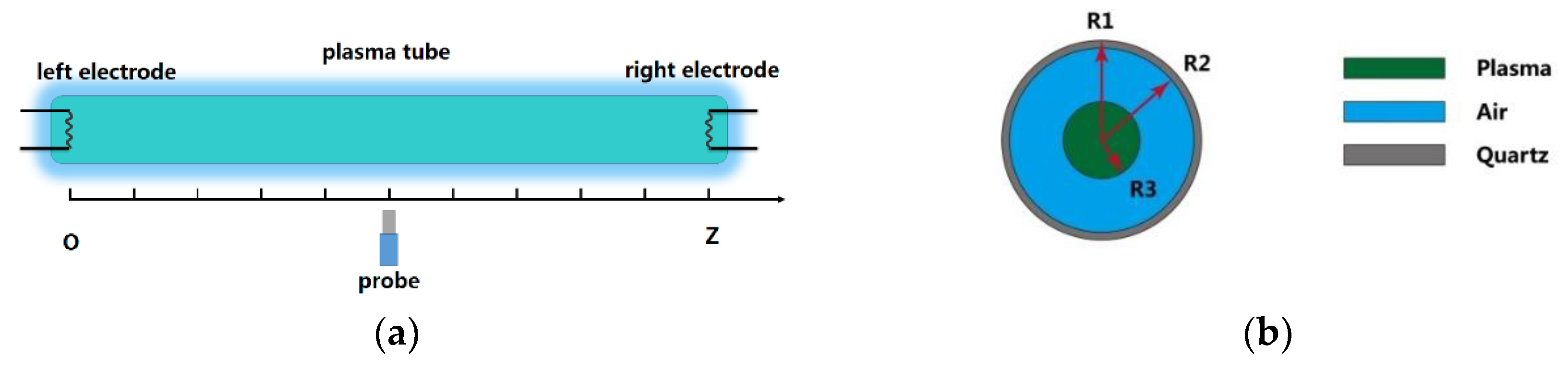
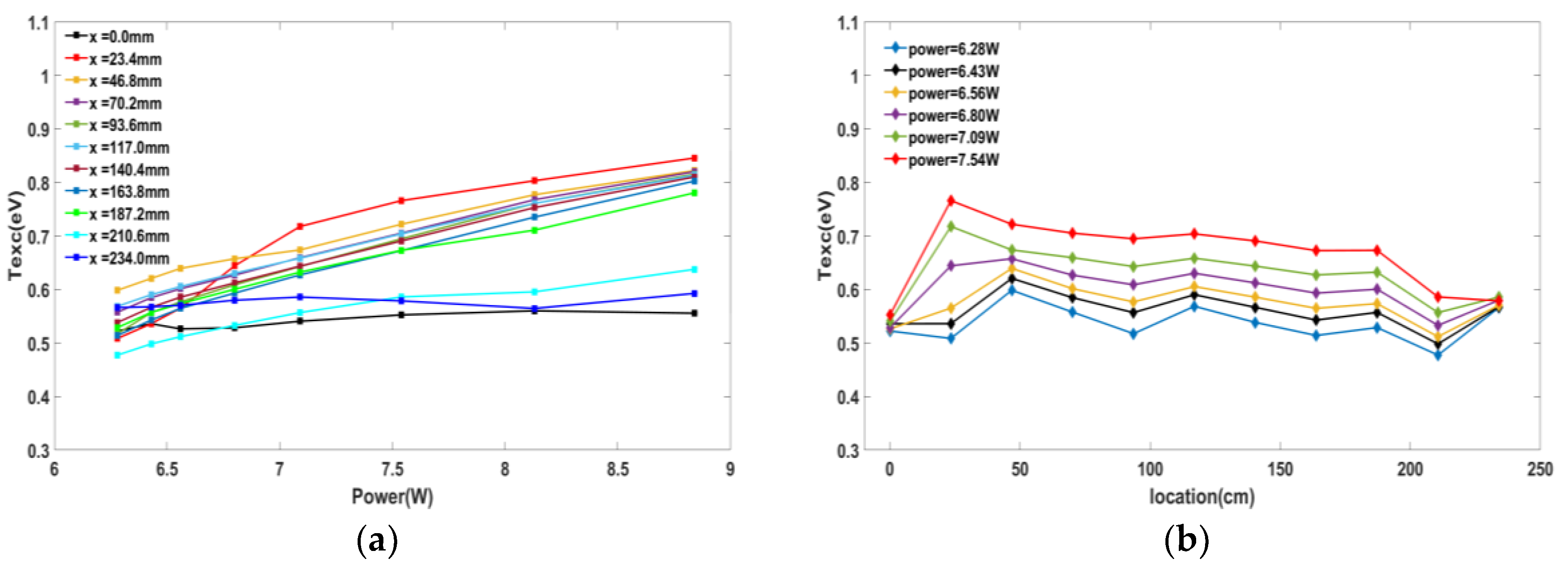
2.1. Modeling of PPC Unit

The plasma distribution in the discharge tube is not uniform. Generally speaking, low-pressure low-temperature plasma usually does not meet local thermodynamic equilibrium (LTE) conditions. Therefore, the Boltzmann spectral lines method cannot be used to estimate the electron temperature. However, the Fermi–Dirac model can be used to diagnose the electron excitation temperature [15], and the trend of the electron excitation temperature is similar to that of the electron temperature, so the change in the electron temperature can be inferred according to the change law of the electron excitation temperature. Walker [16] gave a Fermi–Dirac model for calculating the electron excitation temperature under non-LTE conditions:
ln ( R p ) = ln ( I i j λ i j g i A i j ) = ln [ exp ( ε i μ ) / k T e x c + 1 ] 1 + C
where R p is the relative population, I i j is the measured relative emission intensity, λ i j is the transition wavelength, g i is the upper state statistical weight, A i j is the Einstein coefficient for spontaneous emission, ε i is excitation energy, T e x c is electron excitation temperature, and C is a proportionality constant. Then, the values of parameters T e x c , μ , and C were obtained with the use of nonlinear-curve-fitting method.
The measurement points are shown in Figure 2a. The spectrometer is the HR4000+ produced by Ocean Optics. The spectral data comes from the National Institute of Standards and Technology (NIST) database [17], as given in Table 1. The result of electron excitation temperature in the plasma tube is shown in Figure 3.
Figure 3a shows that as discharge power increases, the electron excitation temperature in the tube also increases. Therefore, it can be considered that the electron temperature also increases. The meaning of electron temperature is the average electron energy, so the power increases, the energy gained by the electrons escaping from the electrode increases, and the electron temperature increases. In a low-pressure glow discharge tube, the electron temperature and electron density have similar changes along the axial direction. Therefore, it can be considered that, when the discharge power increases, the electron density increases. Figure 3b shows that the electron excitation temperature is more uniformly distributed outside the electrode, and the uniformity increases with the increase in power. Since the discharge tube works under AC power, the two electrodes alternately become cathode and anode, so the two electrodes may alternately be in the anode area or cathode area; thus, the electron excitation temperature is different from other areas. While the remaining measurement points are located in the positive column area, and the plasma parameters’ distribution in the positive column area are uniform, so the electron temperature distribution is relatively uniform. Based on this, it can be approximated that the plasma distribution in the axial direction is relatively uniform, and the influence of the axial direction is ignored in the modeling.
In the radial direction, the electron density is largest at the center and zero at the wall. Therefore, an equivalent model is established, as shown in Figure 2b. The outermost layer of the model is quartz glass, the dielectric constant ε is 3.8, the middle layer is air, and the innermost layer is plasma. The radii of each layer are: R1 = 8 mm, R2 = 7 mm, and R3 = 4 mm. The dielectric constant of the plasma uses the Drude model, and the specific formula can be found in reference [8].
The electron density in the low-pressure glow discharge plasma tube is generally considered to be in the range of approximately 1016/m3 to 1018/m3. The order of magnitude of the collision frequency was estimated, using BOLSIG+ software [18], to be 109 Hz. The power consumed by each discharge tube is P1 = 6.28 W, P2 = 6.43 W, and P3 = 6.56 W; the corresponding electron density used for the calculation is: ne1 = 2.64 × 10¹⁷/m3, ne2 = 2.92 × 10¹⁷/m3, and ne3 = 3.36 × 10¹⁷/m3.
As the electron density increases, the collision frequency also increases. Therefore, the collision frequency is, respectively, taken as: v1 = 5 GHz, v2 = 6 GHz, and v3 = 8 GHz.

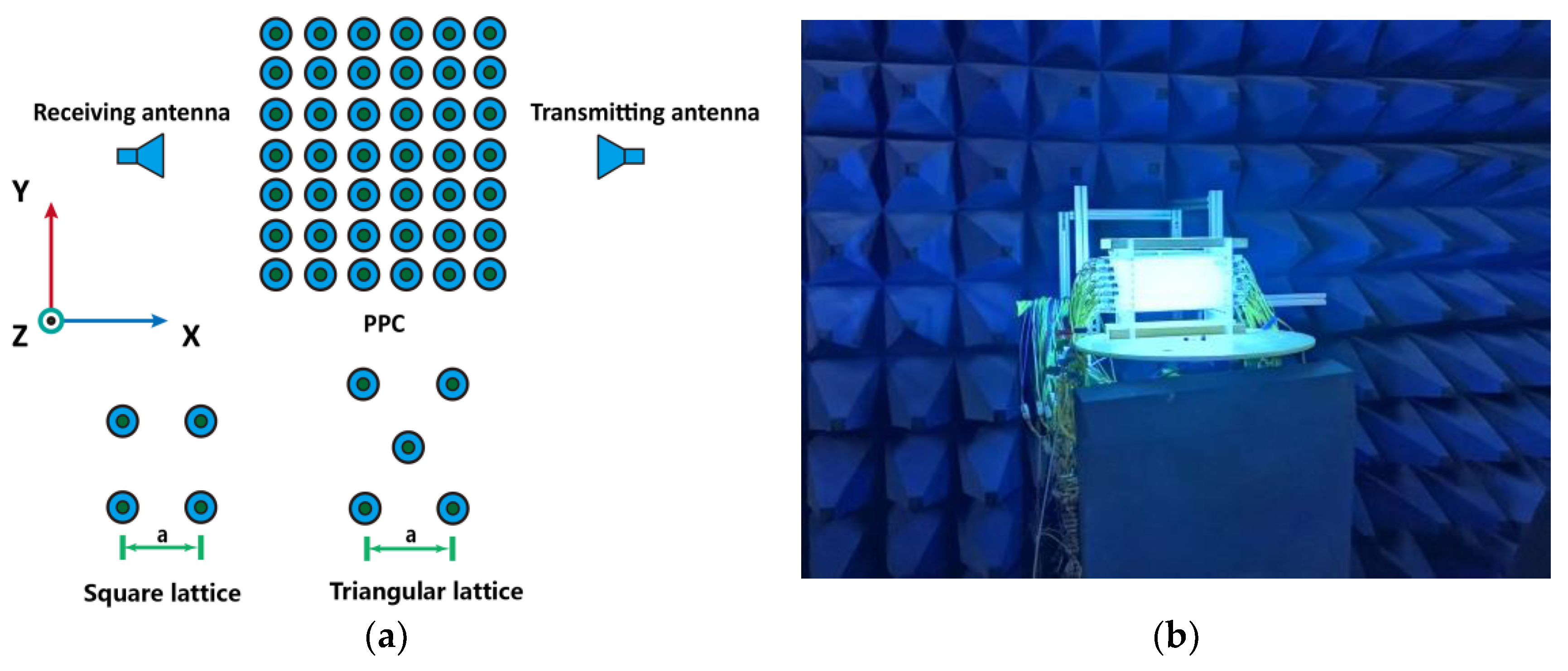
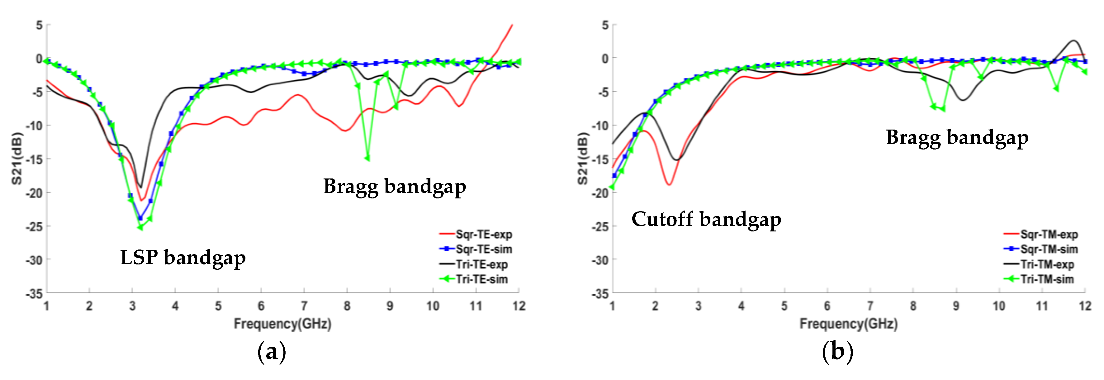
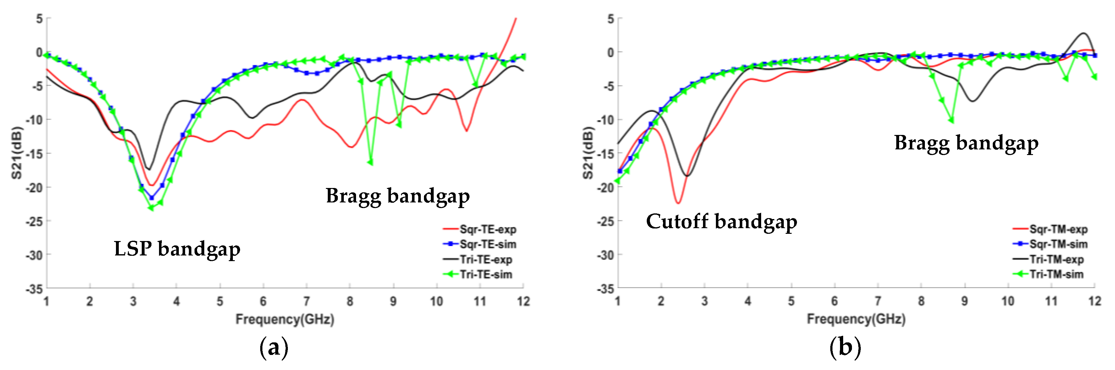
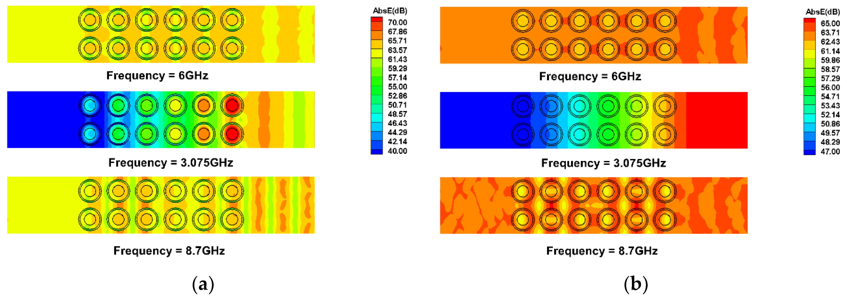
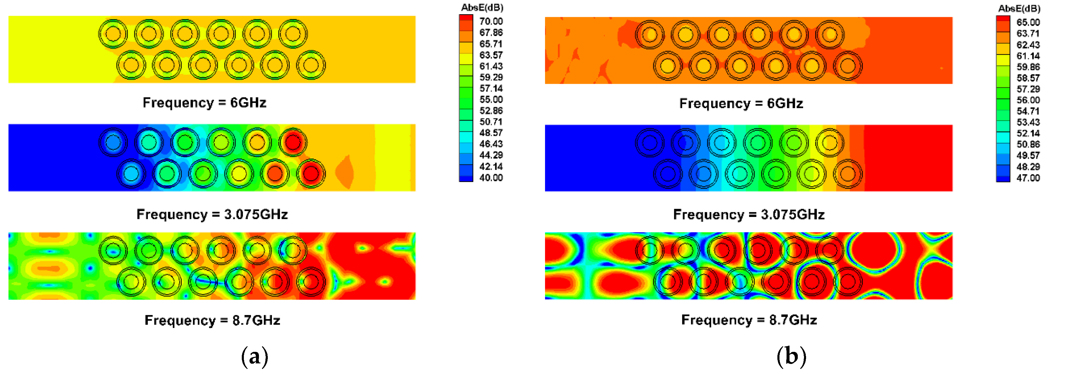
2.2. The Transmission Characteristics of PPC

The calculation and experimental results of the transmission spectra are shown in Figure 4, Figure 5 and Figure 6. In the legend, “Sqr” means square lattice, “Tri” means triangular lattice, “TE−like” means TE−like polarization, “TM−like” means TM−like polarization, “exp” represents the experimental results, and “sim” represents the numerical results.
Figure 4, Figure 5 and Figure 6 show that, under TE−like polarization, a wider and deeper bandgap appears near 3 GHz in each transmission spectra, which may be due to the localized surface plasmon (LSP) generated by the electromagnetic wave on the plasma surface under TE−like polarization, and the depth of the LSP bandgap is much larger than the conventional photonic bandgap generated by Bragg scattering. The main method of electron generation in the discharge tube is the hot electron emission from the cathode. As the discharge current rises, the temperature of the cathode rises, the number of electrons escaping from the cathode increases, the electron density increases, the plasma frequency rises, and the bandgap moves to a higher frequency. Additionally, as the electron density increases, the collision frequency of the plasma in the discharge tube increases. From the Drude model, it can be seen that the collision frequency increases, the imaginary part of the plasma dielectric constant decreases, i.e., the loss of electromagnetic wave propagation in it decreases, so the bandgap depth becomes shallow. When the frequency is greater than 5 GHz, the dielectric constant of the plasma tends to a vacuum, so the value of the transmission spectra is close to 0. The experimental and simulated transmission curves are in good agreement, indicating that the established layered model is reasonable.
It can be deduced from the Maxwell equations in the medium that electromagnetic waves cannot generate LSP on the plasma surface under TM−like polarization [19]. At this point, there is a cutoff region (1 to 3 GHz) in the transmission spectrum, and electromagnetic waves cannot be transmitted in this region due to the cutoff effect of the plasma on electromagnetic waves below the plasma frequency. However, the cutoff frequencies in Figure 4b, Figure 5b and Figure 6b are lower than the plasma frequency, which indicates that the cutoff phenomenon is somewhat weakened when the plasma is used as a scatterer.
Comparing the transmission spectra of triangular and square lattice PPCs, it can be found that, under a TM−like mode, around 8.5 GHz, the triangular lattice PPC has an extra bandgap. The reason may be that the structure of the triangular lattice is more compact, and electromagnetic waves are more prone to generate Bragg scattering. Figure 4, Figure 5 and Figure 6 show that the bandgap of PPCs is determined by the polarization direction and the lattice type.
The difference between the experimental and numerical results may be caused by the following reasons: the length of the plasma tube in the experiment is limited, and the plasma distribution is not uniform, and the plasma distribution near the electrodes is significantly different from the central region of the plasma tube; the calculation considers that the plasma tube is infinitely long and the plasma is considered uniform. The metal sheath at both ends of the plasma tube may have some influence on the results. In addition, due to the limited number of plasma tubes, the PPC cannot cover the antenna completely under TM−like polarization, and the low-frequency electromagnetic waves may enter the receiving antenna due to diffraction, so the experimental and simulated transmission curves differ below 2 GHz.
Figure 7 and Figure 8 show the calculation results of the electric field distribution when the discharge power P1 = 6.28 W. Under TE−like polarization with a frequency of 3.075 GHz (within the bandgap), in the rightmost plasma tube, the electric field is significantly enhanced at the intersection of plasma and air, and this is consistent with the phenomenon generated by LSP [20]. Under TM−like polarization, when the frequency is 1 GHz (within the cutoff bandgap), there is no LSP-like phenomenon in the electric field. When the incident frequency is 8.7 GHz (within the Bragg bandgap), the triangular lattice will have a conventional photonic bandgap under the two polarization modes, while the square lattice has no bandgap. The reason is as mentioned above. The more compact structure of the triangular lattice leads to Bragg scattering in the PPC, but the Bragg bandgap does not cause electromagnetic waves to be absorbed, so the bandgap depth is significantly smaller than the LSP bandgap. Therefore, the cause of the photonic bandgap is closely related to the polarization mode and the lattice structure. At the same time, the change in the lattice structure significantly changes the distribution of the electric field.

2.3. The Bandstructure of PPC

In this section, the bandstructure of the PPC is calculated by SFDTD, PWE, and FEM. Since the variation of electron density only affects the bandgap position, not the bandstructure and bandgap type, so the case of discharge power P1 = 6.28 W (ne1 = 2.64 × 10¹⁷/m3) is chosen for analysis in this section. A comparison of the bandstructure and transmission spectra is shown in Figure 9 and Figure 10.
From Figure 9a–c and Figure 10a–c, it can be seen that the flat band appears in the bandstructure at frequencies of 2 to 4 GHz under TE−like polarization, which corresponds to the bandgap in the transmission spectra. The reason for the generation of the flat band is the presence of LSP, which is a common feature of the bandstructure under TE−like polarization in metallic photonic crystals and plasma photonic crystals.
On bounded surfaces, LSP can be generated by direct irradiation of electromagnetic waves, which is essentially a resonance phenomenon. The incident electric field exerts a force on the free electrons in the plasma, thus causing the free electrons to be deflected relative to the positive ions, and the Coulomb force between the positive ions and the electrons acts as an effective restoring force to pull the driven deflected electrons toward its equilibrium position, thus causing resonance [13].
The LSP has two significant effects: first, the incident wave undergoes strong absorption and scattering at the LSP resonant frequency; second, there is a locally enhanced electric field. Moreover, the LSP generated on the cylindrical PPC can be regarded as a standing wave of the surface plasma wave propagating in the opposite direction, and the electric field distribution with a knot-belly structure at the plasma-air interface can be observed in both Figure 7a and Figure 8a.
A conventional photonic bandgap appears near the frequency of 7 GHz, which arises due to Bragg scattering caused by the periodic variation of the dielectric constant. From the transmission spectra, it can be seen that the depth of the bandgap generated by the LSP is larger than that of the Bragg bandgap. Since LSP is not generated under TM−like polarization, there is no flat band in Figure 9b–d and Figure 10b–d.
Figure 9 and Figure 10 show that the bandstructure results of the three methods are in better agreement with the experiments. Compared with the traditional FDTD method, SFDTD constructs the symplectic scheme by the high-order symplectic integral method, which has better numerical accuracy, but the multi-stage time advance and the high-order spatial difference will increase the computation; the PWE method is simple to program and fast to calculate; however, the generality is poor, and the calculation formula varies with the increase in medium type; an FEM method based on weak form equation simplifies the nonlinear eigenvalue problem into a linear eigenvalue problem, which saves computational effort.
The bandstructure calculated by the SFDTD may “miss” or “misrecord” the eigenfrequencies because the calculation results of SFDTD depend on the number and location of excitation sources and monitors. PWE and FEM methods will calculate some “pseudo” eigenfrequencies when calculating the TE−like polarization bandstructure, because the presence of LSP in PPCs makes it difficult to converge when solving for the complex eigenvalues. Therefore, a combination of the three methods and experimental results is needed to analyze the bandgap type of PPCs comprehensively and accurately.

3. Conclusions

In this paper, the transmission characteristics of triangular and square lattice PPCs with different polarization modes are tested and simulated, the bandstructure of PPCs is calculated by SFDTD, PWE, and FEM methods based on weak form equations, and the bandgap types of PPCs are analyzed. Combining the above results, the following conclusions are obtained.
  • A layered model is established for the plasma discharge tube, the simulation and experiment results of the transmission spectra are in good agreement, indicating that the layered model is reasonable.
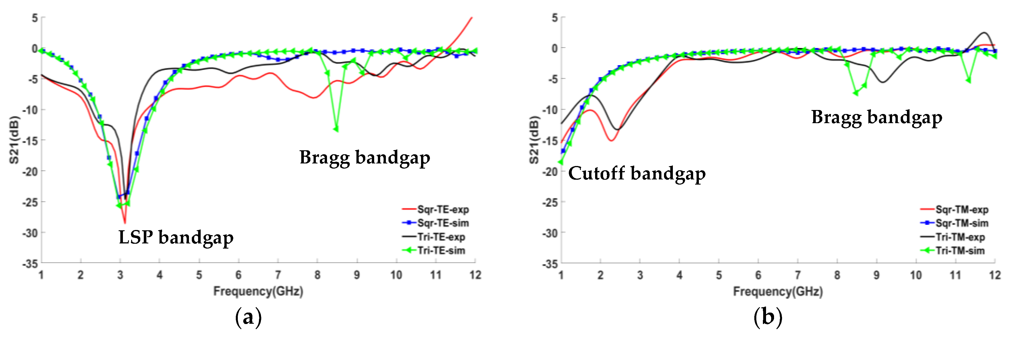
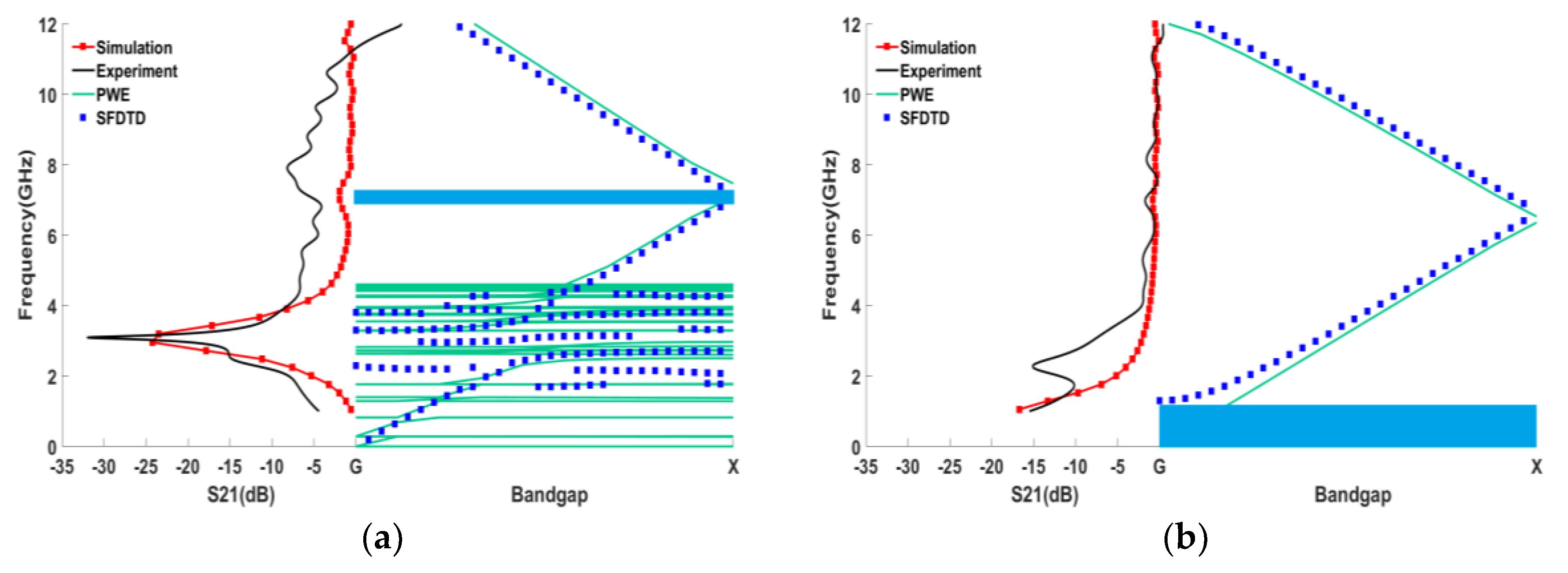
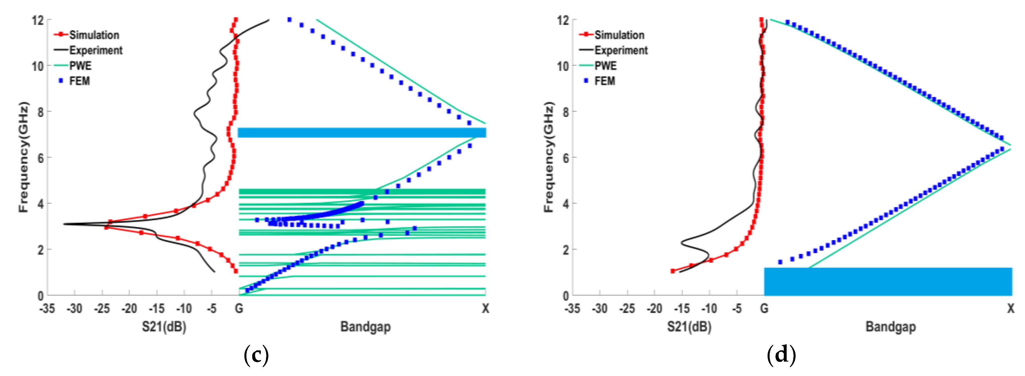
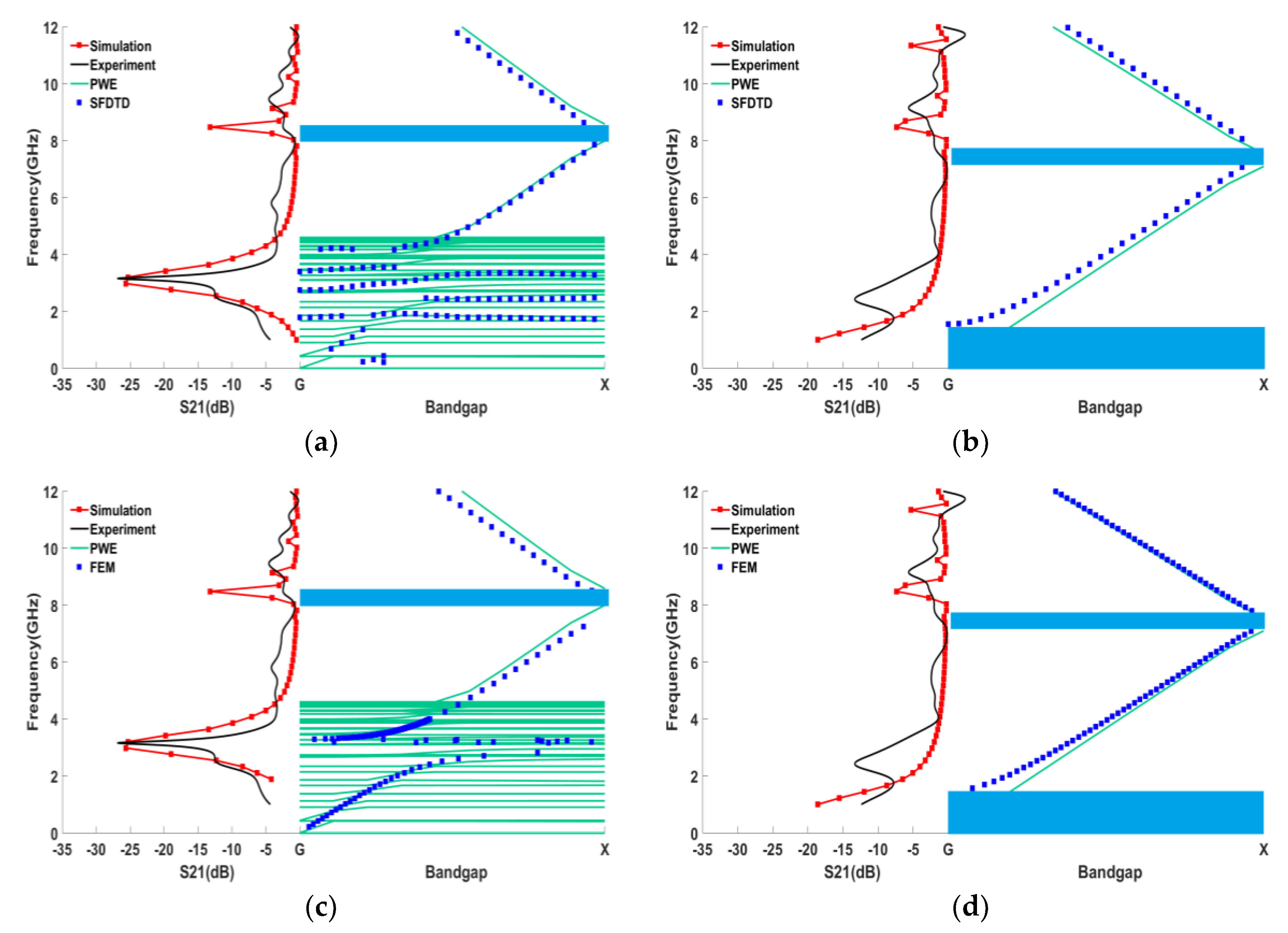
  • The bandgap of a PPC is determined by the polarization direction and lattice type. The rise in electron density and collision frequency makes the LSP bandgap move toward high frequency and the bandgap depth becomes shallow.
  • The type of bandgap in the transmission spectra can be determined by the bandstructure: a flat band in the bandstructure indicates the presence of LSP in the PPC, and regular bandgap is generated by Bragg scattering and the cutoff effect of plasma on electromagnetic waves.
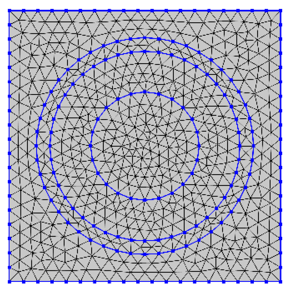
  • SFDTD, PWE, and FEM can calculate bandstructure; each has its advantages and disadvantages. Therefore, it is necessary to combine the results of the three methods and the experimental test results to accurately determine the bandgap type of the PPC.

Author Contributions

Conceptualization, Q.L.; Data curation, Y.L.; Methodology, Y.L.; Resources, Z.L., J.P., L.L. and R.L.; Software, Y.L.; Writing—original draft, Y.L.; Writing—review & editing, Q.L. All authors have read and agreed to the published version of the manuscript.

Funding

National Natural Science Foundation of China (51707169), National Natural Science Foundation of Fujian Province, China (2019J01042), Aeronautical Power Fund Project, China (6141B09050390), Project on the integration of Industry, Education and Research of Aero Engine Corporation of China (HFZL2018CXY009), Fundamental Research Funds for the Central Universities (20720210050).

Conflicts of Interest

The authors declare no conflict of interest.

Appendix A. Modified Plane Wave Expansion Method

In the case of the TE (H polarization) mode, the z component of magnetic field Hz is
H z ( x | ω ) = G A ( k | G ) e j ( k + G ) x
when we substitute Equation (A1) into the wave equation about Hz, coefficients A ( k | G ) fulfill the following equation as
G ( k + G ) ( k + G ) H f ( G G ) A ( k | G ) = ω 2 c 2 A ( k | G )
where H f ( G ) are the Fourier coefficients of 1 / ε ( x | ω ) , and G is a reciprocal-lattice vector.
H f ( G ) = 1 s S ε ( r ) exp ( j G r ) d r
ε ( r ) = 1 ε b + ( 1 ε p 1 ε b ) F 1 ( r ) + ( 1 ε q 1 ε b ) F 2 ( r )
F 1 ( r ) = { 1 ,   i n   t h e   p l a s m a   r e g i o n 0 ,   i n   t h e   t h e   a i r   r e g i o n
F 2 ( r ) = { 1 ,   i n   t h e   q u a r t z   r e g i o n 0 ,   i n   t h e   t h e   a i r   r e g i o n
In order to calculate Fourier coefficients of photonic crystal of arbitrary shape, numerical integration method could be used. Here, takes the square lattice as an example, as Figure A1 shows.
H f ( G ) = 1 s i = 1 M ε ( x i , y i ) exp ( j ( G x x i + G y y i ) ) Δ a i
where subscript i represents the ith element, M is the total number of element, Δai is the area of ith element, ( x i , y i ) is the coordinate of the center of ith element, ε ( x i , y i ) is the value of Equation (A4) in ith element, ( G x , G y ) is the x-component and y-component of G .
Figure A1. Calculating mesh.
Photonics 08 00401 g0a1
Using Equations (A2) and (A7) and μ = ω / c , Equation (A2) yields
μ 4 I μ 3 X 3 μ 2 X 2 μ X 1 X 0 = 0
where
X 3 ( G | G ) = j v c δ G , G
X 2 ( G | G ) = 1 s i = 1 M ε q + F 2 ε b F 1 ε q F 2 ε q + F 1 ε b ε q ε b ε q exp { j [ ( G x G x ) x i + ( G y G y ) y i ] } Δ a i ( k + G ) ( k + G ) + ω p 2 c 2 δ G G
X 1 ( G | G ) = 1 s i = 1 M ε q + F 2 ε b F 1 ε q F 2 ε q + F 1 ε b ε q ε b ε q exp { j [ ( G x G x ) x i + ( G y G y ) y i ] } Δ a i ( k + G ) ( k + G ) j v c
X 0 ( G | G ) = 1 s i = 1 M ε q + F 2 ε b F 1 ε q F 2 ε q ε b ε q exp { j [ ( G x G x ) x i + ( G y G y ) y i ] } Δ a i ( k + G ) ( k + G ) ( ω p 2 c 2 )
where the elements of the N × N matrices are X3 X2 X1 X0. N is the number of plane wave. This polynomial form is transformed into a linear problem in 4N dimensions by W that fulfills
W z = μ z , W = [ O       I       O       O O       O       I       O O       O       O       I X 0 X 1 X 2 X 3 ]
Similarly, for the TM (E polarization) mode, the calculation formula is directly given here:
μ 3 X 3 μ 2 X 2 μ X 1 X 0 = 0
X 3 ( G | G ) = 1 s i = 1 M ( F 1 + ε b F 1 ε b F 2 ε b + F 2 ε q ) exp { j [ ( G x G x ) x i + ( G y G y ) y i ] } Δ a i
X 2 ( G | G ) = X 3 ( G | G ) ( j v c )
X 1 ( G | G ) = 1 s i = 1 M ( F 1 ω p 2 c 2 ) exp { j [ ( G x G x ) x i + ( G y G y ) y i ] } Δ a i ( k + G ) 2 δ G G
X 0 ( G | G ) = j v c ( k + G ) 2 δ G G
where the elements of N × N matrices are X3 X2 X1 X0. This polynomial form is transformed into a linear problem in 3N dimensions by Q and V that fulfills
Q z = μ V z , Q = [ O       I       O O       O       I X 0 X 1 X 2 ] , V = [ I       O       O O       I       O O       O     X 3 ]

Appendix B. Derivation of Weak Form Equations

Taking the TE mode as an example, the Maxwell equation is:
× ( 1 ε × H ) μ ω 2 c 2 H = 0
According to Bloch′s theorem, the magnetic field H can be expanded as:
H ( x ) = u ( x ) exp [ i ( ω t k x ) ]
Substituting Equation (A21) into Equation (A20), Equation (A20) can be obtained:
k 2 ε u k ε ( k u ) i k × ( 1 ε ) i × ( 1 ε k × u ) + × ( 1 ε × u ) μ ω 2 c 2 u = 0
Both sides of Equation (A22) are multiplied by the weight function v
F H ( v , u ) = k 2 ε v u k ε ( k v ) ( k u ) i ( 1 ε ) v [ k × ( × u ) ] i ( × v ) 1 ε ( k × u ) + ( × v ) 1 ε ( × u ) μ ω 2 c 2 v u
The FEM method requires the integration over the computational region provided that the equations and boundary conditions are satisfied, and let Equation (A23) equal zero:
0 = Ω d 3 x F H ( v , u ) = Ω d 3 x   v [ 1 ε k × ( k × u ) i 1 ε v k × ( × u ) + × ( 1 ε × u ) μ ω 2 c 2 u ] + Ω d A v [ n × 1 ε ( i k × u + × u ) ]
For a 2D problem, Equation (A24) can be simplified to:
F H z ( H ~ z , H z ) = d 2 x [ × H ~ z 1 ε × H z H ~ z μ ω 2 c 2 H z ]
With the following substitutions H z = h z e i k x , H ~ z = h ~ z e i k x , where H z ~ is weight function, Equation (A25) becomes Equation (B7):
F H z ( H ~ z , H z ) = d 2 x [ ( i k + ) h ~ z 1 ε ( i k + ) h z h ~ z μ ω 2 c 2 h z ]
where k = k 0 + λ k n .
The contents of the square brackets in Equation (A26) are entered according to the COMSOL format, and λ is the eigenvalue to be determined.
Similarly, the weak form equation of TM mode is Equation (A27):
F E z ( E z ~ , E z ) = d 2 x [ ( i k + ) × E z ~ 1 μ ( i k + ) × E z E z ~ ε ω 2 c 2 E z ]

Appendix C. The Scheme of SFDTD

In this paper, we use the SFDTD (5, 4) scheme, which means five steps advance in the time direction and a fourth order difference in the space direction. The iteration scheme of SFDTD is:
H n + l / m = H n + ( l 1 ) / m c l Δ t μ 0 ( × E n + ( l 1 ) / m )
J n + l / m = ( 2 v c l Δ t 2 + v c l Δ t ) J n + ( l 1 ) / m + 2 ε 0 c l ω p 2 Δ t ( 2 + v c l Δ t ) E n + ( l 1 ) / m
E n + l / m = E n + ( l 1 ) / m + d l Δ t ε 0 [ ( × H n + l / m ) J n + l / m ]
where l = 0, 1, 2…5, m = 5, cl and dl are symplectic propagator. The specific coefficients are in [21,22].

References

  1. Sakai, O.; Sakaguchi, T.; Tachibana, K. Verification of a plasma photonic crystal for microwaves of millimeter wavelength range using two-dimensional array of columnar microplasmas. Appl. Phys. Lett. 2005, 87, 241505. [Google Scholar] [CrossRef] [Green Version]
  2. Sakai, O.; Sakaguchi, T.; Ito, Y.; Tachibana, K. Interaction and control of millimetre-waves with microplasma arrays. Plasma Phys. Control. Fusion 2005, 47, B617–B627. [Google Scholar] [CrossRef]
  3. Fan, W.; Zhang, X.; Dong, L. Two-dimensional plasma photonic crystals in dielectric barrier discharge. Phys. Plasmas 2010, 17, 113501. [Google Scholar] [CrossRef]
  4. Wang, Y.; Dong, L.; Liu, W.; He, Y.; Li, Y. Generation of tunable plasma photonic crystals in meshed dielectric barrier discharge. Phys. Plasmas 2014, 21, 73505. [Google Scholar] [CrossRef]
  5. Wang, B.; Guez, J.A.R.I.; Cappelli, M.A. 3D woodpile structure tunable plasma photonic crystal. Plasma Sources Sci. Technol. 2019, 28, 02LT01. [Google Scholar] [CrossRef] [Green Version]
  6. Zhang, L.; Ouyang, J. Experiment and simulation on one-dimensional plasma photonic crystals. Phys. Plasmas 2014, 21, 103514. [Google Scholar] [CrossRef]
  7. Wen, Y.; Liu, S.; Zhang, H.; Wang, L. The absorber realized by 2D photonic crystals with plasma constituents. J. Phys. D Appl. Phys. 2018, 51, 25108. [Google Scholar] [CrossRef]
  8. Wang, B.; Cappelli, M.A. A plasma photonic crystal bandgap device. Appl. Phys. Lett. 2016, 108, 161101. [Google Scholar] [CrossRef]
  9. Arkhipenko, V.I.; Callegari, T.; Simonchik, L.V.; Sokoloff, J.; Usachonak, M.S. One-dimensional electromagnetic band gap structures formed by discharge plasmas in a waveguide. J. Appl. Phys. 2014, 116, 123302. [Google Scholar] [CrossRef]
  10. Babitski, V.S.; Callegari, T.; Simonchik, L.V.; Sokoloff, J.; Usachonak, M.S. One-dimensional electromagnetic band gap plasma structure formed by atmospheric pressure plasma inhomogeneities. J. Appl. Phys. 2017, 122, 83302. [Google Scholar] [CrossRef]
  11. Iwai, A.; Righetti, F.; Wang, B.; Sakai, O.; Cappelli, M.A. A tunable double negative device consisting of a plasma array and a negative-permeability metamaterial. Phys. Plasmas 2020, 27, 23511. [Google Scholar] [CrossRef]
  12. Wang, B.; Rodríguez, J.A.; Miller, O.; Cappelli, M.A. Reconfigurable plasma-dielectric hybrid photonic crystal as a platform for electromagnetic wave manipulation and computing. Phys. Plasmas 2021, 28, 43502. [Google Scholar] [CrossRef]
  13. Righetti, F.; Wang, B.; Cappelli, M.A. Enhanced attenuation due to lattice resonances in a two-dimensional plasma photonic crystal. Phys. Plasmas 2018, 25, 124502. [Google Scholar] [CrossRef]
  14. Tan, H.; Jin, C.; Zhuge, L.; Wu, X. Simulation on the Photonic Bandgap of 1-D Plasma Photonic Crystals. IEEE Trans. Plasma Sci. 2018, 46, 539–544. [Google Scholar] [CrossRef]
  15. Zhang, Y.; Wen, X.; Yang, W. Excitation temperatures of atmospheric argon in dielectric barrier discharges. Plasma Sources Sci. Technol. 2007, 16, 441–447. [Google Scholar] [CrossRef]
  16. Walker, A.L.; Curry, D.L.; Fannin, H.B. Comparison of Methodologies for the Determination of Excitation Temperatures of Plasma Support Gases. Appl. Spectrosc. 1994, 48, 333–337. [Google Scholar] [CrossRef]
  17. NIST: Atomic Spectra Database Lines Form. Available online: https://physics.nist.gov/PhysRefData/ASD/lines_form.html (accessed on 6 August 2021).
  18. Hagelaar, G.J.M.; Pitchford, L.C. Solving the Boltzmann equation to obtain electron transport coefficients and rate coefficients for fluid models. Plasma Sources Sci. Technol. 2005, 14, 722–733. [Google Scholar] [CrossRef]
  19. Maier, S.A. Plasmonics: Fundamentals and Applications; Springer: Berlin/Heidelberg, Germany, 2007. [Google Scholar]
  20. Ito, T.; Sakoda, K. Photonic bands of metallic systems. II. Features of surface plasmon polaritons. Phys. Rev. B 2001, 64, 1–8. [Google Scholar] [CrossRef]
  21. Hermansson, B.; Yevick, D. Generalized propagation techniques-application to semiconductor rib waveguide Y-junctions. IEEE Photonics Technol. Lett. 1990, 2, 738–740. [Google Scholar] [CrossRef]
  22. He, Z.; Liu, S.; Chen, S.; Zhong, S. Application of symplectic finite-difference time-domain scheme for anisotropic magnetised plasma. IET Microw. Antennas Propag. 2017, 11, 600–606. [Google Scholar] [CrossRef]
Figure 1. (a) Schematic diagram of PPC lattice. (b) Experiment photo.
Photonics 08 00401 g001
Figure 2. (a) Discharge tube model and location of measuring points. (b) PPC model of calculation.
Photonics 08 00401 g002
Figure 3. Electron excitation temperature distribution of discharge tube. (a) Changes in electron excitation temperature at each measuring point with power. (b) Distribution of electron excitation temperature along the axis under different powers.
Photonics 08 00401 g003
Figure 4. Discharge power P1 = 6.28 W, ne1 = 2.64 × 10¹⁷/m3, transmission spectra of PPC: (a) TE−like polarization; (b) TM−like polarization.
Photonics 08 00401 g004
Figure 5. Discharge power P2 = 6.43 W, ne2 = 2.92 × 10¹⁷/m3, transmission spectra of PPC: (a) TE−like polarization; (b) TM−like polarization.
Photonics 08 00401 g005
Figure 6. Discharge power P3 = 6.56 W, ne3 = 3.36 × 10¹⁷/m3, transmission spectra of PPC: (a) TE−like polarization; (b) TM−like polarization.
Photonics 08 00401 g006
Figure 7. Electric field distribution of square lattice PPC at different frequencies: (a) TE−like polarization; (b) TM−like polarization.
Photonics 08 00401 g007
Figure 8. Electric field distribution of triangular lattice PPC at different frequencies: (a) TE−like polarization; (b) TM−like polarization.
Photonics 08 00401 g008
Figure 9. Square lattice PPC, comparison of bandstructure and transmission spectra: (a) TE−like polarization, bandstructure calculated by SFDTD and PWE; (b) TM−like polarization, bandstructure calculated by SFDTD and PWE; (c) TE−like polarization, bandstructure calculated by FEM and PWE; (d) TM−like polarization, bandstructure calculated by PWE and FEM.
Photonics 08 00401 g009aPhotonics 08 00401 g009b
Figure 10. Triangular lattice PPC, comparison of bandstructure and transmission spectra: (a) TE−like polarization, bandstructure calculated by SFDTD and PWE; (b) TM−like polarization, bandstructure calculated by SFDTD and PWE; (c) TE−like polarization, bandstructure calculated by FEM and PWE; (d) TM−like polarization, bandstructure calculated by PWE and FEM.
Photonics 08 00401 g010
Table 1. Spectroscopic data corresponding to the selected Hg I emission spectrum.
λ i j (nm) A i j (10−7s−1) ε i (eV) g i
253.65210.844.8873
312.65746.68.8525
365.015812.908.8577
404.65652.077.7313
435.83355.607.7313
546.0754.97.7315
Publisher’s Note: MDPI stays neutral with regard to jurisdictional claims in published maps and institutional affiliations.

