Article

SP-ILC: Concurrent Single-Pixel Imaging, Object Location, and Classification by Deep Learning

1
State Key Laboratory of Low-Dimensional Quantum Physics and Department of Physics, Tsinghua University, Beijing 100084, China
2
Wuhan Digital Engineering Institute, Wuhan 430074, China
3
Frontier Science Center for Quantum Information, Beijing 100084, China
*
Author to whom correspondence should be addressed.
Photonics 2021, 8(9), 400; https://doi.org/10.3390/photonics8090400
Submission received: 6 August 2021 / Revised: 14 September 2021 / Accepted: 15 September 2021 / Published: 18 September 2021
(This article belongs to the Special Issue Smart Pixels and Imaging)

Abstract

:
We propose a concurrent single-pixel imaging, object location, and classification scheme based on deep learning (SP-ILC). We used multitask learning, developed a new loss function, and created a dataset suitable for this project. The dataset consists of scenes that contain different numbers of possibly overlapping objects of various sizes. The results we obtained show that SP-ILC runs concurrent processes to locate objects in a scene with a high degree of precision in order to produce high quality single-pixel images of the objects, and to accurately classify objects, all with a low sampling rate. SP-ILC has potential for effective use in remote sensing, medical diagnosis and treatment, security, and autonomous vehicle control.

1. Introduction

Single-pixel imaging (SPI) uses a single pixel detector instead of an array detector to obtain information about an object. The random patterns or orthogonal patterns such as Fourier transform basis patterns and Hadamard transform basis patterns are used to encode the light field illuminating on the object and the reflected light is collected by a single-pixel detector [1,2]. Single-pixel detectors can operate in spectral bands, such as THz, infrared and X-ray bands [3,4,5], that are not accessible to array detectors because of cost or technical constraints. Single-pixel imaging and the related technique of computational ghost imaging have recently attracted widespread attention [6,7,8,9,10,11,12,13]. Single-pixel imaging has important applications in 3D imaging [14,15], LiDAR [16], encrypted communication [17], and many other fields.
Deep learning has powerful feature extraction capabilities [18,19]. Many advances in deep learning have been made recently in, for example, image classification [20], object detection [21], and image segmentation [22,23,24]. Deep learning has been found to improve the quality of single-pixel imaging and to reduce the impact of noise on imaging; it has also been used for single-pixel object classification [25,26,27,28,29,30,31,32].
Lyu et al. [33] proposed a method of computational ghost imaging based on machine learning in 2017; they were able to recreate high quality images at low sampling rates. Jiao [34] used the S-vector of a single-pixel camera for object classification without the use of images for training or classification in 2018. In addition, in 2018, Higham et al. [35] used deep learning for single-pixel imaging at a frequency that enabled the detection of video images. An important insight in their work was that the speckle pattern used in single-pixel imaging can be treated as a layer of the deep neural network; that is, the speckle pattern can be incorporated into the training process to create an end-to-end system. Wang et al. [36] proposed a method of using simulated data for neural network training in 2019. The training of deep neural networks requires a lot of data, and it is often time-consuming to obtain training data for experiments. The method used by Wang et al. greatly improved the efficiency of neural network training. Zhang et al. [37] developed a method of classifying moving objects using deep learning in 2020.
Great progress has been made in single-pixel imaging and single-pixel classification by combining deep learning [38,39,40]. Studies of single-pixel classification have focused on scenes that contain only a single object, with objects in different scenes being similar in size. However, in practice, the number and size of objects in a scene will vary and objects may overlap [41,42,43,44], which raises a fundamental question: Can a single-pixel imaging system correctly locate and classify multiple objects in a scene? We think it can. Although single-pixel imaging and classification are now treated as separate activities, an end-to-end unified scheme has many benefits; for example, a multitask learning based deep neural network can internally share feature maps between different tasks, thus reducing computer time needed for training, make the network more compact, and increase generalizability.
We propose a single-pixel concurrent imaging, object location, and classification scheme using deep learning. Experiments have shown that SP-ILC can concurrently image, locate and classify different numbers of objects of different sizes that overlap. We used multitask learning based on feature multiplexing techniques, constructed a new loss function, and created a test dataset suitable for this project. We have succeeded in concurrently producing high quality single-pixel images, precisely locating objects, and classifying objects with great accuracy at a low sampling rate. SP-ILC may benefit a wide range of applications such as remote sensing and detection, medical treatments, security, and autonomous vehicle control.
SP-ILC offers the following contributions:
  • SP-ILC is the first image recognition system (to the best of our knowledge) to accurately locate and classify individual or multiple different-sized objects in a scene, even when objects overlap, using a single-pixel camera. Current state-of-the-art single-pixel classification systems with deep learning are able to identify and classify only a single object in a scene;
  • SP-ILC is an end-to-end system based on multitask learning that concurrently detects images, locates objects, and classifies objects in a single process. In contrast to techniques that detect images and identify objects in separate processes, SP-ILC has a compact structure, uses shared feature maps, and has increased generalizability;
  • We have made the code and dataset associated with this study available to other researchers as open source [45].

2. Methods

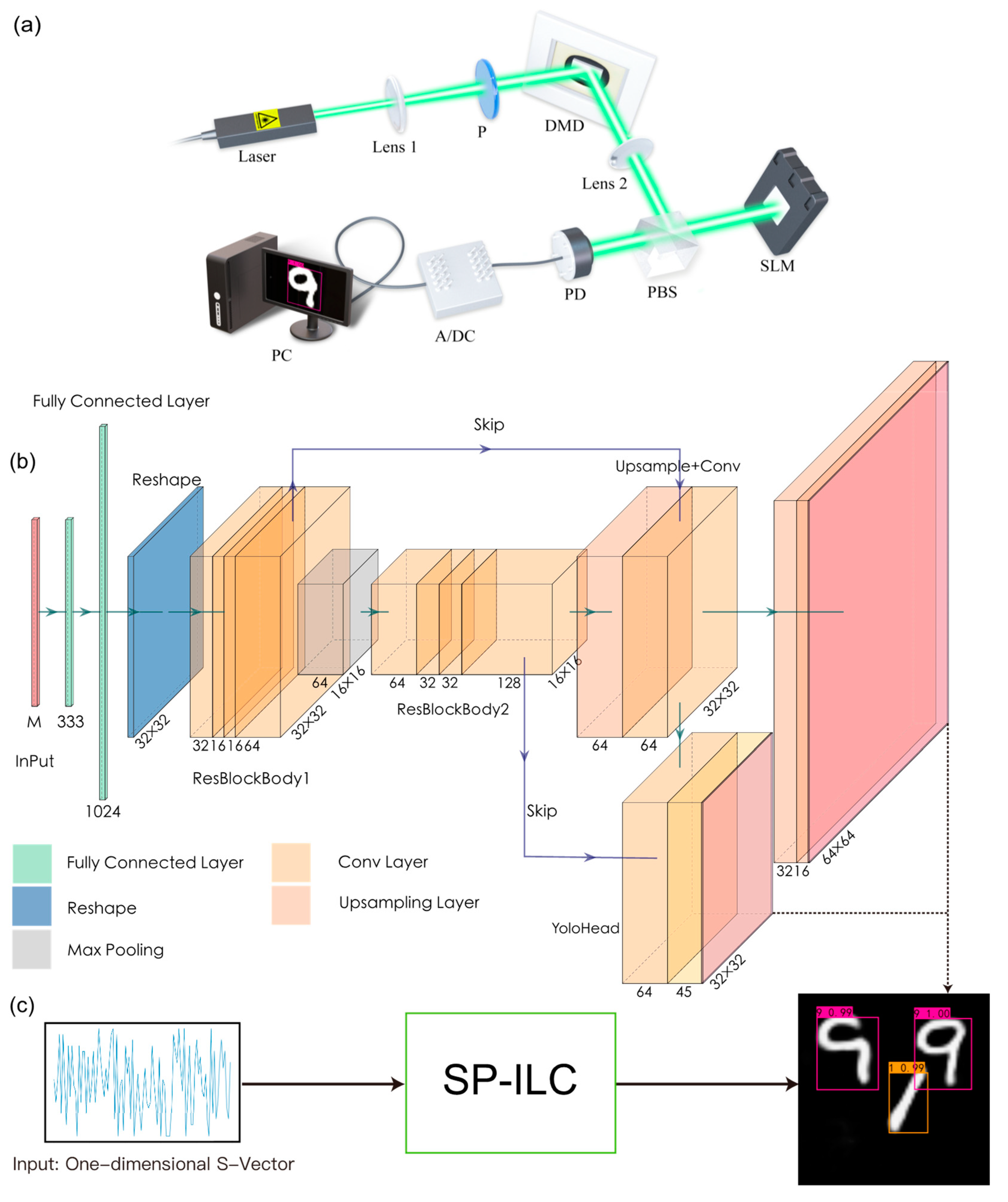
2.1. Experimental Setup and Structure of the Deep Neural Network

The experimental configuration is shown in Figure 1a. This is a typically SPI geometry. The 532 nm laser (F-IVB-500, Yu Guang Co. Ltd.) beam is expanded by lens 1 and illuminates a digital micromirror device (DMD, DLP7000, Texas Instruments) with an operating frequency of 20 kHz to produce a speckle pattern. The speckle patterns are coded by M random matrices consisting only of values 1 or −1 that are determined by the difference between two consecutive DMD patterns; this method also reduces noise [35]. If the kth pattern is denoted by I k ( x , y )   ( k = 1 , 2 , M ) , where x, y are spatial coordinates. The two corresponding DMD patterns are I ˜ k ( x , y )   = [ I k ( x , y ) + 1 ] / 2 and I ˜ k ( x , y )   I k ( x , y ) , respectively [46]. Therefore, M patterns are implemented by 2M DMD frames. The object is displayed by the liquid crystal spatial light modulator (SLM, FSLM-HD70-AP, CAS Microstar), and Lens 2 projects the speckle pattern onto the object. The reflected light passing through the object is received by the bucket detector (DET36A, Thorlab). The light signal detected by the bucket detector undergoes analog-to-digital (A/DC, ADC11C125, Texas Instruments) conversion to produce the bucket signal S k which is defined by:
S k = x , y N I k ( x , y ) × O ( x , y ) ,
where O(x, y) is the object, the size of which is 64 × 64 pixels. After all measurements end, the obtained bucket signal can be seen a one-dimensional vector [ S 1 , , S k , S M ] named S-vector in the following of this paper. S-vector is input to the neural network for imaging, object location, and classification.
The multitask learning deep neural network we used is shown in Figure 1b. The input for training the network is the S-vector of length M and its corresponding label. The S-vector passes through two fully connected layers and is then reshaped to the feature map with a size of 32 × 32 pixels. In addition, this feature map is extracted through the backbone network, which consists of a set of convolutions and two Resblocks. The location and classification tasks are carried out in the backbone network, and a branch from the backbone network is used for the imaging task. The prediction results of the three tasks are summed together to calculate the loss function, and then back-propagated to optimize the parameters. After multiple epochs of training, the final network parameters are determined. The detailed structure of deep neural network of SP-ILC can be found in [45].
In the testing stage, the picture of the test set is displayed on the SLM as the object, and the DMD projects different patterns interacting with the object, and the S-vector is obtained through the single-pixel bucket detector. Next, as shown in Figure 1c, the S-vector obtained through the experiment is sent to the well-trained deep neural network, and SP-ILC will image, locate and classify objects from the one-dimensional S-vector obtained through the experiment concurrently.

2.2. Loss Function

The loss function L that we created consists of three variables:
L = λ 1 L 1 + λ 2 L 2 + λ 3 L 3 ,
where λ t (t = 1, 2, and 3) are hyper-parameters to balance the weight of different tasks. The value of three λ t L t are made to the same level by adjusting the value of λ t to ensure the deep neural network will pay similar attention to the three tasks. The adjusting process to obtain the optimal hyper-parameters by pre-experiment is described in following Section 2.5.
L 1 is the loss function of the image quality evaluation task using root mean square error (RMSE):
L 1 = 1 W × H i = 1 W × H ( G i G ^ i ) 2 ,
where W and H are the width and height of the picture in pixels, both 64. The original picture label and the picture predicted by the deep neural network are represented respectively by G and G ^ . In the remainder of this paper, we use the hat notation to distinguish network prediction results from labels.
L 2 is the loss function for the image location task:
L 2 = i = 0 R 2 j = 0 B l i j obj [ ( x i x ^ i ) 2 + ( y i y ^ i ) 2 ]     + i = 0 R 2 j = 0 B l i j obj [ ( w i w ^ i ) 2 + ( h i h ^ i ) 2 ] .
The first summation in Equation (4) quantifies the distance of the object from the center of the prediction box, and the second summation quantifies the differences in width and height between the prediction box and the true location. The variables x and y are the coordinates of the center of the object, and w and h are the width and height of the object measured through the center of the frame; R is the number of grids the picture is divided into; B is the number of objects that are to be predicted in each grid; and l i j obj is 1 when the object is in grid i and 0 when the object is not in grid i.
L 3 is the loss function for the image classification task:
L 3 = i = 0 R 2 j = 0 B l i j obj ( C i C ^ i ) 2 + λ noobj   i = 0 R 2 j = 0 B l i j noobj   ( C i C ^ i ) 2 + i = 0 S 2 l i obj c     classes   ( p i ( c ) p ^ i ( c ) ) 2 .
The first two summations in Equation (5) quantify the deviation of the prediction classification confidence with respect to two types of inaccurate prediction: the prediction box contains an object but there is no such object in that location on the original image; or the prediction box does not contain an object but there is an object in that location on the original image. C = 1 means there is an object, C = 0 means there is no object, and λ noobj is the weight. The third summation quantifies the difference between the predicted classification and the actual classification; p i ( c ) is the probability that the object belongs to the class c . The forms of Equations (4) and (5) are based on the YOLO loss function in the target detection field [43,44].

2.3. Dataset

The MNIST dataset is commonly used in deep learning [48]. However, each picture in the dataset contains only a single numeric character, there are no position coordinates, and all the number images are approximately the same size. Thus, the MNIST dataset was unsuitable for our experiment. We created a new dataset to be able to detect, locate and classify images of multiple, different-sized, possibly overlapping objects in different positions. We zoomed in or zoomed out on the 28 × 28 pixel images of single numeric characters, and placed them randomly on a 64 × 64 pixel background. Number images may therefore overlap. The training set we produced contains >180,000 pictures. Each picture was multiplied by an M × 4096 random matrix A to obtain the M × 1 S-vector. The 64 × 64 patterns are obtained by resizing each row of matrix A to display on the DMD.
Each S-vector is associated with a three-part label consisting of the original image (used to train the imaging task), location coordinates (used to train the location task), and the image category (used to train the classification task). We developed a labeling program. Each picture in the MNIST dataset contains an image of only one number, so we obtained the bounding box of the single number in the original image by scanning the pixels one by one from the outside to the inside. The bounding box of the single number was mapped onto a bounding box in the final picture, according to the ratio in the resize operation and the number’s location in the final image. The label of the number (in the original dataset) was also used to construct the ground-truth of the final picture.

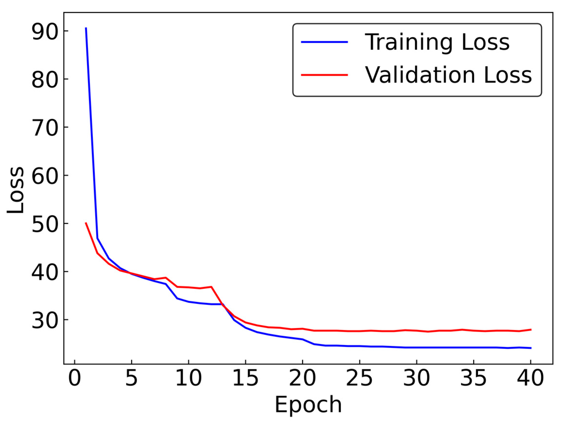
2.4. Training Parameters

The experiments were all conducted on a GeForce RTX 2060 GPU, using the Pytorch framework [49]. The network parameters were all initialized to default values and were updated using SGD with Adam optimization [50]. We trained the model for 40 epochs, with 810 iterations per epoch. We initialize the first fully connected layer of the network as an identity transformation and initialize the rest at random. We divide the 40 epochs into two parts, each of which sets the initial learning rate to be 0.01 and decreases the learning rate by a factor of 0.1 every 8 epochs. The former part contains 12 epochs, in which the first fully connected layer is frozen. The latter contains 28 epochs with all networks unfrozen.

2.5. Other Activities

In this section, we describe how to set the hyperparameters and how to avoid overfitting.
Before we used the dataset of 180k computer-generated data for training, we created an 18k dataset for the pre-experiment. In the pre-experiment, we varied different hyperparameters, such as the initial learning rate, the rate of learning rate decay, and λ in loss function. After several runs of tests, we finally selected the values mentioned in the article.
Overfitting is a very significant concern in machine learning. We paid great attention to it during training and adopted an effective method to avoid it. We set the ratio of the number of computer-generated images in the training set to the number of images in the validation set to be 9:1 and tracked the performance of the loss function of each task using these two datasets during training. We would terminate training and recorded the value of the weights before overfitting occurred if we observed that that training loss has decreased in multiple consecutive epochs but the validation loss has increased during training.
Figure 2 shows a typical training process with the loss decrease and each epoch takes about 20 min.

3. Experimental Results and Analysis

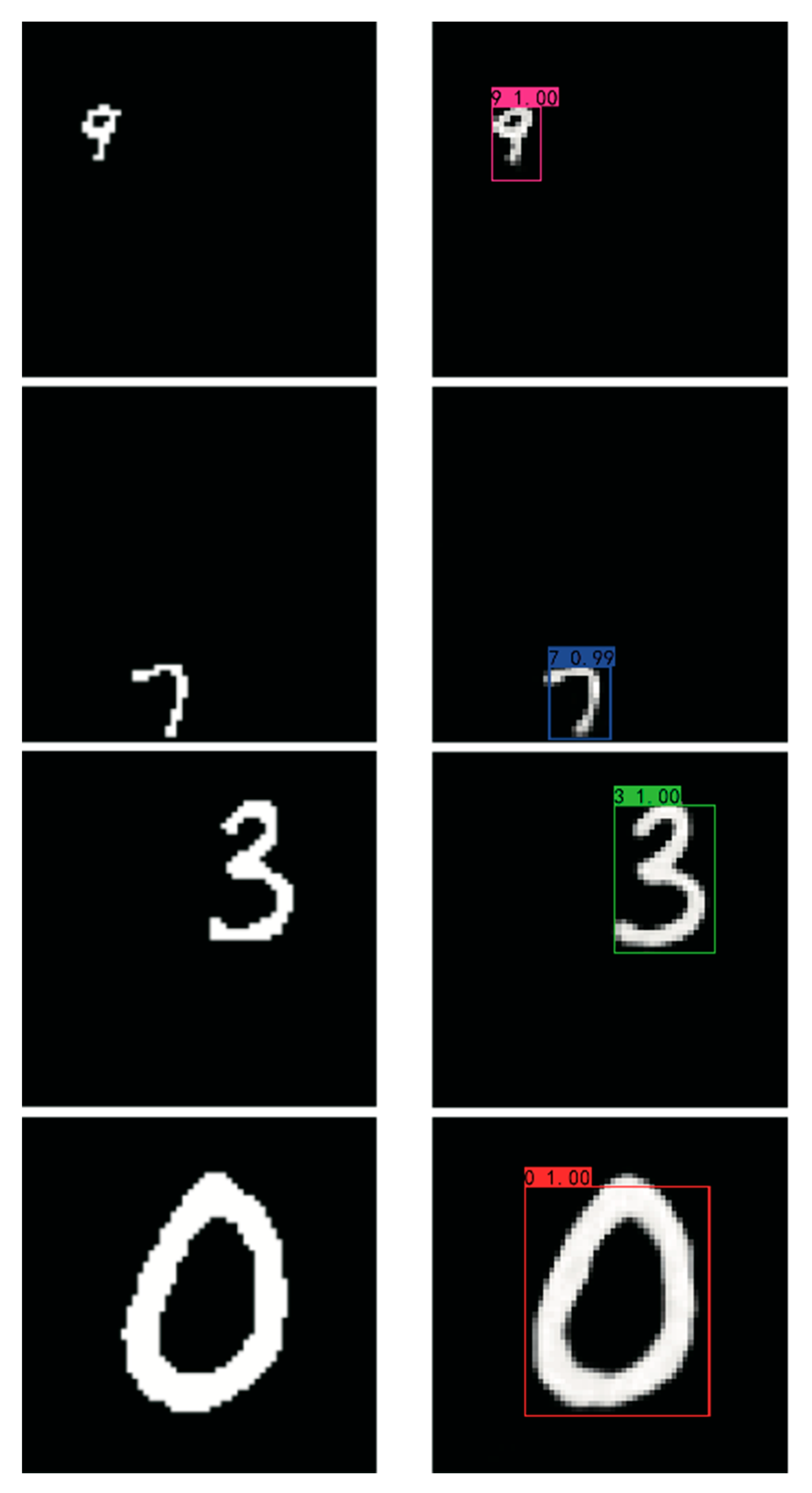
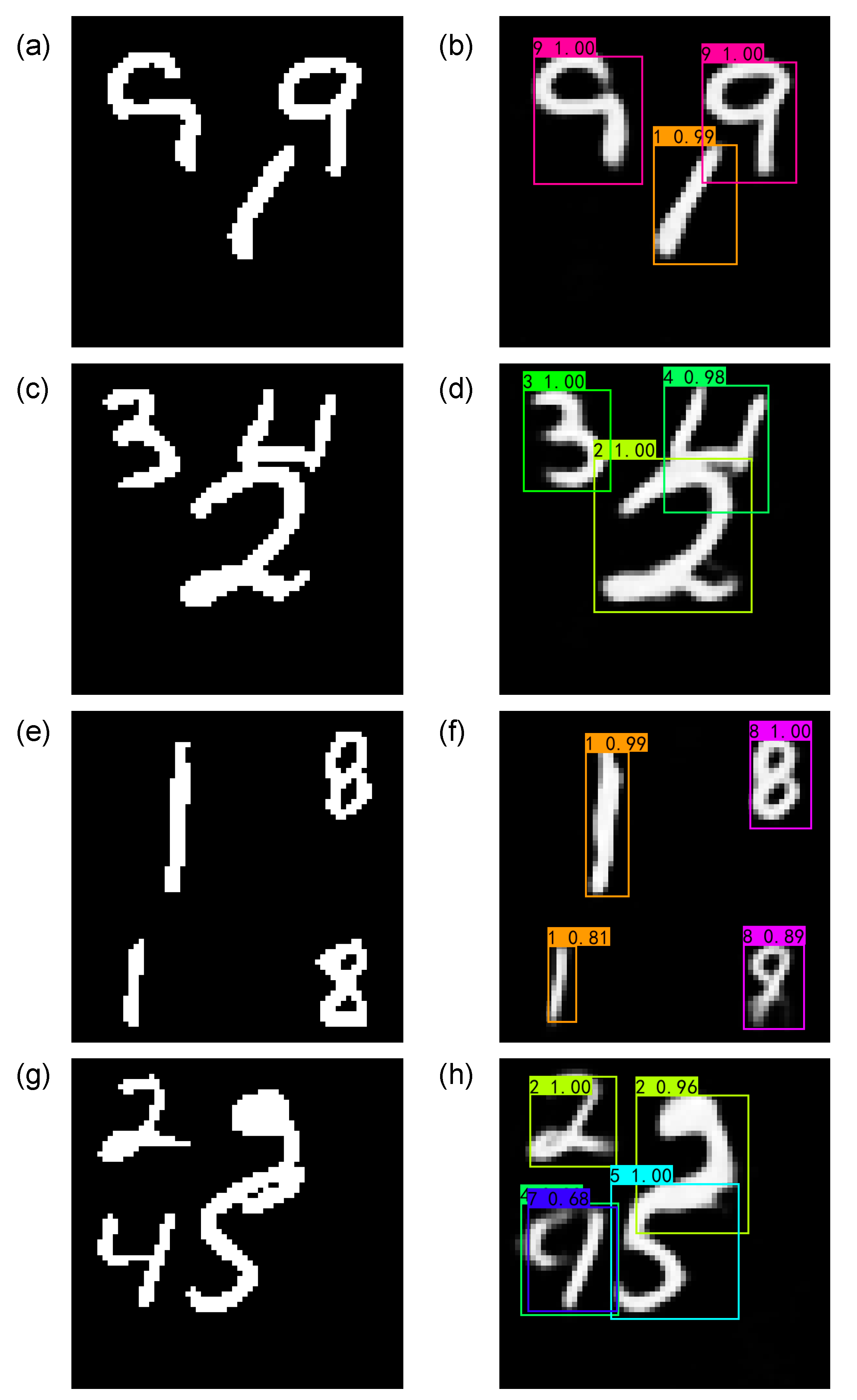
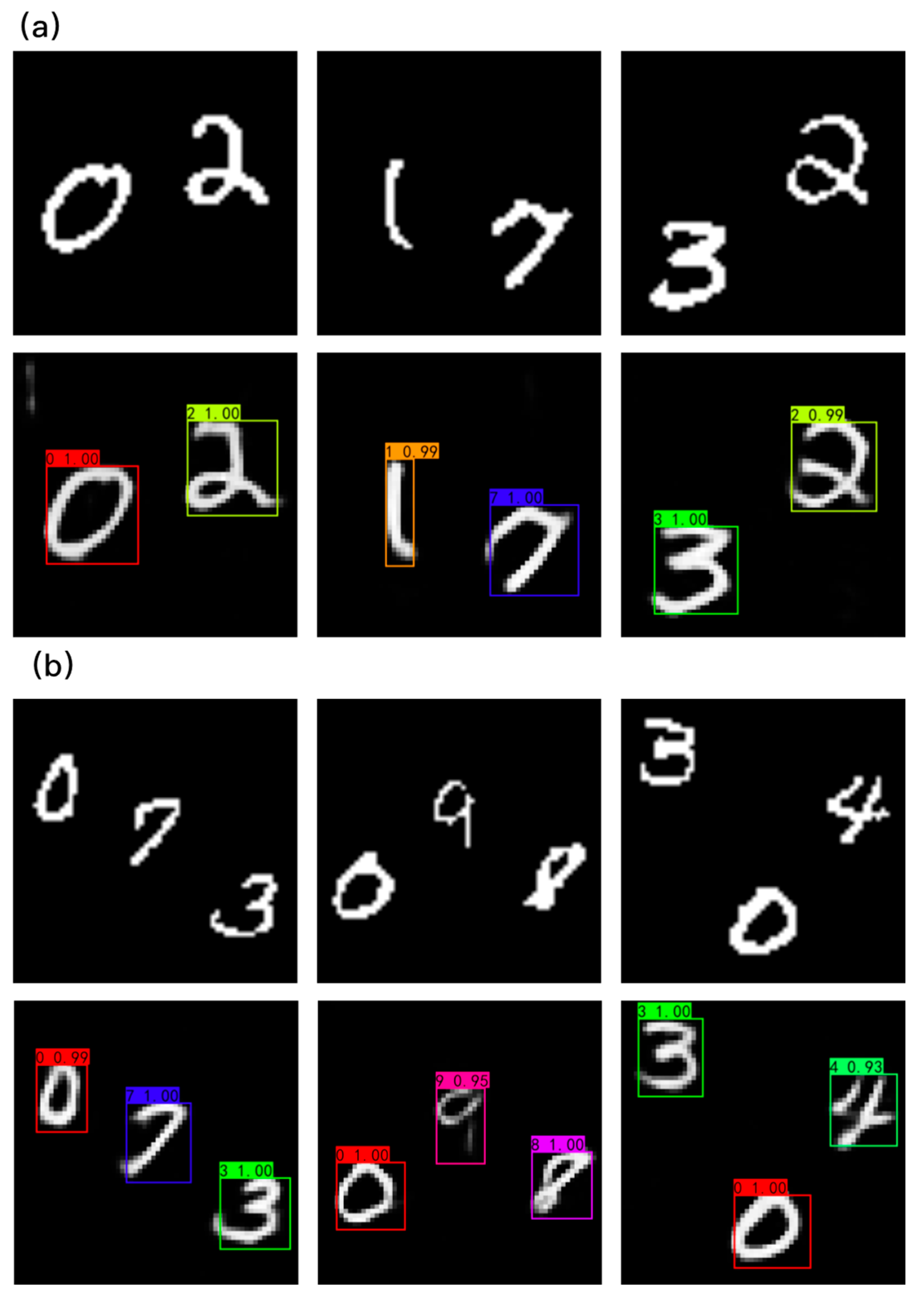
3.1. Concurrent Imaging, Location, and Classification

The left column of Figure 3 shows the original handwritten objects, which are the four single digit numbers 9, 7, 3, and 0. The right column of Figure 3 shows the results given by SP-ILC from the input S-vector (M = 333). It can be seen that for single objects with different sizes and locations, SP-ILC concurrently detects the image and its location and classifies it. SP-ILC performs single-pixel imaging, marks the position of the object with a rectangular frame, and appends the classification and classifying confidence to the image.
The left column of Figure 4 shows objects that are various handwritten numbers of different sizes. The right column of Figure 4 shows the results obtained by SP-ILC from the input S-vector (M = 333). It can be seen that for multiple objects of different sizes and positions, SP-ILC concurrently performs high-definition imaging, high precision object location and highly accurate classification. SP-ILC performs well on imaging, object location, and classification for overlapping objects [4 and 2 in Figure 4d, 2 and 5 in Figure 4h].
In order to quantify the performance of SP-ILC, we conducted a quantitative study on the test set, as shown in Table 1. The test set (we named it Testset-80 in the following) included 40 single object samples and 40 multiple object samples. Table 1 shows that the performances of SP-ILC on single objects samples are better than that on the multiple object samples since the single object task is easier to process.
The peak signal-to-noise ratio (PSNR) and the structural similarity function (SSIM) are widely used to measure image quality [51,52]. The PSNR is defined by:
P S N R = 20 log 10 M A X G R M S E ,
where the RMSE is defined in Equation (2) and M A X G , which is the maximum value of the image, is 255 in this paper. The SSIM is defined by:
S S I M ( G , G ^ ) = ( 2 u G u G ^ + α 1 ) ( 2 σ G G ^ + α 2 ) ( u G 2 + u G ^ 2 + α 1 ) ( σ G 2 + σ G ^ 2 + α 2 ) ,
where u and σ are the mean values and variances of images respectively, σ G G ^ is the cross-correlation coefficient between the original images (ground truth/labels) of objects and the image retrieved by the SP-ILC, and α 1 and α 2 are two positive constants to avoid a null denominator.
We use Precision and Recall to quantify the accuracy of location and classification respectively. Precision is the percentage of correct predictions in all predictions, and recall is the percentage of correct predictions in all labels [53,54].
The calculation of both precision and recall is based on IOU, the ratio of the intersection to the union of the labeled position (the original bounding Box A) and the predicted position (the predicted bounding Box B):
I O U = A r e a ( A B ) A r e a ( A B ) .
We classified only frames with IOU > 0.5; that is, only in cases when IOU > 0.5 and the predicted classification was correct were considered to be correct in both classification and location.
The confidence level is 0.6, which means only predicted bounding boxes with confidence larger than 0.6 are reserved.

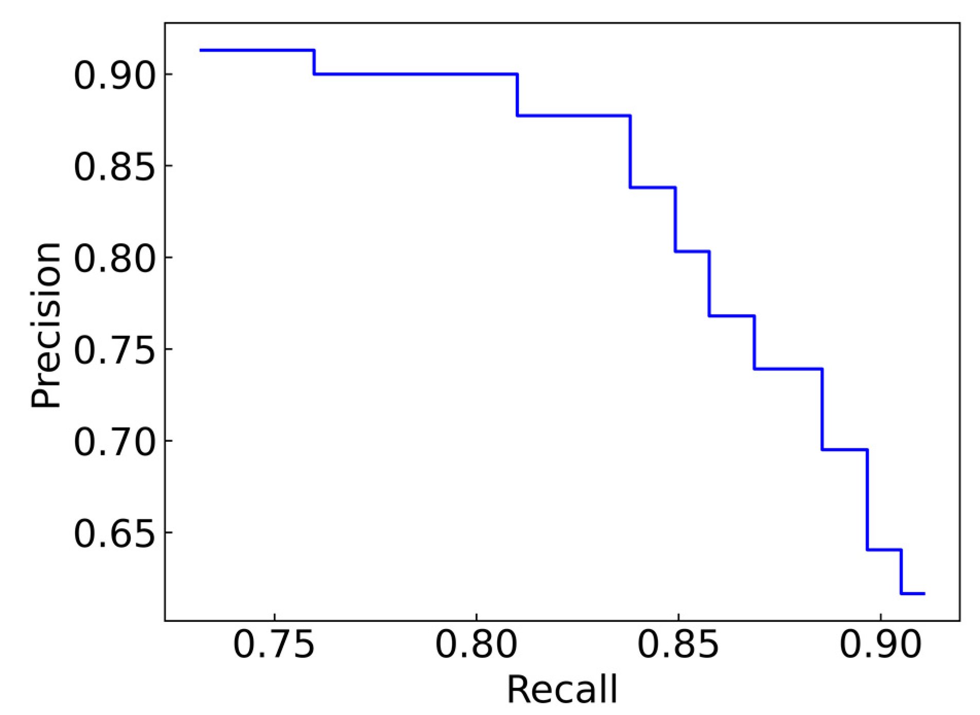
3.2. Precision–Recall Curve

We examined the precision–recall curves in terms of accuracy of object location and accuracy of classification. The PR curve in Figure 5 shows changes in precision and recall for the object location and classification tasks in response to changes in the confidence level during testing; it is a good measure of network performance.
In general, when the confidence level is increased, precision will also increase and recall will decrease. If the confidence level is decreased, precision will also decrease but recall will increase. The confidence level can be varied independently for the different tasks in order to reach the best operational system state. For example, for disease detection, recall is more important than precision; thus, recall needs to be very high, and there is some tolerance for low precision. We can decrease the confidence level to achieve the optimal solution for this type of task. The confidence level can be similarly adjusted for other tasks to achieve a balance between precision and recall.

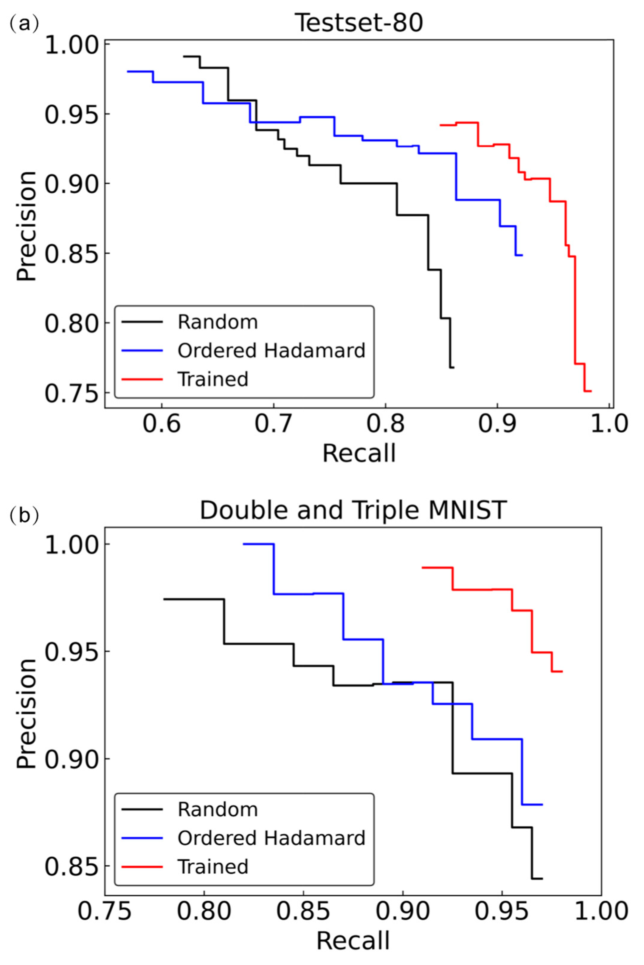
3.3. Generalizaiton Ability

To proof the generalization ability of SP-ILC, we use the trained SP-ILC to test the double MNIST and triple MNIST datasets. A total of 20 examples of double MNIST and 20 examples of triple MNIST are randomly chosen. As shown in Figure 6 and Table 2, SP-ILC works well in the double MNIST and triple MNIST datasets, although all the trained datasets of these two datasets are not used in the training of SP-ILC. Compared Table 1 to Table 2, the difficulties of multiple objects of Testset-80 are larger than that of the double and triple MNIST. Because the size of double and triple MNIST is similar and there is no overlap between different objects.
The Testset-80, double MNIST, and triple MNIST datasets contained only images of digits because the purpose of this paper is to demonstrate the feasibility of concurrent single-pixel imaging, object location, and object classification using deep learning.

3.4. Optimal Patterns
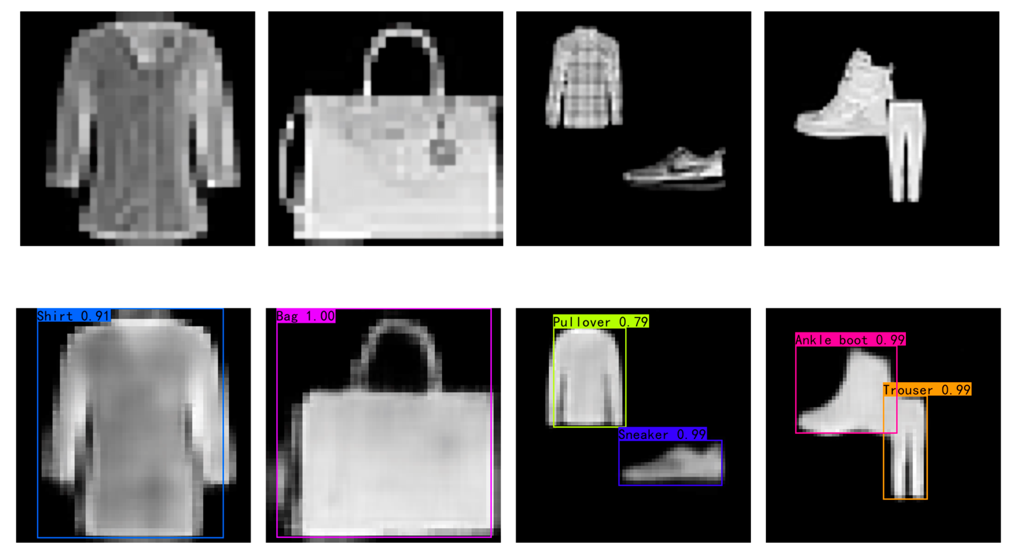
The results of Section 3.1, Section 3.2 and Section 3.3 are obtained by using the random pattern. In this section, we numerically study the improvement of the performance of SP-ILC using optimal patterns.
As shown in Figure 7 and Table 3, the performances of both the ordered Hadamard patterns and the trained patterns are generally better than that of the random patterns in different datasets. The Hadamard patterns are ordered by the number of connected regions [55]. These improvements are consistent with previous studies [35,37]. This simulation study shows that the optimal patterns, especially trained or ’learned’ patterns, can be used to further improve the performance of SP-ILC.

3.5. Fashion MNIST

Although the above studies focus on MNIST which consists only of images of digits, the proposed method may also work well in parsing scenes that contain images of real-world objects as long as a training dataset containing images of the actual objects is provided. To demonstrate this, we numerically studied the performance of SP-ILC on the dataset of the Fashion MNIST. The Fashion MNIST is a dataset that contains 70 K grayscale images (the pixel-value is an integer between 0 and 255), associated with labels from 10 classes [56].
Using the method described in Section 2.3, we prepared a dataset with 40 K samples to train the SP-ILC. The hyper-parameters and parameters are the same as that set on MNIST experiments. Particularly, the pattern number is also M = 333. A total of 100 test samples with a single object and 100 test samples with multiple objects are used to test the performance of SP-ILC. The test results are shown in Figure 8 and Table 4. The precision and recall are calculated in the confidence level of 0.6.
It can be seen that the SP-ILC works in the dataset based on the Fashion MNIST, which are grayscale images and closer to real-world images compared to the MNIST.

4. Discussions and Conclusions

4.1. Analysis of Imaging Ability

I. Hoshi et al. provided a detail study of the performance of the convolutional neural network (CNN)-based method and the recurrent neural network (RNN)-based method on MNIST and Fashion MNIST datasets using numerical experiments [57]. The number of patterns is also 333 and the size of the object is 64 × 64 in their experiments. In Section 3.5 of this paper, the random pattern is set to 0 and 1, and the optimal pattern is set to 1 and −1. This setting is the same as [57]. We compared both the CNN-based method [35] and RNN-based [57] method with SP-ILC in original Fashion MNIST.
The quantitative evaluation of the CNN-based and RNN-based methods are calculated according to Table 2 of [57]. The quantitative performance of the SP-ILC is calculated by testing 100 randomly chosen samples from the standard Fashion MNIST test set. The only operation for these 100 samples is resizing them from 28 × 28 to 64 × 64 for a fair comparison.
Table 5 shows the performance of SP-ILC exceeds both the CNN-based method and RNN-based method.

4.2. Analysis of Classification Ability

SP-ILC is the first work that can locate and classify multiple objects and objects of different sizes and overlap using a single-pixel detector, although there are previous studies that achieved the single-pixel classification for the scene with a single object and even the object is high-speed moving [34,37]. The metric for these works for single object classification is accuracy. However, for object location or object identification, it is hard to calculate the accuracy [58], since the calculation of accuracy relies on the true negative (TN) and for any given image, the number of TN is infinite because there is infinite number of bounding boxes that should not be detected [59].
Therefore, we designed the test set with 40 differently-sized MNIST test samples that contained only a single object to provide some degree of comparison (four examples are shown in Figure 2). When using a single-object test set, at a sampling rate of 8.1% (sampling rate is calculated by M/N = 333/4096), for 40 single target pictures, SP-ILC predicted 43 bounding boxes, of which 40 were correct. The precision of this performance was 0.930 (40/43). A total of 43 bounding boxes mean that SP-ILC may give more than one prediction for one object, for example, in Figure 4h, the number ‘4’ has been given two predictions, which will decrease the precision of the system. The recall was 1.000 (40/40). This classification performance matches that of current state-of-the-art classification tasks [34,37]. We note that in previous studies of the single-pixel classification there is prior knowledge that a scene contains only one object. SP-ILC does not have such prior knowledge, so even for a single object scene, our task is more difficult than current classification algorithms. Moreover, other studies have used similar-sized objects, whereas the object size in our test set varies.

4.3. The Test Time for One Image

The measurement number is M = 333 (displayed by 666 DMD patterns); the speed of the pattern change of the DMD is 20 kHz; the test time of SP-ILC for one frame of image costs about 28 ms (using one single GeForce RTX 2060 GPU). Therefore, the SP-ILC has the potential to achieve real-time concurrent imaging, object location, and classification.

4.4. The End-to-End Multitask Learning System

SP-ILC is an end-to-end multitask learning system. In comparison with sequential pipelines (do SPI first and then send the image to an object identification system), SP-ILC offers many benefits: (1) the multitask learning deep neural network is structurally more compact than sequential pipelines and dispenses with the training of multiple models; (2) the multitask learning technique can share shadow layers of the deep neural network between different tasks, which promotes efficient learning; and (3) multitask learning increases generalizability, which is very important for deep learning models because different tasks have components unrelated to other tasks that can be ignored as noise by the other tasks, thus making the model more robust [60,61].
In summary, this paper proposes SP-ILC to perform concurrent imaging, object location, and classification using deep learning. Through feature sharing, multitask loss function design, and the use of a custom purpose-built large-scale dataset, SP-ILC successfully performed high quality imaging, high precision object location, and accurate classification of objects of different sizes and numbers and even with overlap. SP-ILC has potential applications in practical fields such as security, medicine, and autonomous vehicles. We have made the dataset and all SP-ILC coding available as open source to help other researchers in their work.

Author Contributions

Z.Y. and Y.-M.B. contributed equally to this paper. Conceptualization, Z.Y. and J.-L.L.; methodology and investigation, Z.Y., Y.-M.B., L.-D.S., K.-X.H. and J.L.; visualization, Z.Y., Y.-M.B. and L.-D.S.; formal analysis, Z.Y., Y.-M.B. and L.-D.S.; data curation, Y.-M.B.; writing—original draft preparation, Z.Y., Y.-M.B. and L.-D.S.; writing—review and editing, Z.Y., Y.-M.B., D.R. and J.-L.L.; supervision, D.R. and J.-L.L.; funding acquisition, Z.Y., D.R. and J.-L.L. All authors have read and agreed to the published version of the manuscript.

Funding

This work was supported by the National Natural Science Foundation of China with grant number 51727805. Z.Y. acknowledges the support from the National Natural Science Foundation of China with grant number 12104251. D.R. acknowledges the support from the National Natural Science Foundation of China with grant number 62131002.

Data Availability Statement

Data available upon request.

Acknowledgments

We thank Kai-Li Jiang for his comments and support in this work.

Conflicts of Interest

The authors declare no conflict of interest.

References

  1. Sun, M.J.; Zhang, J.M. Single-Pixel Imaging and Its Application in Three-Dimensional Reconstruction: A Brief Review. Sensors 2019, 19, 732. [Google Scholar] [CrossRef] [Green Version]
  2. Gibson, G.M.; Johnson, S.D.; Padgett, M. Single-pixel imaging 12 years on: A review. Opt. Express 2020, 28, 28190–28208. [Google Scholar] [CrossRef] [PubMed]
  3. Zhao, J.; Yiwen, E.; Williams, K.; Zhang, X.C.; Boyd, R. Spatial sampling of terahertz fields with sub-wavelength accuracy via probe beam encoding. Light Sci. Appl. 2019, 8, 55. [Google Scholar] [CrossRef] [Green Version]
  4. Radwell, N.; Mitchell, K.J.; Gibson, G.M.; Edgar, M.P.; Bowman, R.; Padgett, M.J. Single-pixel infrared and visible microscope. Optica 2014, 1, 285–289. [Google Scholar] [CrossRef]
  5. Zhang, A.X.; He, Y.H.; Wu, L.A.; Chen, L.M.; Wang, B.B. Tabletop X-ray ghost imaging with ultra-low radiation. Optica 2018, 5, 374–377. [Google Scholar] [CrossRef] [Green Version]
  6. Pittman, T.B.; Shih, Y.H.; Strekalov, D.V.; Sergienko, A.V. Optical imaging by means of two-photon quantum entanglement. Phys. Rev. A 1995, 52, R3429–R3432. [Google Scholar] [CrossRef] [PubMed]
  7. Shapiro, J.H. Computational ghost imaging. Phys. Rev. A 2008, 78, 061802. [Google Scholar] [CrossRef]
  8. Katz, O.; Yaron, B.; Silberberg, Y. Compressive ghost imaging. Appl. Phys. Lett. 2009, 95, 131110. [Google Scholar] [CrossRef] [Green Version]
  9. Chen, Q.; Mathai, A.; Xu, X.; Wang, X. A Study into the Effects of Factors Influencing an Underwater, Single-Pixel Imaging System’s Performance. Photonics 2019, 6, 123. [Google Scholar] [CrossRef] [Green Version]
  10. Yan, S.M.; Sun, M.J.; Chen, W.; Li, L.J. Illumination Calibration for Computational Ghost Imaging. Photonics 2021, 8, 59. [Google Scholar] [CrossRef]
  11. Yang, Z.; Zhang, W.X.; Liu, Y.P.; Ruan, D.; Li, J.L. Instant ghost imaging: Algorithm and on-chip Implementation. Opt. Express 2020, 28, 3607–3618. [Google Scholar] [CrossRef] [Green Version]
  12. Yang, Z.; Liu, J.; Zhang, W.X.; Ruan, D.; Li, J.L. Instant single-pixel imaging: On-chip real-time implementation based on the instant ghost imaging algorithm. OSA Contin. 2020, 3, 629–636. [Google Scholar] [CrossRef]
  13. Shang, R.; Hoffer-Hawlik, K.; Wang, F.; Situ, G.; Luke, G. Two-step training deep learning framework for computational imaging without physics priors. Opt. Express 2021, 29, 15239–15254. [Google Scholar] [CrossRef] [PubMed]
  14. Sun, M.J.; Edgar, M.P.; Gibson, G.M.; Sun, B.; Radwell, N.; Lamb, R.; Padgett, M.J. Single-pixel three-dimensional imaging with time-based depth resolution. Nat. Commun. 2016, 7, 12010. [Google Scholar] [CrossRef] [PubMed]
  15. Wang, H.; Bian, L.; Zhang, J. Depth acquisition in single-pixel imaging with multiplexed illumination. Opt. Express 2021, 29, 4866–4874. [Google Scholar] [CrossRef] [PubMed]
  16. Gong, W.; Zhao, C.; Yu, H.; Chen, M.; Xu, W.; Han, S. Three-dimensional ghost imaging lidar via sparsity constraint. Sci. Rep. 2016, 6, 26133. [Google Scholar] [CrossRef] [PubMed] [Green Version]
  17. Wang, Y.; Chen, H.; Jiang, W.; Li, X.; Chen, X.; Meng, X.; Tian, P.; Sun, B. Optical encryption for visible light communication based on temporal ghost imaging with a micro-LED. Opt. Lasers Eng. 2020, 134, 106290. [Google Scholar] [CrossRef]
  18. LeCun, Y.; Bengio, Y.; Hinton, G. Deep learning. Nature 2015, 521, 436–444. [Google Scholar] [CrossRef]
  19. Shrestha, A.; Mahmood, A. Review of Deep Learning Algorithms and Architectures. IEEE Access 2019, 7, 53040–53065. [Google Scholar] [CrossRef]
  20. Zoran, D.; Chrzanowski, M.; Huang, P.S.; Gowal, S.; Kohli, P. Towards Robust Image Classification Using Sequential Attention Models. In Proceedings of the IEEE Conference on Computer Vision and Pattern Recognition, Seattle, WA, USA, 13–19 June 2020; pp. 9483–9492. [Google Scholar]
  21. Xiao, Y.; Tian, Z.; Yu, J.; Zhang, Y.; Liu, S.; Du, S.; Lan, X. A review of object detection based on deep learning. Multimed. Tools Appl. 2020, 79, 23729–23791. [Google Scholar] [CrossRef]
  22. Long, J.; Shelhamer, E.; Darrell, T. Fully convolutional networks for semantic segmentation. In Proceedings of the IEEE Conference on Computer Vision and Pattern Recognition, Boston, MA, USA, 7–12 June 2015; pp. 3431–3440. [Google Scholar]
  23. Li, X.S.; Yue, T.Z.; Huang, X.P.; Yang, Z.; Xu, G. BAGS: An automatic homework grading system using the pictures taken by smart phones. arXiv 2019, arXiv:1906.03767. [Google Scholar]
  24. Xu, G.; Song, Z.G.; Sun, Z.; Ku, C.; Yang, Z.; Liu, C.C.; Wang, S.H.; Ma, J.P.; Xu, W. Camel: A weakly supervised learning framework for histopathology image segmentation. In Proceedings of the IEEE/CVF International Conference on Computer Vision, Seoul, Korea, 27 October–3 November 2019; pp. 10682–10691. [Google Scholar]
  25. Goda, K.; Jalali, B.; Lei, C.; Situ, G.; Westbrook, P. AI boosts photonics and vice versa. APL Photonics 2020, 5, 070401. [Google Scholar] [CrossRef]
  26. Bian, T.; Yi, Y.; Hu, J.; Zhang, Y.; Gao, L. A residual-based deep learning approach for ghost imaging. Sci. Rep. 2020, 10, 12149. [Google Scholar] [CrossRef] [PubMed]
  27. Wu, H.; Wang, R.; Zhao, G.; Xiao, H.; Zhang, X. Sub-nyquist computational ghost imaging with deep learning. Opt. Express 2020, 28, 3846–3853. [Google Scholar] [CrossRef]
  28. Wu, H.; Zhao, G.; Chen, M.; Cheng, L.; Xiao, H.; Xu, L.; Wang, D.; Liang, J.; Xu, Y. Hybrid neural network-based adaptive computational ghost imaging. Opt. Lasers Eng. 2021, 140, 106529. [Google Scholar] [CrossRef]
  29. Wu, H.; Wang, R.; Zhao, G.; Xiao, H.; Liang, J.; Wang, D.; Tian, X.; Cheng, L.; Zhang, X. Deep-learning denoising computational ghost imaging. Opt. Lasers Eng. 2020, 134, 106183. [Google Scholar] [CrossRef]
  30. Latorre-Carmona, P.; Traver, V.J.; Sánchez, J.S.; Tajahuerce, E. Online reconstruction-free single-pixel image classification. Image Vis. Comput. 2019, 86, 28–37. [Google Scholar] [CrossRef]
  31. Ducros, N.; Mur, A.L.; Peyrin, F. A completion network for reconstruction from compressed acquisition. In Proceedings of the 2020 IEEE 17th International Symposium on Biomedical Imaging (ISBI), Iowa City, IA, USA, 3–7 April 2020; pp. 619–623. [Google Scholar]
  32. Mur, A.; Leclerc, P.; Peyrin, F.; Ducros, N. Single-pixel image reconstruction from experimental data using neural networks. Opt. Express 2021, 29, 17097–17110. [Google Scholar] [CrossRef] [PubMed]
  33. Lyu, M.; Wang, W.; Wang, H.; Wang, H.; Li, G.; Chen, N.; Situ, G. Deep-learning-based ghost imaging. Sci. Rep. 2017, 7, 1–6. [Google Scholar] [CrossRef]
  34. Jiao, S. Fast object classification in single-pixel imaging. In Proceedings of the Sixth International Conference on Optical and Photonic Engineering (icOPEN), Shanghai, China, 8–11 May 2018; p. 108271O. [Google Scholar]
  35. Higham, C.F.; Murray-Smith, R.; Padgett, M.J.; Edgar, M.P. Deep learning for real-time single-pixel video. Sci. Rep. 2018, 8, 1–9. [Google Scholar] [CrossRef] [PubMed] [Green Version]
  36. Wang, F.; Wang, H.; Wang, H.; Li, G.; Situ, G. Learning from simulation: An end-to-end deep-learning approach for computational ghost imaging. Opt. Express 2019, 27, 25560–25572. [Google Scholar] [CrossRef] [PubMed]
  37. Zhang, Z.; Li, X.; Zheng, S.; Yao, M.; Zheng, G.; Zhong, J. Image-free classification of fast-moving objects using “learned” structured illumination and single-pixel detection. Opt. Express 2020, 28, 13269–13278. [Google Scholar] [CrossRef] [PubMed]
  38. Shimobaba, T.; Endo, Y.; Nishitsuji, T.; Takahashi, T.; Nagahama, Y.; Hasegawa, S.; Sano, M.; Hirayama, R.; Kakue, T.; Shiraki, A.; et al. Computational ghost imaging using deep learning. Opt. Commun. 2018, 413, 147–151. [Google Scholar] [CrossRef] [Green Version]
  39. He, Y.; Wang, G.; Dong, G.; Zhu, S.; Chen, H.; Zhang, A.; Xu, Z. Ghost imaging based on deep learning. Sci. Rep. 2018, 8, 6469. [Google Scholar] [CrossRef] [PubMed] [Green Version]
  40. Radwell, N.; Johnson, S.D.; Edgar, M.P.; Higham, C.F.; Murray-Smith, R.; Padgett, M.J. Deep learning optimized single-pixel lidar. Appl. Phys. Lett. 2019, 115, 231101. [Google Scholar] [CrossRef] [Green Version]
  41. He, K.; Zhang, X.; Ren, S.; Sun, J. Deep Residual Learning for Image Recognition. In Proceedings of IEEE Conference on Computer Vision and Pattern Recognition, Las Vegas, USA, 27–30 June 2016; pp. 770–778. [Google Scholar]
  42. Ren, S.; He, K.; Girshick, R.; Sun, J. Faster r-cnn: Towards real-time object detection with region proposal networks. IEEE Trans. Pattern Anal. Mach. Intell. 2017, 39, 1137–1149. [Google Scholar] [CrossRef] [PubMed] [Green Version]
  43. Redmon, J.; Divvala, S.; Girshick, R.; Farhadi, A. You Only Look Once: Unified, Real-Time Object Detection. In Proceedings of the IEEE Conference on Computer Vision and Pattern Recognition, Las Vegas, USA, 27–30 June 2016; pp. 779–788. [Google Scholar]
  44. Redmon, J.; Farhadi, A. Yolov3: An incremental improvement. arXiv 2018, arXiv:1804.02767. [Google Scholar]
  45. SP-ILC: Concurrent Single-Pixel Imaging, Object Location, and Classification by Deep Learning. Available online: https://github.com/Polarbeartnt/SP-ILC (accessed on 14 September 2021).
  46. Wang, L.; Zhao, S. Fast reconstructed and high-quality ghost imaging with fast Walsh–Hadamard transform. Photon. Res. 2016, 4, 240–244. [Google Scholar] [CrossRef]
  47. Iqbal, H. HarisIqbal88/PlotNeuralNet v1.0.0 (Version v1.0.0). Zenodo, 2018. [Google Scholar] [CrossRef]
  48. Le Cun, Y.; Cortes, C.; Burges, C.J.C. The MNIST Database of Handwritten Digits. 1998. Available online: http://yann.lecun.com/exdb/mnist/ (accessed on 15 October 2020).
  49. Paszke, A.; Gross, S.; Chintala, S.; Chanan, G.; Yang, E.; DeVito, Z.; Lin, Z.; Desmaison, A.; Antiga, L.; Lerer, A. Automatic differentiation in pytorch. In Proceedings of the 31st Conference on Neural Information Processing Systems, Long Beach, CA, USA, 4–9 December 2017; pp. 1–4. [Google Scholar]
  50. Kingma, D.; Ba, J. Adam: A method for stochastic optimization. arXiv 2014, arXiv:1412.6980. [Google Scholar]
  51. Hore, A.; Ziou, D. Image quality metrics: PSNR vs. SSIM. In Proceedings of the 20th International Conference on Pattern Recognition, Istanbul, Turkey, 23–26 August 2010; pp. 2366–2369. [Google Scholar]
  52. Zhu, R.; Yu, H.; Tan, Z.; Lu, R.; Han, S.; Huang, Z.; Wang, J. Ghost imaging based on Y-net: A dynamic coding and decoding approach. Opt. Express 2020, 28, 17556–17569. [Google Scholar] [CrossRef]
  53. Buckland, M.; Gey, F. The relationship between recall and precision. J. Am. Soc. Inf. Sci. 1994, 45, 12–19. [Google Scholar] [CrossRef]
  54. Torgo, L.; Ribeiro, R. Precision and recall for regression. In Proceedings of the International Conference on Discovery Science, Porto, Portugal, 3–5 October 2009; pp. 332–346. [Google Scholar]
  55. Yu, W.K. Super sub-nyquist single-pixel imaging by means of cake-cutting hadamard basis sort. Sensors 2019, 19, 4122. [Google Scholar] [CrossRef] [PubMed] [Green Version]
  56. Xiao, H.; Rasul, K.; Vollgraf, R. Fashion-mnist: A novel image dataset for benchmarking machine learning algorithms. arXiv 2017, arXiv:1708.07747. [Google Scholar]
  57. Hoshi, I.; Shimobaba, T.; Kakue, T.; Ito, T. Single-pixel imaging using a recurrent neural network combined with convolutional layers. Opt. Express 2020, 28, 34069–34078. [Google Scholar] [CrossRef] [PubMed]
  58. Metz, C.E. Basic principles of ROC analysis. Semin. Nucl. Med. 1978, 8, 283–298. [Google Scholar] [CrossRef]
  59. Padilla, R.; Netto, S.L.; da Silva, E.A.B. A Survey on Performance Metrics for Object-Detection Algorithms. In Proceedings of the 2020 International Conference on Systems, Signals and Image Processing, Niteroi, Brazil, 1–3 July 2020; pp. 237–242. [Google Scholar]
  60. Caruana, R. Multitask learning. Mach. Learn 1997, 28, 41–75. [Google Scholar] [CrossRef]
  61. Girshick, R. Fast r-cnn. In Proceedings of the IEEE International Conference on Computer Vision, Santiago, Chile, 13–16 December 2015; pp. 1440–1448. [Google Scholar]
Figure 1. SP-ILC schematic. (a) The 532 nm laser is modulated by patterns displayed by the digital micromirror device (DMD). The object is displayed on the spatial light modulator (SLM) and the reflected light is collected by the single-pixel detector (PD) to create the bucket signal S. P is a linear polarizer. PBS is a polarization beam splitter. A/DC is an analog-to-digital convertor. PC is a personal computer with a GeForce RTX 2060 graphics processing unit (GPU). (b) The deep neural network concurrently performs imaging, classification, and location tasks using the single S-vector. The visualization is drawn using PlotNeuralNet software [47]. The numbers with slope alignment are the sizes of the feature maps and the numbers with horizontal alignment are the channel numbers of the feature maps. (c) The input and output of the SP-ILC with the trained deep neural network.
Photonics 08 00400 g001
Figure 2. A typical training process with loss decrease.
Photonics 08 00400 g002
Figure 3. Examples of single-pixel imaging, object location, and classification for a single object with different sizes and positions. The left column shows original images of objects displayed on SLM; the right column shows the retrieved images by SP-ILC. Concurrently, the location and classification of objects are also output by SP-ILC. The locating result (predicted bounding box) of one object is marked by a rectangle; two numbers above each rectangle (bounding box) are the classifying result and the corresponding classifying confidence, respectively.
Photonics 08 00400 g003
Figure 4. The left column (a,c,e,g) show original images of objects displayed on the SLM; the right column (b,d,f,h) show results of single-pixel imaging, classification, and location for scenes containing multiple objects with different sizes and locations and overlap.
Photonics 08 00400 g004
Figure 5. Precision–recall curves of SP-ILC for Testset-80.
Photonics 08 00400 g005
Figure 6. The performance of SP-ILC for (a) double MNIST and (b) triple MNIST. The first and third rows show the original image of objects; the second and fourth rows show results of the concurrent imaging, object locating and object classifying.
Photonics 08 00400 g006
Figure 7. The precision–recall curves of SP-ILC tested on (a) Testset-80 and (b) double and triple MNIST dataset for different kinds of patterns.
Photonics 08 00400 g007
Figure 8. The performance of SP-ILC, which is based on trained patterns, for the Fashion MNIST. The first row shows the original image of objects; the second row shows results of the concurrent imaging, object locating and object classifying.
Photonics 08 00400 g008
Table 1. The quantitative performance of SP-ILC for Testset-80.
PSNR [dB]SSIMPrecisionRecall
Single object22.9100.9480.9301.000
Multiple objects16.4870.8200.8080.799
Table 2. The quantitative performance of SP-ILC for double MNIST and Triple MNIST.
PSNR [dB]SSIMPrecisionRecall
Double MNIST20.7980.9150.9250.950
Triple MNIST19.4430.8760.9430.867
Table 3. The quantitative performance of SP-ILC for different datasets using optimal patterns.
Pattern NameMetrics of Image QualitySingle ObjectMultiple ObjectsDouble MNISTTriple MNIST
RandomPSNR [dB]24.81517.32020.79819.443
SSIM0.9600.8430.9150.876
Ordered HadamardPSNR [dB]24.72518.60620.89919.936
SSIM0.9680.9010.9360.920
TrainedPSNR [dB]29.24722.14525.15822.908
SSIM0.9880.9590.9790.964
Table 4. The quantitative performance of SP-ILC for Fashion MNIST.
Pattern NameSingle or Multiple ObjectsPSNR [dB]SSIMPrecisionRecall
RandomSingle19.8410.7170.8100.930
Multiple19.9270.8050.7910.812
TrainedSingle20.7930.7550.8470.930
Multiple21.0520.8440.7390.905
Table 5. The quantitative performance comparison of SP-ILC to CNN and RNN based methods for Fashion MNIST.
Pattern NameMetricsCNN-BasedRNN-BasedSP-ILC
RandomPSNR [dB]9.28315.27419.841
SSIM0.0600.2820.717
TrainedPSNR [dB]19.68720.45420.793
SSIM0.4900.4980.755
Publisher’s Note: MDPI stays neutral with regard to jurisdictional claims in published maps and institutional affiliations.

