Going Deeper into OSNR Estimation with CNN


Abstract
:1. Introduction
- Transparency to symbol rate, modulation format and impairments;
- Joint estimation of multiple parameters;
- Independence of signal receiving;
- Robust performance along with low complexity;
- End-to-end learning.
2. Principle of Proposed Scheme
2.1. OSNR Measurement
2.2. Design Principles of Basic CNN
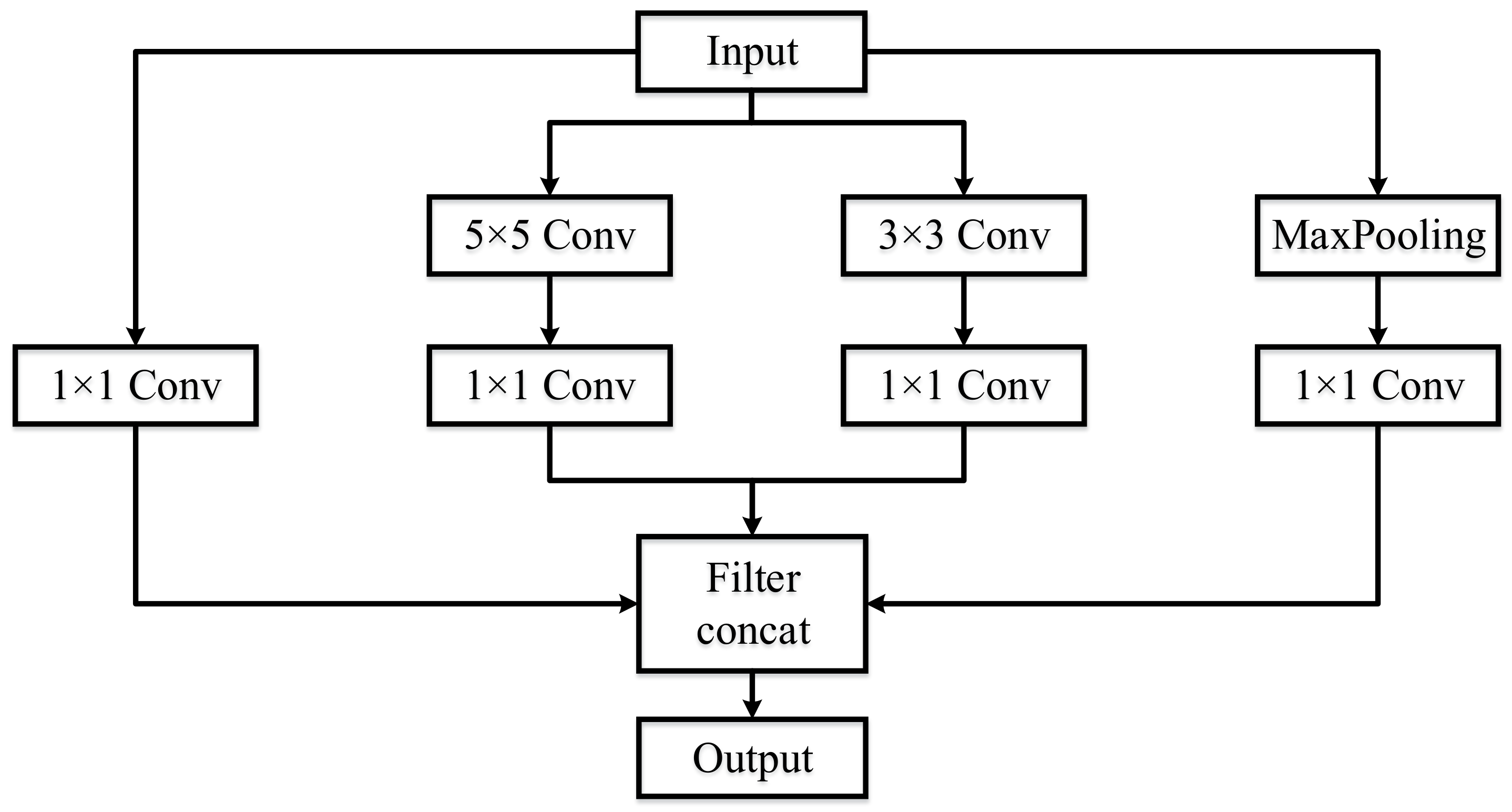
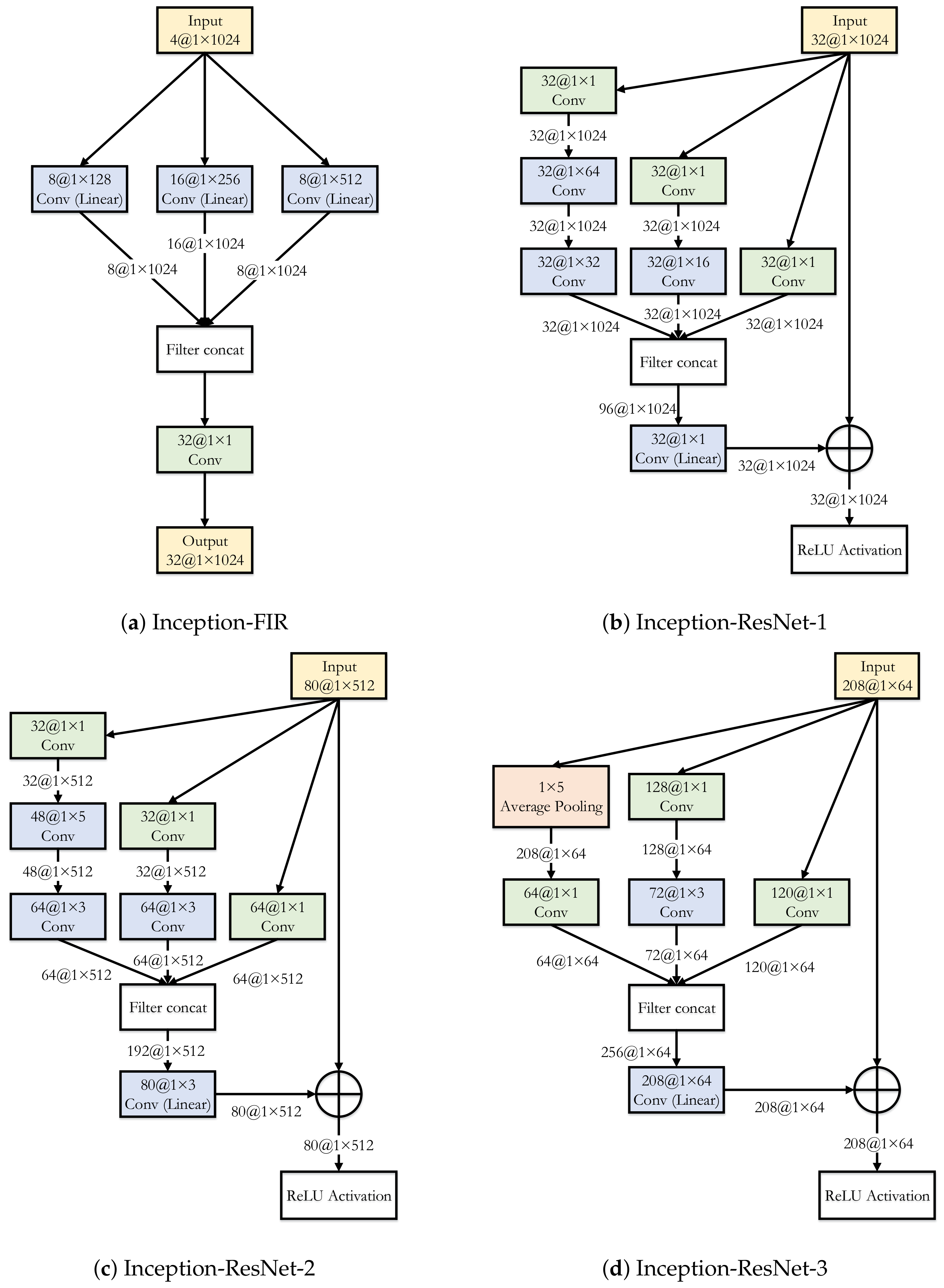
2.3. Inception Architecture
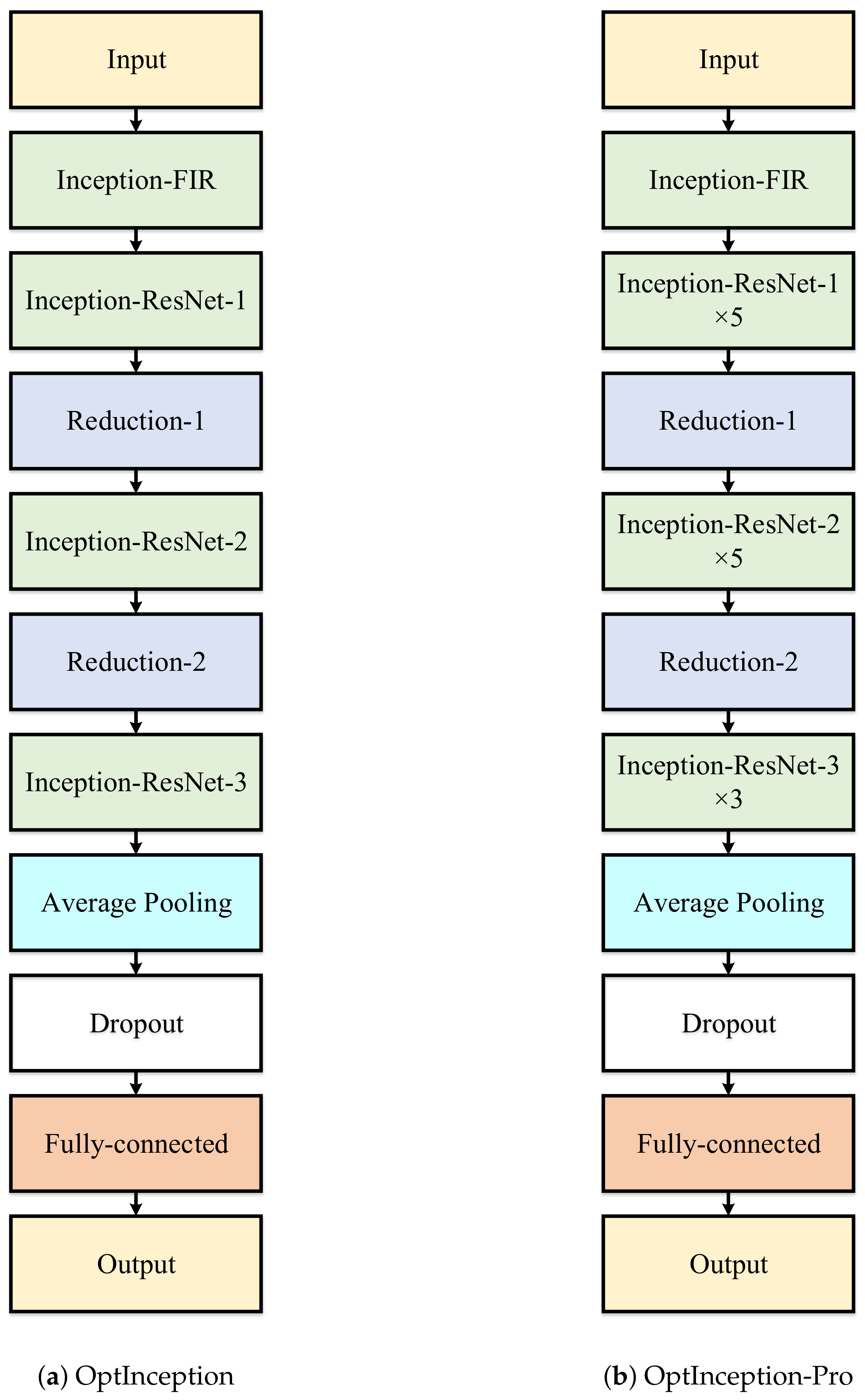
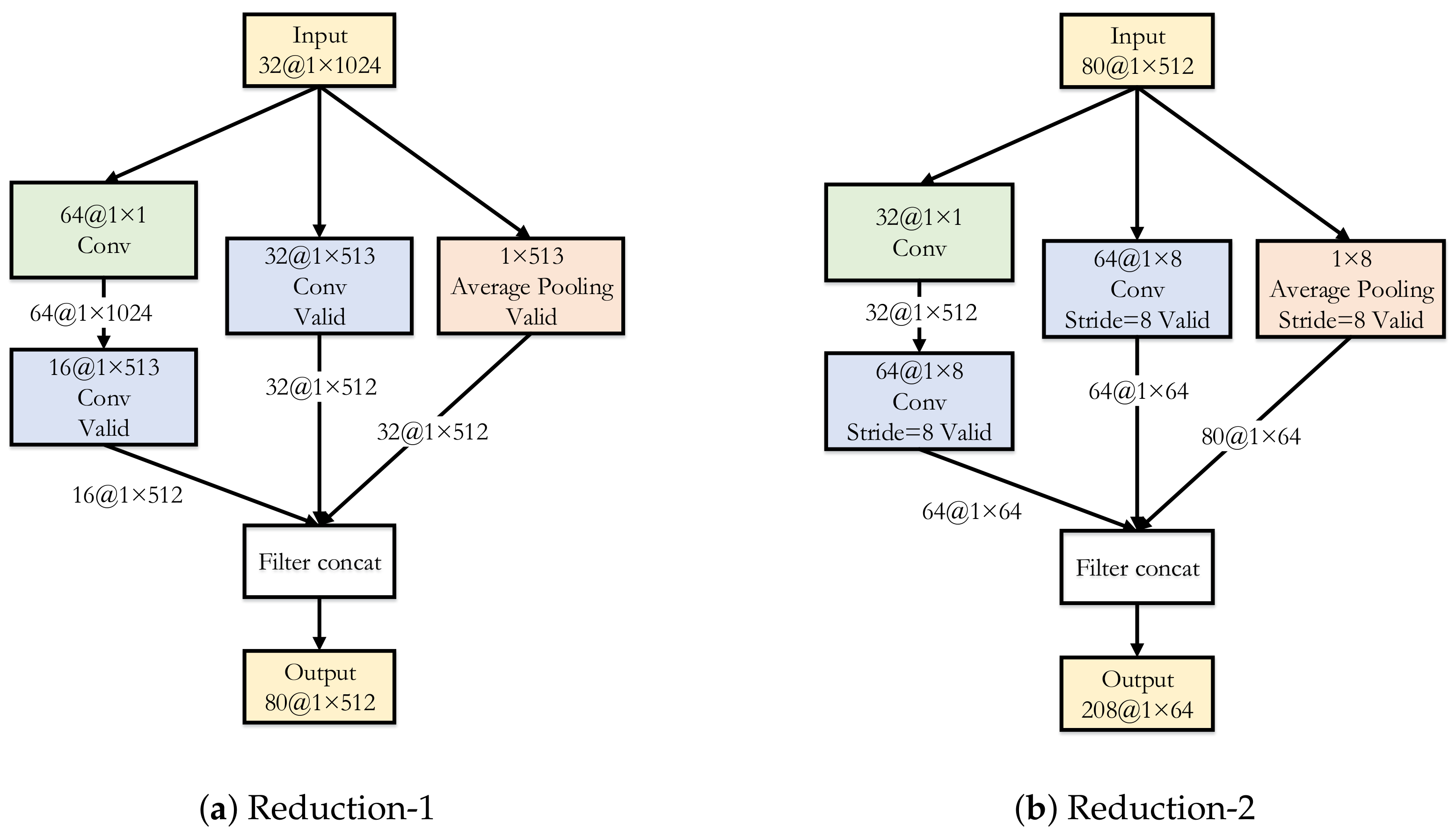
2.4. Proposed Scheme: OptInception
3. Experimental Result and Analysis
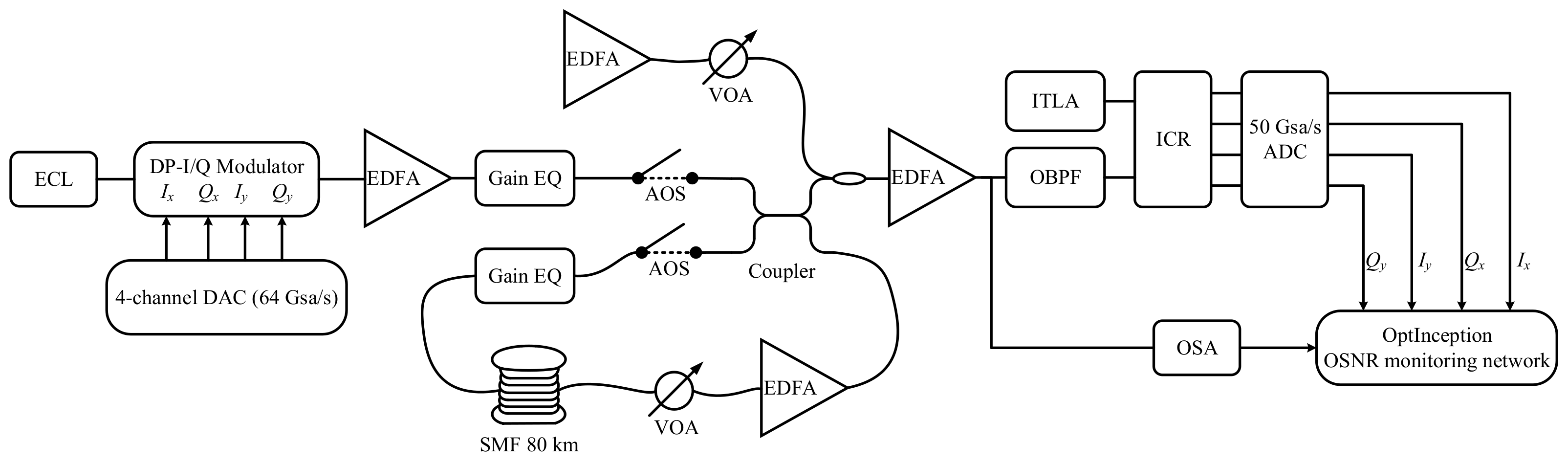
3.1. Experimental Setup
3.2. Training Methodology
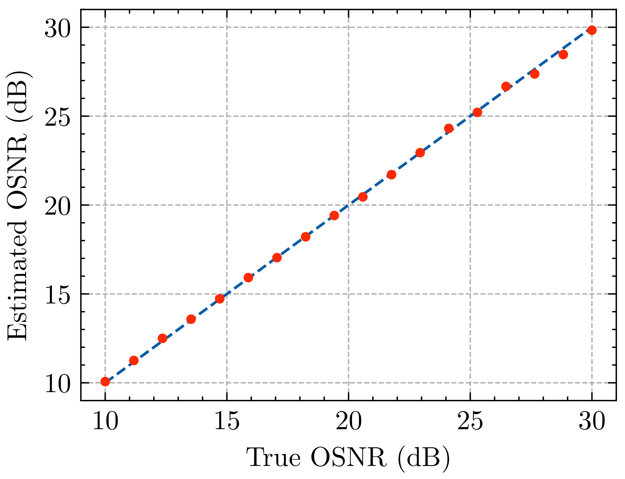
3.3. Results and Analysis
4. Discussion
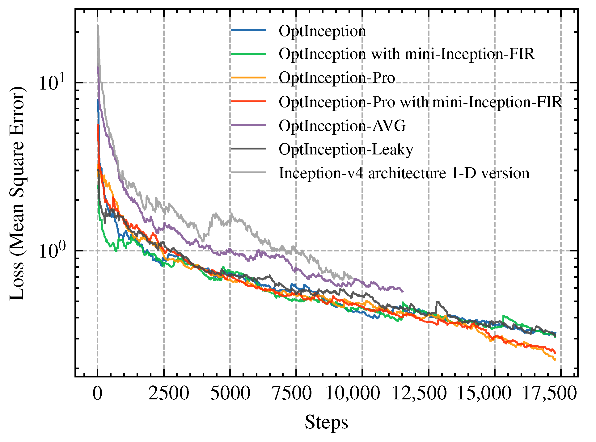
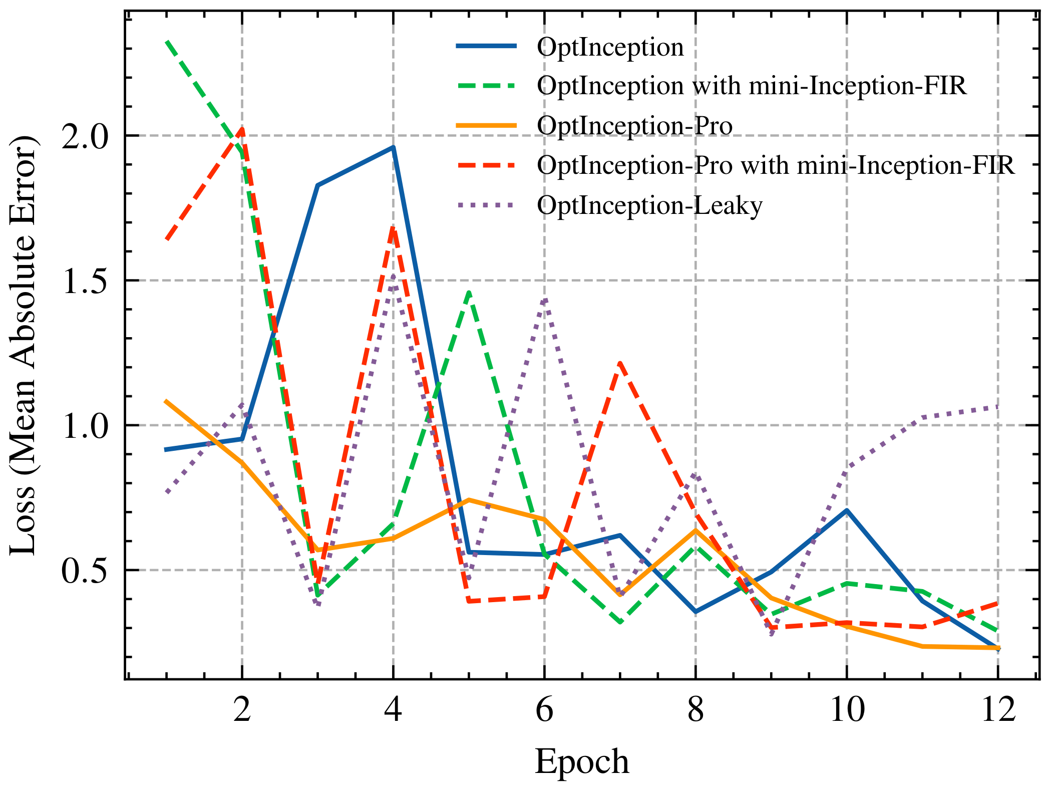
4.1. Learning Curve
4.2. Comparison
5. Conclusions
Author Contributions
Funding
Institutional Review Board Statement
Informed Consent Statement
Data Availability Statement
Conflicts of Interest
References
- Ramaswami, R.; Sivarajan, K.; Sasaki, G. Optical Networks: A Practical Perspective; Morgan Kaufmann: Burlington, MA, USA, 2009. [Google Scholar]
- Saif, W.S.; Esmail, M.A.; Ragheb, A.M.; Alshawi, T.A.; Alshebeili, S.A. Machine learning techniques for optical performance monitoring and modulation format identification: A survey. IEEE Commun. Surv. Tutor. 2020, 22, 2839–2882. [Google Scholar] [CrossRef]
- Dong, Z.; Khan, F.N.; Sui, Q.; Zhong, K.; Lu, C.; Lau, A.P.T. Optical Performance Monitoring: A Review of Current and Future Technologies. J. Light. Technol. 2016, 34, 525–543. [Google Scholar] [CrossRef]
- Khan, F.N.; Lu, C.; Lau, A.P.T. Optical Performance Monitoring in Fiber-Optic Networks Enabled by Machine Learning Techniques. In Proceedings of the 2018 Optical Fiber Communications Conference and Exposition (OFC), San Diego, CA, USA, 11–15 March 2018. [Google Scholar]
- Chomycz, B. Planning Fiber Optics Networks; McGraw-Hill Education: New York, NY, USA, 2009. [Google Scholar]
- Suzuki, H.; Takachio, N. Optical signal quality monitor built into WDM linear repeaters using semiconductor arrayed waveguide grating filter monolithically integrated with eight photodiodes. Electron. Lett. 1999, 35, 836–837. [Google Scholar] [CrossRef]
- Baker-Meflah, L.; Savory, S.; Thomsen, B.; Mitchell, J.; Bayvel, P. In-band OSNR monitoring using spectral analysis after frequency down-conversion. IEEE Photonics Technol. Lett. 2007, 19, 115–117. [Google Scholar] [CrossRef] [Green Version]
- Rasztovits-Wiech, M.; Danner, M.; Leeb, W. Optical signal-to-noise ratio measurement in WDM networks using polarization extinction. In Proceedings of the 24th European Conference on Optical Communication, ECOC’98 (IEEE Cat. No. 98TH8398), Madrid, Spain, 20–24 September 1998; Volume 1, pp. 549–550. [Google Scholar]
- Tao, Z.; Chen, Z.; Fu, L.; Wu, D.; Xu, A. Monitoring of OSNR by using a Mach–Zehnder interferometer. Microw. Opt. Technol. Lett. 2001, 30, 63–65. [Google Scholar] [CrossRef]
- Qiu, J.; Huang, Z.; Yuan, B.; An, N.; Kong, D.; Wu, J. Multi-wavelength in-band OSNR monitor based on Lyot-Sagnac interferometer. Opt. Express 2015, 23, 20257–20266. [Google Scholar] [CrossRef]
- Faruk, M.S.; Mori, Y.; Kikuchi, K. Estimation of OSNR for Nyquist-WDM transmission systems using statistical moments of equalized signals in digital coherent receivers. In Proceedings of the Optical Fiber Communication Conference, San Francisco, CA, USA, 9–13 March 2014; p. Th2A.29. [Google Scholar]
- Faruk, M.S.; Mori, Y.; Kikuchi, K. In-band estimation of optical signal-to-noise ratio from equalized signals in digital coherent receivers. IEEE Photonics J. 2014, 6, 1–9. [Google Scholar] [CrossRef]
- Ives, D.J.; Thomsen, B.C.; Maher, R.; Savory, S.J. Estimating OSNR of equalised QPSK signals. Opt. Express 2011, 19, B661–B666. [Google Scholar] [CrossRef]
- Zhu, C.; Tran, A.V.; Chen, S.; Du, L.B.; Do, C.C.; Anderson, T.; Lowery, A.J.; Skafidas, E. Statistical moments-based OSNR monitoring for coherent optical systems. Opt. Express 2012, 20, 17711–17721. [Google Scholar] [CrossRef] [PubMed]
- Lin, X.; Dobre, O.A.; Ngatched, T.M.N.; Li, C. A Non-Data-Aided OSNR Estimation Algorithm for Coherent Optical Fiber Communication Systems Employing Multilevel Constellations. J. Light. Technol. 2019, 37, 3815–3825. [Google Scholar] [CrossRef]
- Gaiarin, S.; Da Ros, F.; Jones, R.T.; Zibar, D. End-to-End Optimization of Coherent Optical Communications Over the Split-Step Fourier Method Guided by the Nonlinear Fourier Transform Theory. J. Light. Technol. 2021, 39, 418–428. [Google Scholar] [CrossRef]
- Wang, D.; Zhang, M.; Li, Z.; Li, J.; Fu, M.; Cui, Y.; Chen, X. Modulation Format Recognition and OSNR Estimation Using CNN-Based Deep Learning. IEEE Photonics Technol. Lett. 2017, 29, 1667–1670. [Google Scholar] [CrossRef]
- Wu, X.; Jargon, J.A.; Paraschis, L.; Willner, A.E. ANN-based optical performance monitoring of QPSK signals using parameters derived from balanced-detected asynchronous diagrams. IEEE Photonics Technol. Lett. 2010, 23, 248–250. [Google Scholar] [CrossRef]
- Khan, F.N.; Zhong, K.; Zhou, X.; Al-Arashi, W.H.; Yu, C.; Lu, C.; Lau, A.P.T. Joint OSNR monitoring and modulation format identification in digital coherent receivers using deep neural networks. Opt. Express 2017, 25, 17767–17776. [Google Scholar] [CrossRef]
- Wan, Z.; Yu, Z.; Shu, L.; Zhao, Y.; Zhang, H.; Xu, K. Intelligent optical performance monitor using multi-task learning based artificial neural network. Opt. Express 2019, 27, 11281–11291. [Google Scholar] [CrossRef] [PubMed] [Green Version]
- Li, J.; Wang, D.; Zhang, M. Low-complexity adaptive chromatic dispersion estimation scheme using machine learning for coherent long-reach passive optical networks. IEEE Photonics J. 2019, 11, 1–11. [Google Scholar] [CrossRef]
- Hao, M.; Yan, L.; Yi, A.; Jiang, L.; Pan, Y.; Pan, W.; Luo, B. OSNR Monitoring Using Support Vector Ordinal Regression for Digital Coherent Receivers. IEEE Photonics J. 2019, 11, 1–11. [Google Scholar] [CrossRef]
- Tanimura, T.; Hoshida, T.; Kato, T.; Watanabe, S.; Morikawa, H. Data-analytics-based optical performance monitoring technique for optical transport networks. In Proceedings of the Optical Fiber Communication Conference, San Diego, CA, USA, 11–15 March 2018; p. Tu3E.3. [Google Scholar]
- Tanimura, T.; Kato, T.; Watanabe, S.; Hoshida, T. Deep neural network based optical monitor providing self-confidence as auxiliary output. In Proceedings of the 2018 European Conference on Optical Communication (ECOC), Rome, Italy, 23–27 September 2018; pp. 1–3. [Google Scholar] [CrossRef]
- Tanimura, T.; Hoshida, T.; Kato, T.; Watanabe, S.; Morikawa, H. Convolutional Neural Network-Based Optical Performance Monitoring for Optical Transport Networks. J. Opt. Commun. Netw. 2019, 11, A52–A59. [Google Scholar] [CrossRef]
- Lecun, Y.; Bottou, L.; Bengio, Y.; Haffner, P. Gradient-based learning applied to document recognition. Proc. IEEE 1998, 86, 2278–2324. [Google Scholar] [CrossRef] [Green Version]
- Krizhevsky, A.; Sutskever, I.; Hinton, G.E. Imagenet classification with deep convolutional neural networks. Adv. Neural Inf. Process. Syst. 2012, 25, 1097–1105. [Google Scholar] [CrossRef]
- Simonyan, K.; Zisserman, A. Very Deep Convolutional Networks for Large-Scale Image Recognition. In Proceedings of the International Conference on Learning Representations, San Diego, CA, USA, 7–9 May 2015. [Google Scholar]
- Lin, M.; Chen, Q.; Yan, S. Network in network. arXiv 2013, arXiv:1312.4400. [Google Scholar]
- Szegedy, C.; Liu, W.; Jia, Y.; Sermanet, P.; Reed, S.; Anguelov, D.; Erhan, D.; Vanhoucke, V.; Rabinovich, A. Going deeper with convolutions. In Proceedings of the 2015 IEEE Conference on Computer Vision and Pattern Recognition (CVPR), Boston, MA, USA, 7–12 June 2015; pp. 1–9. [Google Scholar] [CrossRef] [Green Version]
- Savory, S.J. Digital Coherent Optical Receivers: Algorithms and Subsystems. IEEE J. Sel. Top. Quantum Electron. 2010, 16, 1164–1179. [Google Scholar] [CrossRef]
- Chan, C.C. Optical Performance Monitoring: Advanced Techniques for Next-Generation Photonic Networks; Academic Press: Cambridge, MA, USA, 2010. [Google Scholar]
- Khan, F.N.; Fan, Q.; Lu, C.; Lau, A.P.T. An Optical Communication’s Perspective on Machine Learning and Its Applications. J. Light. Technol. 2019, 37, 493–516. [Google Scholar] [CrossRef]
- LeCun, Y.; Bengio, Y.; Hinton, G. Deep learning. Nature 2015, 521, 436–444. [Google Scholar] [CrossRef] [PubMed]
- Goodfellow, I.; Bengio, Y.; Courville, A. Deep Learning; MIT Press: Cambridge, MA, USA, 2016. [Google Scholar]
- Hornik, K.; Stinchcombe, M.; White, H. Multilayer feedforward networks are universal approximators. Neural Netw. 1989, 2, 359–366. [Google Scholar] [CrossRef]
- Szegedy, C.; Vanhoucke, V.; Ioffe, S.; Shlens, J.; Wojna, Z. Rethinking the Inception Architecture for Computer Vision. In Proceedings of the 2016 IEEE Conference on Computer Vision and Pattern Recognition (CVPR), Las Vegas, NV, USA, 27–30 June 2016; pp. 2818–2826. [Google Scholar] [CrossRef] [Green Version]
- Szegedy, C.; Ioffe, S.; Vanhoucke, V.; Alemi, A.A. Inception-v4, Inception-ResNet and the impact of residual connections on learning. In Proceedings of the Thirty-First AAAI Conference on Artificial Intelligence, San Francisco, CA, USA, 4–9 February 2017. [Google Scholar]
- He, K.; Zhang, X.; Ren, S.; Sun, J. Deep residual learning for image recognition. In Proceedings of the IEEE Conference on Computer Vision and Pattern Recognition, Las Vegas, NV, USA, 27–30 June 2016; pp. 770–778. [Google Scholar]
- He, K.; Zhang, X.; Ren, S.; Sun, J. Identity mappings in deep residual networks. In Proceedings of the European Conference on Computer Vision, Amsterdam, The Netherlands, 8–16 October 2016; pp. 630–645. [Google Scholar]
- Abadi, M.; Barham, P.; Chen, J.; Chen, Z.; Davis, A.; Dean, J.; Devin, M.; Ghemawat, S.; Irving, G.; Isard, M.; et al. Tensorflow: A system for large-scale machine learning. In Proceedings of the 12th USENIX Symposium on Operating Systems Design and Implementation, Savannah, GA, USA, 2–4 November 2016; pp. 265–283. [Google Scholar]
- Kingma, D.P.; Ba, J. Adam: A method for stochastic optimization. arXiv 2014, arXiv:1412.6980. [Google Scholar]
- Ioffe, S.; Szegedy, C. Batch normalization: Accelerating deep network training by reducing internal covariate shift. In Proceedings of the International Conference on Machine Learning, Lille, France, 6–11 July 2015; pp. 448–456. [Google Scholar]
- Rasmussen, C.E. Gaussian Processes in Machine Learning; Springer: Berlin/Heidelberg, Germany, 2004; pp. 63–71. [Google Scholar] [CrossRef] [Green Version]
- Snoek, J.; Larochelle, H.; Adams, R.P. Practical Bayesian Optimization of Machine Learning Algorithms. In Proceedings of the Advances in Neural Information Processing Systems, Lake Tahoe, NV, USA, 3–6 December 2012; Volume 25. [Google Scholar]
- Sammut, C.; Webb, G.I. Encyclopedia of Machine Learning; Springer Science & Business Media: Berlin/Heidelberg, Germany, 2011. [Google Scholar]
- He, K.; Sun, J. Convolutional neural networks at constrained time cost. In Proceedings of the IEEE Conference on Computer Vision and Pattern Recognition, Boston, MA, USA, 7–12 June 2015; pp. 5353–5360. [Google Scholar]


| Scheme | Performance | Complexity | ||
|---|---|---|---|---|
| MAE (dB) | RMSE (dB) | FLOPs | Params (Bytes) | |
| OptInception | 0.148 | 0.277 | 12,482,975 | 25,001,732 |
| OptInception-Pro | 0.125 | 0.246 | 16,833,798 | 56,378,116 |
| Basic CNN scheme in [25] | 0.357 | 0.449 | 28,135,393 | 33,751,492 |
| CDF-based algorithm in [15] | 0.478 | 0.525 | 71,264 | - |
Publisher’s Note: MDPI stays neutral with regard to jurisdictional claims in published maps and institutional affiliations. |
© 2021 by the authors. Licensee MDPI, Basel, Switzerland. This article is an open access article distributed under the terms and conditions of the Creative Commons Attribution (CC BY) license (https://creativecommons.org/licenses/by/4.0/).
Share and Cite
Shen, F.; Zhou, J.; Huang, Z.; Li, L. Going Deeper into OSNR Estimation with CNN. Photonics 2021, 8, 402. https://doi.org/10.3390/photonics8090402
Shen F, Zhou J, Huang Z, Li L. Going Deeper into OSNR Estimation with CNN. Photonics. 2021; 8(9):402. https://doi.org/10.3390/photonics8090402
Chicago/Turabian StyleShen, Fangqi, Jing Zhou, Zhiping Huang, and Longqing Li. 2021. "Going Deeper into OSNR Estimation with CNN" Photonics 8, no. 9: 402. https://doi.org/10.3390/photonics8090402