Variant-Coherence Gaussian Sources

Dipartimento di Ingegneria Industriale, Elettronica e Meccanica, Università Roma Tre, Via V. Volterra 62, 00146 Rome, Italy
*
Author to whom correspondence should be addressed.
†
These authors contributed equally to this work.
Photonics 2021, 8(9), 403; https://doi.org/10.3390/photonics8090403
Submission received: 10 August 2021
/
Revised: 4 September 2021
/
Accepted: 6 September 2021
/
Published: 21 September 2021
(This article belongs to the Special Issue Structured Light Coherence)
Abstract
:The celebrated Gaussian Schell model source with its shift-invariant degree of coherence may be the basis for devising sources with space-variant properties in the spirit of structured coherence. Starting from superpositions of Gaussian Schell model sources, we present two classes of genuine cross-spectral densities whose degree of coherence varies across the source area. The first class is based on the use of the Laplace transform while the second deals with cross-spectral densities that are shape-invariant upon paraxial propagation. For the latter, we present a set of shape-invariant cross-spectral densities for which the modal expansion can be explicitly found. We finally solve the problem of ascertain whether an assigned cross-spectral density is shape-invariant by checking if it satisfies a simple differential constraint.
1. Introduction
In research on partially coherent structured light, a frequent need is to devise the cross-spectral density (CSD) [1] of a source in such a way as to obtain prescribed results from it. This is one of the most demanding aims of coherence theory because of the non-negative definiteness constraint a CSD has to obey. A well-known rule to devise a correct correlation function is the following [2,3,4]:
where N is an arbitrary kernel and p is a non-negative function. The variable can be of the same physical nature as , but is not necessarily. Furthermore, can be a continuous or discrete, scalar or vectorial variable. Since can always be formally read as a field at point , depending on a parameter , the product can be thought of as a CSD—a peculiar CSD in fact, because being the product of the complex conjugate of the field at times the field at , it specifies a fully coherent field [1]. A useful extension of Equation (1) is
where w is a genuine CSD depending on the parameter . The advantage of Equation (2) is that it allows us to combine with weight all the CSDs of a continuous or discrete set. This opens the way to numberless variations on the theme. For the sake of brevity, from now on we shall refer ourselves to one-dimensional cases. For most of them the extension to two-dimensional cases is straightforward.
A class of sources can be generated on assuming that w is a Gaussian Schell model (GSM) CSD depending on a scalar variable v. Let us first recall the CSD of a GSM source [1], which we shall use as a basic tool. We shall let
where and are the intensity and coherence variances, respectively, and R is the radius of curvature, all of them depending on v, which possibly ranges from 0 to ∞.
Expression in Equation (2) directly suggests a way to practically synthesize sources of this kind by the superposition of a discrete set of GSM beams with weights . Any beam with Schell model type can be produced by the dynamic computer-generated holograms loaded on spatial light modulators, as in [5], and the corresponding weight can be controlled through the loading time of the dynamic holograms associated with each CSD [6].
2. Laplace
A useful choice for the dependence of the parameters of Equation (3) from v is to assume that such dependence is
with constant , , and R, in such a way that Equation (3) becomes
Now, we for brevity put
and write Equation (2) as
We see that W is obtained as the Laplace transform [7] of having u, i.e., the quantity given by Equation (6), as outcome variable. Equation (7) gives the expression of the Laplace transform where it is explicitly indicated that the integration interval is open at both sides. In the following we shall use the standard notation, where the lower integration limit is simply written as zero. Note that even if the integration variable is real the outcome variable of a Laplace transform is meant to be (possibly) complex. This is what we need for a CSD.
For a simple example we put
and assume for brevity that . The overall CSD is then
In particular the intensity is
i.e., a Lorentzian function. Let us evaluate the degree of coherence (DOC) [1]
by using Equations (9) and (10). We find
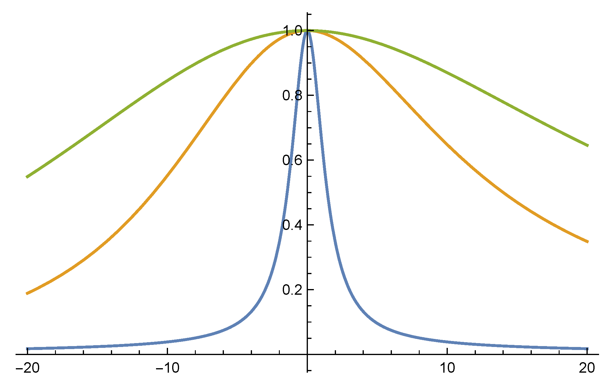
The DOC for the CSD in Equation (5), for , is shift-invariant (it depends on only), while the present one is not. Some examples are shown in Figure 1 for as a function of x with , letting , , .
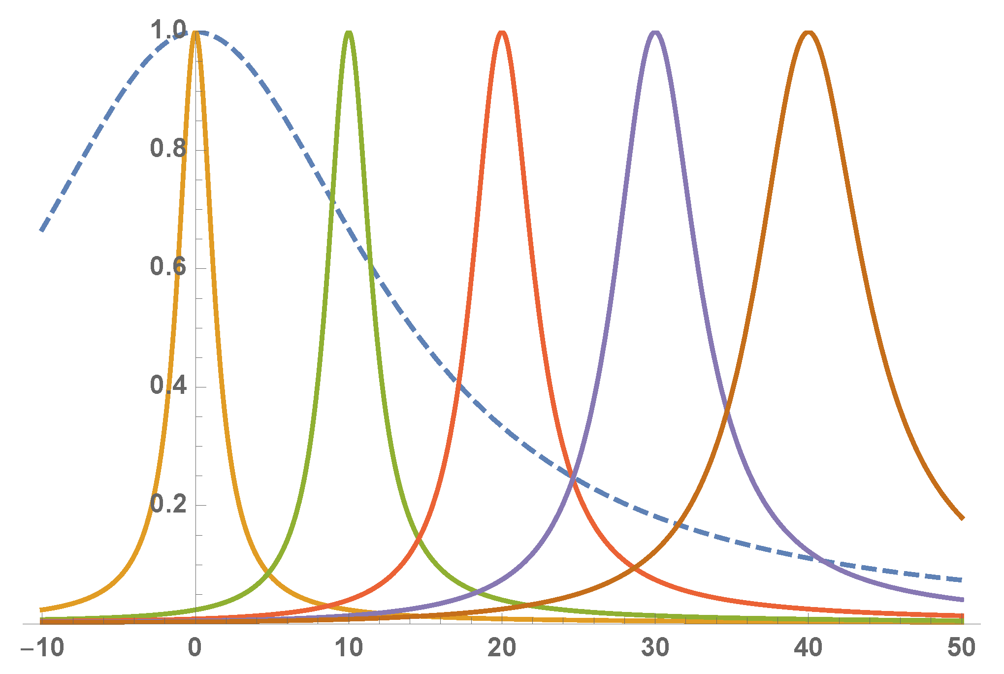
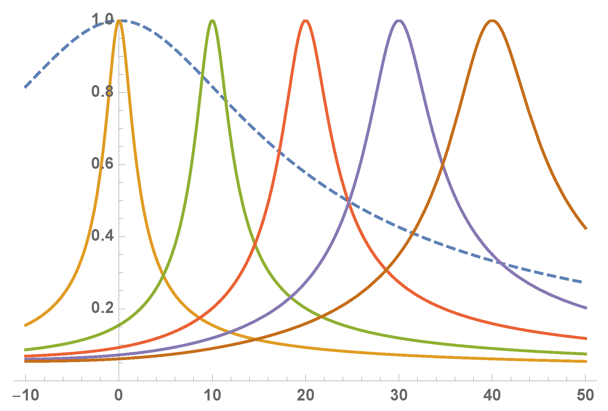
Apparently the field tends to become more and more coherent when grows. Obviously it is important to see whether the growth can occur for appreciable intensities. The answer is affirmative, as confirmed by Figure 2, which shows the curves of the DOC vs. x (with ), for , , , together with the plot of the normalized intensity (dashed curve). It is interesting to note that, from a superposition of GSM CSDs with suitably chosen parameters, a new source has been obtained whose DOC, roughly speaking, seems to be Gaussian, but it is not shift invariant. In this particular example, the coherence area increases on receding from the source center.
A whole set of sources can be evaluated replacing Equation (8) with a generalized version as follows [8]:
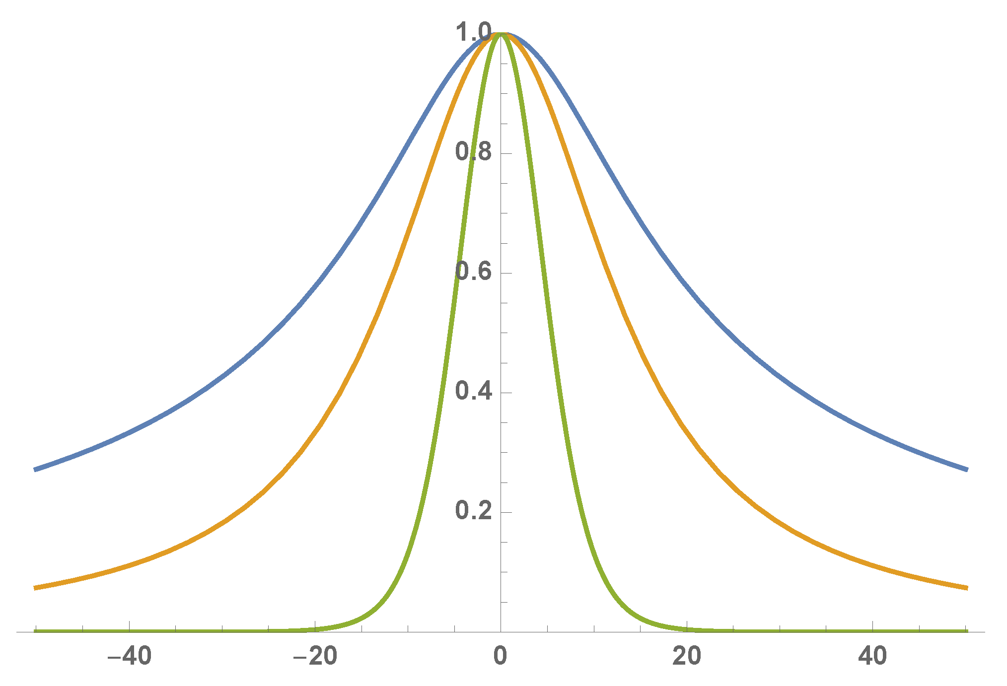
Plots of the normalized intensity are reported in Figure 3 for , , and different values of (0.5, 1, and 5). At first we could think that for increasing only a contraction of the Lorentzian curve occurs. Actually the shape of the curves changes, too. This can be seen on evaluating the abscissa and the I value corresponding to the inflection point where .
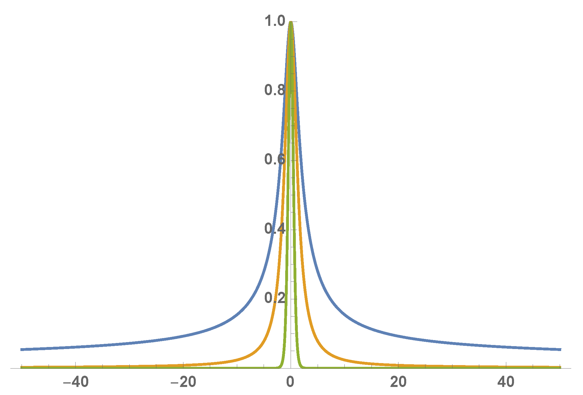
Similar results hold for the DOC. The same values of the parameters have been used in Figure 4 to plot the curves of .
Figure 5 is analogous to Figure 2 and shows the DOC curves as functions of for different values of together with the normalized intensity, with .
Many other examples can be built using a table of Laplace transforms for non-negative functions [8].
3. Shape Invariance
Generally speaking, upon propagation the functional form of the CSDs of the sources in Section 2 will change (see also Section 5). In most cases the propagated field will have to be evaluated numerically. Although the disadvantage of this has been progressively reduced by the availability of more and more powerful mathematical softwares, we may wonder whether this can be avoided.
A significant class of cases in which the propagation process is simple to treat is that of shape-invariant (SI) fields [9]. To discuss this case it will be useful to recall the pertinent propagation formulas. For an elementary GSM CSD they are of the following type [1]:
where the propagation factor and the curvature radius are given by
A typical CSD obtained by superposition of elementary GSM CSDs will be shape-invariant if all of them have the same propagation factor. It is seen instead from Equation (9) that for the typical Laplace-like CSD in the integration process the quantities and are replaced by and . Accordingly, the propagation factor varies with v and there cannot be any shape invariance except when is delta-like.
Yet, a pseudo-Laplace superposition of GSM CSDs with one and the same factor can be generated as follows, leading to our second class of sources. The basic remark is that the propagation factor depends on a specific combination of and ((see Equation (18)). This implies that an infinite number of different couples , can give rise to one and the same propagation factor. In fact, on imposing that the quantity
be constant, Equation (18) takes the form
which is independent of v. Such a choice guarantees that all the constituting beams spread with the same rate upon propagation and give rise, up to a curvature factor and a transverse scaling factor, to the same CSD as that across the starting plane.
It remains to be seen how to choose and . First, for a chosen , the needed value of for obtaining a prescribed K is deduced by
Alternatively, for any chosen , the required value of is obtained by
Note that, since , Equation (21) requires
An elementary example obtained through superposition of only two CSDs will help to appreciate the effects of the superposition. Consider the following CSD structure, where proportionality factors have been omitted:
where the intensity and DOC variances are such that
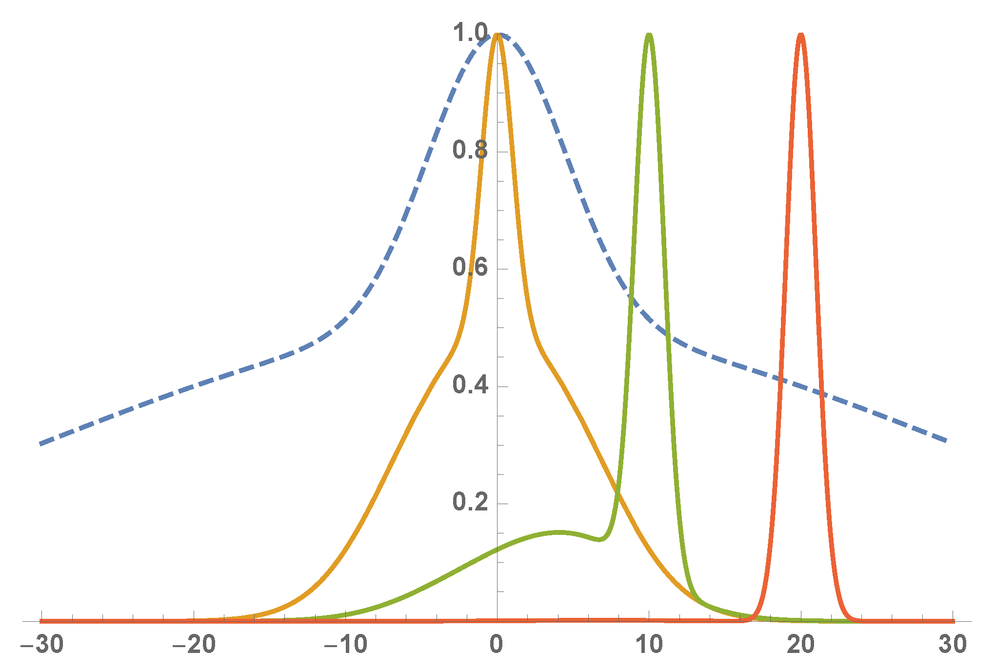
The main effects of the superposition can be appreciated by the curves of Figure 6, drawn for , , , and , the latter being derived from Equation (22). The curve of the normalized intensity (the dashed one) clearly shows the superposition of two Gaussian functions of different width. If the light were coherent the shape of the curve would change on propagation because the initially narrower curve would spread at a higher rate than that of the initially wider curve. A value of z would even exist at which the two contributions would have the same width (even if with different height and curvature radius). With shape-invariant light, instead the intensity profile does not change because the narrower peak is made suitably less coherent than the other. The effect on the DOC is subtler. Within the central region, the DOC curve is not Gaussian (not even approximately), and its shape roughly resembles the intensity profile. Across the lateral wings of the intensity pattern, where essentially only one of the two beams contributes light, the DOC curve is nearly Gaussian, and is narrower than in the central peak.
Let us pass to the general case of shape invariance. What is required is the continuous superposition of GSM CSDs weighted with a function in which the shape-invariance condition is satisfied for any value of v. Thanks to Equation (22), this occurs for
where we put
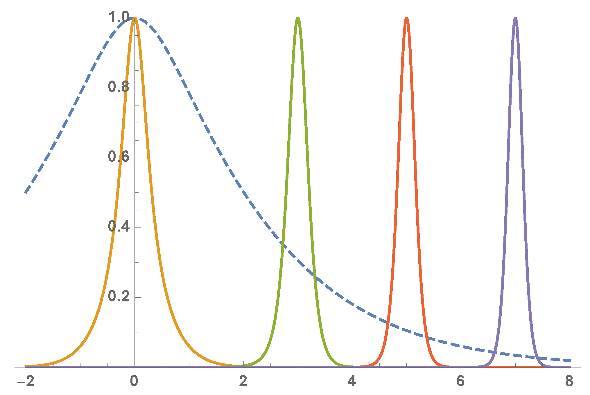
An example is shown in Figure 7, which shows the DOC curves for four different values of , together with the normalized intensity (the widest curve). There we put and the weight function has been chosen as in Equation (8), with . The obtained result is somewhat similar to that shown in Figure 2, but in this case the coherence area decreases on receding from the source center.
4. Modes of Shape-Invariant Sources
As well known, the modal theory of coherence [1] gives a useful tool for the physical interpretation of coherence-depending phenomena and for the study of the propagation of partially coherent fields. It requires the determination of eigenfuctions (the modes of the source) and eigenvalues of the following homogeneous Fredholm integral equation of the second kind [1]:
In this section, we evaluate modes and eigenvalues of the CSD in Equation (26).
According to Mercer’s theorem, the elementary GSM CSD can be expanded in the following series [10]
where
being the n-th Hermite polynomial [8]. Finally is given by
where and are given by Equation (27) and the spot-size is derived from the formula [10]
Since we work with a prescribed value of K, does not depend on v, so that all the elementary sources in the integral (26) have the same modes, and the latter equation can be written as
On inserting from Equation (33) into Equation (2) we obtain the modal expansion of , i.e.,
whose eigenvalues have the form
This is a remarkable property, in that it solves the integral equation in Equation (28) for an infinite class of kernels, which depend on the choice of the positive parameter K and on the form of the nonnegative function .
5. A Condition for Shape Invariance
The shape-invariance property of a CSD is defined with reference to its propagation features [9]. Since the latter are tied to the properties of Hermite–Gauss (HG) modes, we shall say a CSD is SI to mean that it can be expanded in a series of HG modes with non-negative coefficients [11,12,13,14,15,16,17]. Deciding whether a given CSD is SI without knowing its modal expansion could not seem a simple task. Here we show that this can be done using a criterion based on the second order partial derivatives of the CSD.
To simplify the derivation let us rewrite the functions defined in Equation (30) as
where are normalization factors and is the spot size of the modes.
Imagine we have a CSD . Since it is SI, we know it admits of a modal expansion of the form (a real W is assumed)
with non-negative eigenvalues , although we do not know the value of . Now differentiate twice W with respect to and remember the property
derived from Equation 22.6.20 of [8]. The second order partial derivative of W with respect to then reads
where L is the symmetric kernel
Repeating derivation with respect to , we similarly obtain
so that on subtracting Equation (41) from Equation (40) we have
In conclusion, if the CSD W is SI it has to satisfy Equation (42). The condition expressed in Equation (42) provides a tool to ascertain whether a given CSD is of the SI type, by checking its functional features, in that the right-hand side has to be proportional to . Once this is verified, Equation (42) also gives the value of , which was introduced as an unknown in Equation (37).
As an added bonus of the previous derivation we note that, if W is SI, we can generate further genuine SI CSDs by simple differentiation. In fact is shown to be SI by Equation (40) whose closed form expression is obtainable by one of the two following formulas
or, in a more symmetric way, from
This procedure can be repeated iteratively starting from instead of .
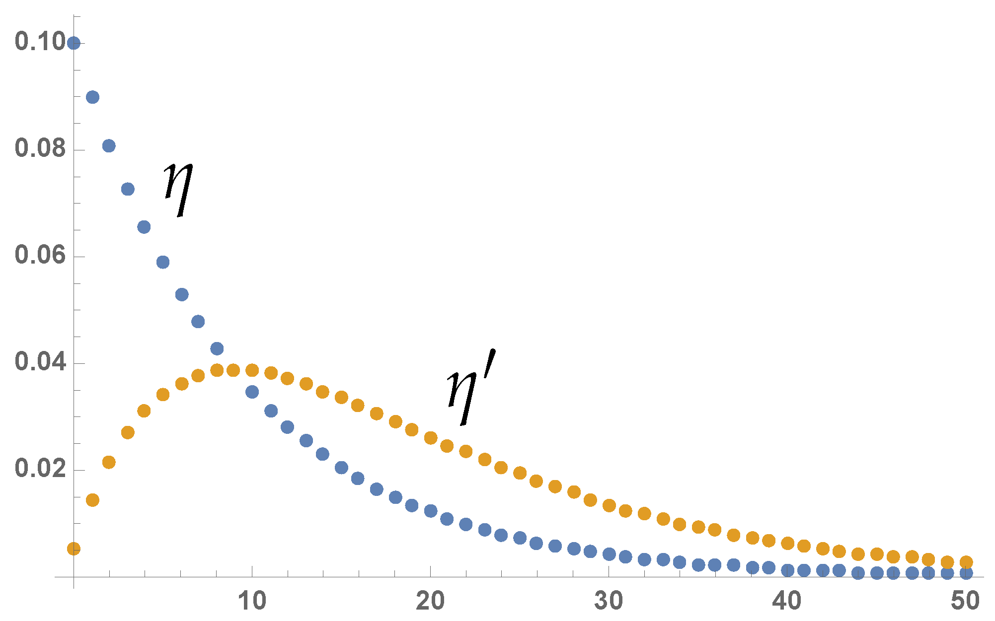
It is to be noted that the eigenvalues of L are significantly modified with respect to those of W. For example, if W is the CSD of a GSM source, its eigenvalues are of the form (see Equation (30))
with and a suitable constant. The eigenvalues of L are
and are considerably depressed for low indices and enhanced afterward. We can normalize them in such a way that for both of them the sum from 0 to ∞ is 1. This requires
The plots of the eigenvalues are shown in Figure 8.
It will be noticed that the differential operator appearing in Equation (38), whose functional structure can be reduced to
is the Hamiltonian of the quantized harmonic oscillator [18]. In this view, Equation (36) specifies the energy eigenfunctions, and the CSD (37) plays the role of the density operator [18]. This formal analogy played a role in recent research about partially coherent sources described by the Christoffel Darboux formula [16] and could be further exploited here.
It can also be noted that from the HG family further sets of orthonormal modes can be derived for propagation in lossless first-order optical systems [19].
6. Conclusions
In this paper, we examined two classes of sources that offer variable coherence features across their area. Both of them are based on the familiar GSM sources, but are endowed with a space variant DOC.
The first approach emphasizes the role that the Laplace transform, with its rich set of properties, may have in the problem at hand.
The second approach examines variant coherence sources in the realm of SI CSDs where the propagation problems become fairly simple. The two basic results are: (a) the solution of the infinite set of involved integral equations and (b) the derivation of a simple differential test to ascertain whether an assigned CSD is SI.
Author Contributions
F.G. and M.S. contributed equally to this work. All authors have read and agreed to the published version of the manuscript.
Funding
This research received no external funding.
Institutional Review Board Statement
Not applicable.
Informed Consent Statement
Not applicable.
Data Availability Statement
Not applicable.
Conflicts of Interest
The authors declare no conflict of interest.
Abbreviations
The following abbreviations are used in this manuscript:
| CSD | cross-spectral density |
| GSM | Gaussian Schell model |
| DOC | degree of coherence |
| SI | shape-invariant |
| HG | Hermite–Gauss |
References
- Mandel, L.; Wolf, E. Optical Coherence and Quantum Optics; Cambridge University Press: Cambridge, UK, 1995. [Google Scholar] [CrossRef]
- Gori, F.; Santarsiero, M. Devising genuine spatial correlation functions. Opt. Lett. 2007, 32, 3531–3533. [Google Scholar] [CrossRef] [PubMed] [Green Version]
- Martínez-Herrero, R.; Mejías, P.M.; Gori, F. Genuine cross-spectral densities and pseudo-modal expansions. Opt. Lett. 2009, 34, 1399–1401. [Google Scholar] [CrossRef] [PubMed]
- Gori, F.; Martínez-Herrero, R. Reproducing Kernel Hilbert spaces for wave optics: Tutorial. J. Opt. Soc. Am. A 2021, 38, 737–748. [Google Scholar] [CrossRef] [PubMed]
- Ping, C.; Liang, C.; Wang, F.; Cai, Y. Radially polarized multi-Gaussian Schell-model beam and its tight focusing properties. Opt. Express 2017, 25, 32475–32490. [Google Scholar] [CrossRef]
- Zhu, X.; Wang, F.; Zhao, C.; Cai, Y.; Ponomarenko, S.A. Experimental realization of dark and antidark diffraction-free beams. Opt. Lett. 2019, 44, 2260–2263. [Google Scholar] [CrossRef] [PubMed]
- Bracewell, R. The Fourier Transform and Its Applications, 3rd ed.; McGraw-Hill: New York, NY, USA, 1999. [Google Scholar]
- Abramowitz, M.; Stegun, I. (Eds.) Handbook of Mathematical Functions; Dover Publications Inc.: Mineola, NY, USA, 1972. [Google Scholar]
- Gori, F. Mode propagation of the field generated by Collett-Wolf Schell-model sources. Opt. Commun. 1983, 46, 149–154. [Google Scholar] [CrossRef]
- Gori, F. Collett-Wolf sources and multimode lasers. Opt. Commun. 1980, 34, 301–305. [Google Scholar] [CrossRef]
- Simon, R.; Sundar, K.; Mukunda, N. Twisted Gaussian Schell-model beams I: Symmetry structure and normal-mode spectrum. J. Opt. Soc. Am. A 1993, 10, 2008–2016. [Google Scholar] [CrossRef]
- Borghi, R.; Santarsiero, M. Modal decomposition of partially coherent flat-topped beams produced by multimode lasers. Opt. Lett. 1998, 23, 313–315. [Google Scholar] [CrossRef] [PubMed]
- Gori, F.; Santarsiero, M.; Borghi, R.; Guattari, G. Intensity-based modal analysis of partially coherent beams with Hermite–Gaussian modes. Opt. Lett. 1998, 23, 989–991. [Google Scholar] [CrossRef] [PubMed] [Green Version]
- Ponomarenko, S.A. A class of partially coherent beams carrying optical vortices. J. Opt. Soc. Am. A 2001, 18, 150–156. [Google Scholar] [CrossRef] [PubMed]
- Koivurova, M.; Ding, C.; Turunen, J.; Pan, L. Partially coherent isodiffracting pulsed beams. Phys. Rev. A 2018, 97, 023825. [Google Scholar] [CrossRef] [Green Version]
- Martínez-Herrero, R.; Gori, F. Christoffel-Darboux sources. Opt. Lett. 2021, 46, 973–976. [Google Scholar] [CrossRef] [PubMed]
- Martínez-Herrero, R.; Santarsiero, M.; Piquero, G.; Gonzáles de Sande, J.C. A New Type of Shape-Invariant Beams with Structured Coherence: Laguerre-Christoffel-Darboux Beams. Photonics 2021, 8, 134. [Google Scholar] [CrossRef]
- Cohen-Tannoudji, C.; Diu, B.; Laloë, F. Quantum Mechanics; Wiley: Hermann, MO, USA, 1977. [Google Scholar]
- Alieva, T.; Bastiaans, M.J. Orthonormal mode sets for two-dimensional fractional Fourier transformation. Opt. Lett. 2007, 32, 1226–1228. [Google Scholar] [CrossRef] [PubMed] [Green Version]
Figure 1.
DOC vs. x with , , , for (from the narrowest to the widest curve).

Figure 2.
DOC vs. x with , for , , (from left to right). The dashed curve is the normalized intensity.
Figure 2.
DOC vs. x with , for , , (from left to right). The dashed curve is the normalized intensity.

Figure 3.
Intensity profiles vs. x given by Equation (15), for , , and (from the widest to the narrowest curve).
Figure 3.
Intensity profiles vs. x given by Equation (15), for , , and (from the widest to the narrowest curve).

Figure 4.
Plots of vs. x given by Equation (16) for , , and (from the widest to the narrowest curve).
Figure 4.
Plots of vs. x given by Equation (16) for , , and (from the widest to the narrowest curve).


Figure 6.
Normalized intensity (dashed curve), together with , and vs. x (from left to right) for the CSD in Equation (24), with , , , and .
Figure 6.
Normalized intensity (dashed curve), together with , and vs. x (from left to right) for the CSD in Equation (24), with , , , and .

Figure 7.
Normalized intensity (dashed curve), and DOC , , , vs. x, from Equations (8) and (26) with and .


Publisher’s Note: MDPI stays neutral with regard to jurisdictional claims in published maps and institutional affiliations. |
© 2021 by the authors. Licensee MDPI, Basel, Switzerland. This article is an open access article distributed under the terms and conditions of the Creative Commons Attribution (CC BY) license (https://creativecommons.org/licenses/by/4.0/).
Share and Cite
MDPI and ACS Style
Gori, F.; Santarsiero, M. Variant-Coherence Gaussian Sources. Photonics 2021, 8, 403. https://doi.org/10.3390/photonics8090403
AMA Style
Gori F, Santarsiero M. Variant-Coherence Gaussian Sources. Photonics. 2021; 8(9):403. https://doi.org/10.3390/photonics8090403
Chicago/Turabian StyleGori, Franco, and Massimo Santarsiero. 2021. "Variant-Coherence Gaussian Sources" Photonics 8, no. 9: 403. https://doi.org/10.3390/photonics8090403
Note that from the first issue of 2016, this journal uses article numbers instead of page numbers. See further details here.