Article

Parametric Mid-Spatial Frequency Surface Error Synthesis

1
Wyant College of Optical Sciences, University of Arizona, 1630 East University Blvd., Tucson, AZ 85721, USA
2
Collins Aerospace, 7 Technology Park Drive, Westford, MA 01866, USA
3
ELE Optics Inc., 405 East Wetmore, #117-260, Tucson, AZ 85705, USA
4
School of Space Research, Kyung Hee University, 1732 Deogyeong-daero, Yongin 17104, Korea
5
Department of Astronomy and Steward Observatory, The University of Arizona, Tucson, AZ 85721, USA
*
Author to whom correspondence should be addressed.
Photonics 2021, 8(12), 584; https://doi.org/10.3390/photonics8120584
Submission received: 15 November 2021 / Revised: 10 December 2021 / Accepted: 14 December 2021 / Published: 16 December 2021
(This article belongs to the Special Issue Advances in Optical Metrology)

Abstract

:
Standard mid-spatial frequency tooling mark errors were parameterized into a series of characteristic features and systematically investigated. Diffraction encircled and ensquared energy radii at the 90% levels from an unpowered optical surface were determined as a function of the root-mean-square surface irregularity, characteristic tooling mark parameters, fold mirror rotation angle, and incident beam f-number. Tooling mark frequencies on the order of 20 cycles per aperture or less were considered. This subset encompasses small footprints on single-point diamond turned optics or large footprints on sub-aperture tool polished optics. Of the characteristic features, off-axis fabrication distance held the highest impact to encircled and ensquared energy radii. The transverse oscillation of a tooling path was found to be the second highest contributor. Both impacts increased with radial tooling mark frequency.

1. Introduction

Tooling marks (TM) refer to unwanted errors in the surface figure of an optic, which are a byproduct of the means of fabrication. The nature of standard fabrication techniques such as single-point diamond turning (SPDT) and sub-aperture tool polishing (SATP) leads to a meaningful subset of these marks being periodic with well-defined forms [1].
The performance implications of some forms of these mid-spatial frequency (MSF) TM are thoroughly described through a variety of analytical techniques, including but not limited to Fourier decomposition of the surface profile [2,3,4,5], analysis of power spectral density (PSD) based on the tool influence function and path [6,7], anisotropic error representation via polar root-mean-square (RMS) surface figure plotting [8], and surface fitting of MSF errors via Q-polynomials [9].
However, the resultant optical performance impacts are fairly limited in their scope. A general case categorization of TMs has yet to be created, yet this systematic case categorization is essential. Frequently optical surface TMs may deviate from previously modelled results. Existing methods consider only specific subsets of TM forms.
There exist standards to quantify the uncertainty between the measured and modelled data [10,11,12]. These approaches allow for thresholds to be determined for allowable deviation of a tooling shape from a specific TM form assumed for these rigorous models. However, the rigorous analytical methods would need to be repeated in order to quantify this uncertainty for each initial case. Furthermore, the parameters driving these additional TM subsets require additional definition.
This paper consolidates and categorizes typical TM characteristics observed across SPDT and SATP. It then defines a set of input variables to control specifics of the resultant tooling profile. These inputs are then simulated to achieve a parametric optical model to describe diffraction encircled and ensquared spot radii. From this point, standard uncertainty definitions could then be applied.

2. Materials and Methods

In order to understand the impact of TMs, it is first important to understand ways in which TMs can manifest. Different fabrication methods can result in unique residual TM profiles on the final optical surface. The primary fabrications to be explored are single-point diamond turning and sub-aperture tool polishing. The TMs from these fabrication methods share several distinct similarities. This permits for a simultaneous description of both under a single parametric model.

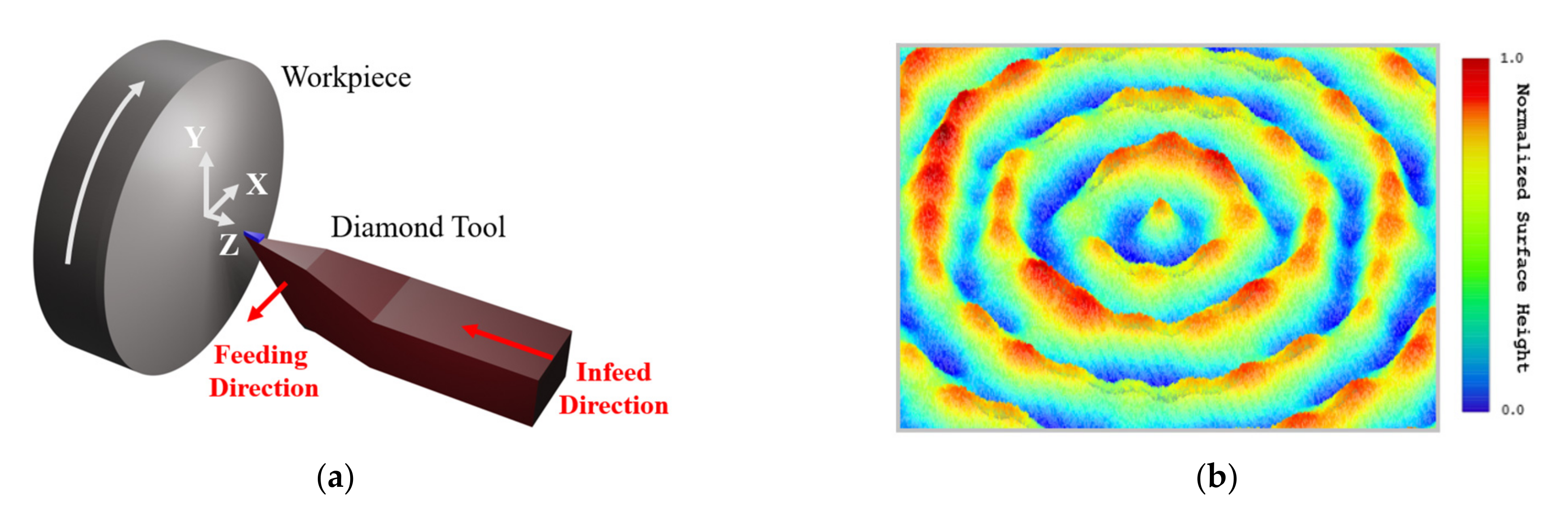
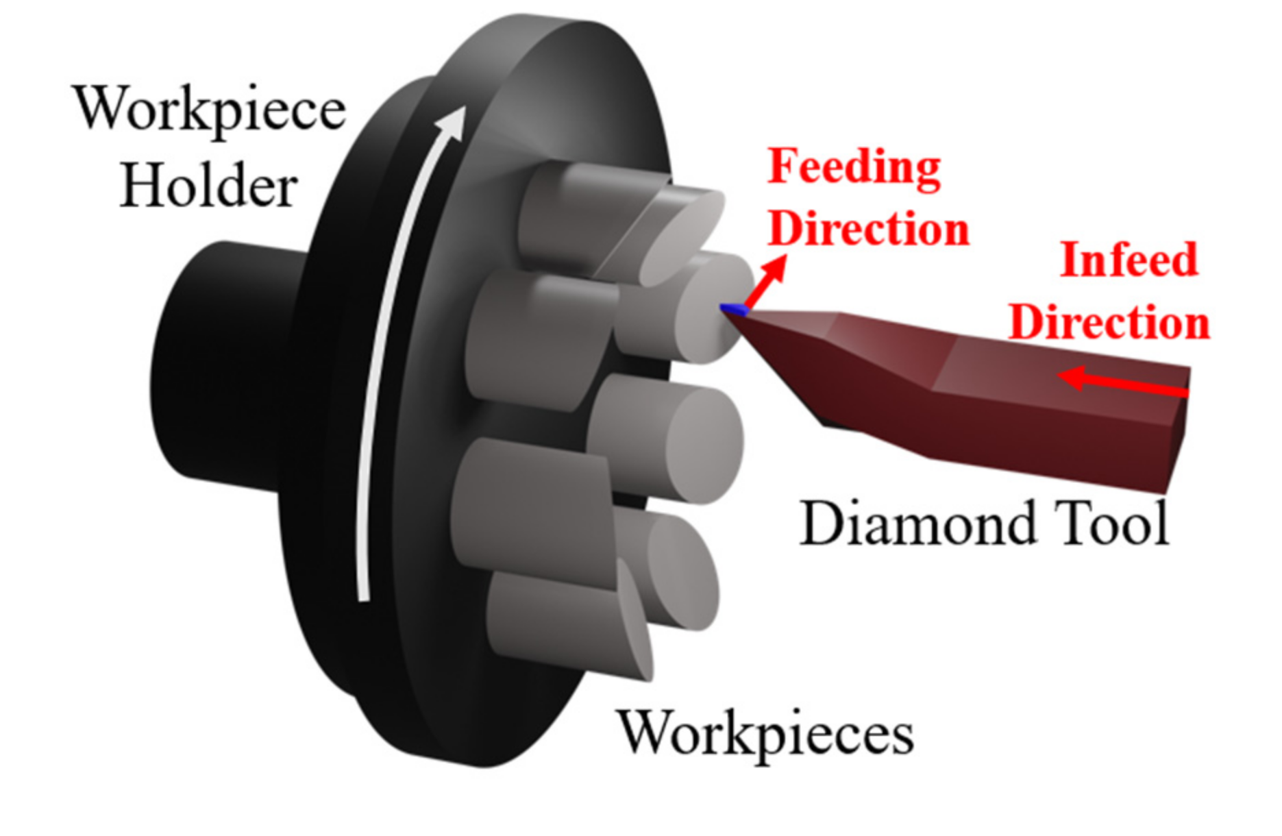
2.1. Single-Point Diamond Turning

SPDT is a manufacturing process that removes material from an optical blank by use of precision lathes (or equivalent rotary machine tooling) equipped with a diamond-tipped tooling bit. This process is used for a wide array of optics from optical flats to freeform surfaces [1].
The optical blank is fastened to the rotary plate and spun at high speeds. During this rotary motion, the diamond-tipped tooling bit contacts the surface to remove material along a given path. This process is repeated in predefined patterns such that material is removed across the substrate. This process proceeds until the final surface profile is achieved in compliance with the optical specifications. Micro-roughness of approximately 5 nm RMS or less is achievable with SPDT [1,13]. Lower micro-roughness is achievable via post-processing operations such as magnetorheological finishing (MRF). However, this increases the processing time and drives up the cost for the finished part. Figure 1 demonstrates the SPDT process.
The nature of this process yields circular marks along a given tooling track. The exact manifestation in terms of depth, spacing, and overall profile can vary depending on the machining setup and optic under fabrication [14,15]. Other factors such as undamped environmental vibration and thermal expansion of the part/tooling can also impact the profile and magnitude of these marks.
Given the size of the diamond tip, TMs from SPDT are typically very finely spaced relative to size of the optical footprint in a given system. This gives way to diffractive effects because of the fine periodic structures. For footprints at various positions from the optical axis, these effects manifest as varying degrees of the point spread function splitting [16].
The application under investigation in this paper includes mid-spatial frequency TMs, especially, in the regime of 5–20 cycles per aperture (cy/ap). Given the nature of SPDT, this regime encompasses applications in which the mirror is used with a relatively small optical footprint. For example, with a reasonable tool nose radius of 1 mm the frequency regime mentioned would encompass optical footprints between 5 mm and 20 mm in diameter [16]. Given this definition, the analysis range will not extend to larger diamond-turned optics. For the case of larger optics, standard turning tool tip radii would produce TM frequencies outside the frequency regime previously mentioned.

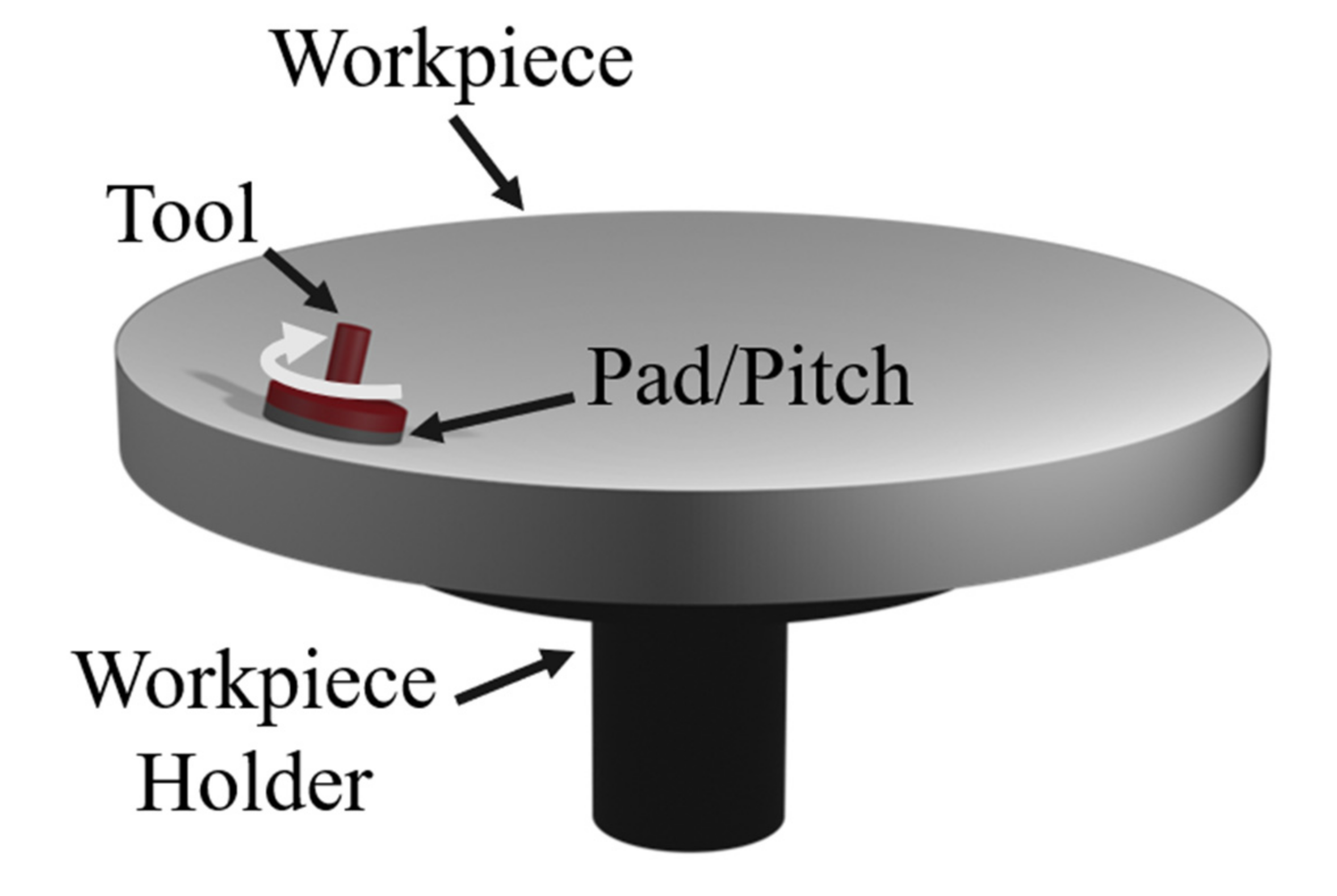
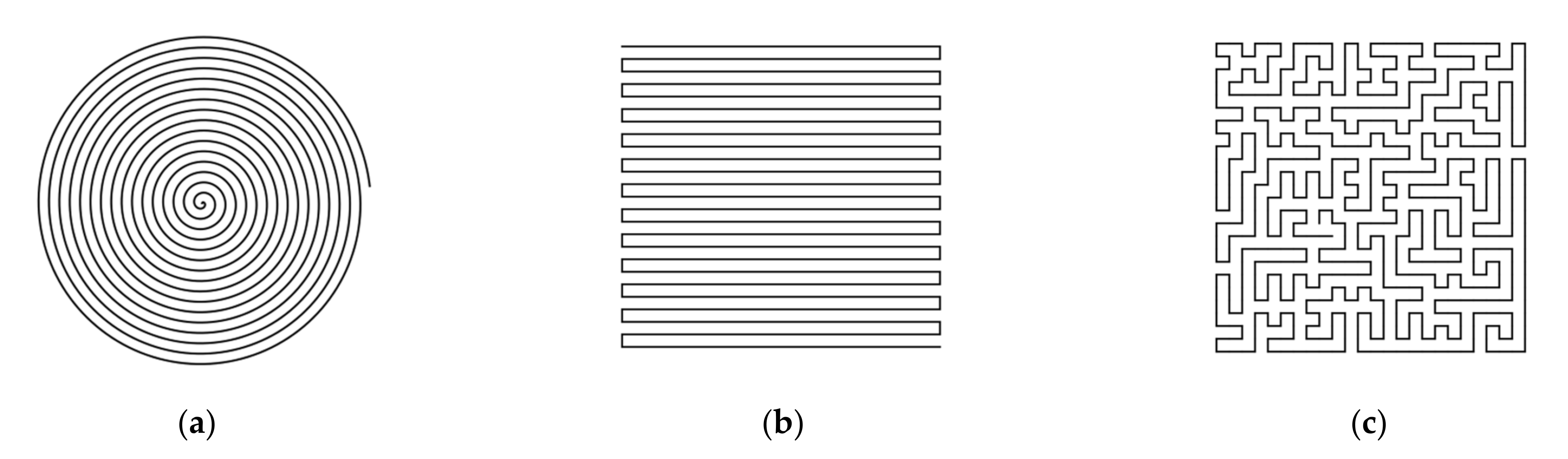
2.2. Sub-Aperture Tool Polishing

SATP is a technique in which a tool undersized compared to the diameter of the workpiece is rotated and scanned across the optical surface using an abrasive polishing compound to remove material. Figure 2 shows the general setup for the SATP process, which is often called Computer Controlled Optical Surfacing [17].
There are a multiple of tool paths that can be employed depending on the application including Archimedes “spiral” paths, raster scanning “zig-zag” paths, and pseudo-random “algorithmic” paths [7]. These paths are demonstrated in Figure 3.
The result of each path is a distinct set of TMs that form the MSF regime for most optics. For this analysis, the raster scanning and Archimedes-type paths will be considered. The pseudo-random path is omitted from this analysis due to the direct dependence on the particular path generation algorithm selected [18,19]. This would lend a parametric model to be specific to a single algorithm rather than a more generalized formulation as is being explored.
Unlike diamond turning where the residual error is found to be relatively high frequency across the part, the tooling residual error of sub-aperture tool polishing has a large range of MSF errors across a given aperture. This range is dictated by the tool path, the tool size selection, as well as the size of the part under fabrication. For this paper, tooling frequencies on the order of approximately 20 cycles per aperture or less are considered.
It is worth noting that the spacing and scale of TMs from SATP are physically much larger than those resulting from SPDT. This is due to the specific mechanisms that create each set of TMs. The main scope of this numerical simulation study is to focus on the optical performance impacts across various classes of mid-spatial frequency errors regardless of their specific origin. In practice, the surface error of a given part is the combination of various manufacturing processes such as generating, grinding, optical mounting for fabrication, post processing, etc.
Additionally, the surface error scale can be a strong function of optical system’s wavelength (e.g., Extreme Ultraviolet lithography system vs. Terahertz space telescope) and the aperture size (e.g., a 1 mm aperture diameter lens for an endoscope vs. an 8 m aperture diameter mirror for an astronomical telescope). The simulation to be presented does not account for diffraction effects at the surface interface such as with high order degradations due to the fine scale of high spatial frequency errors. However, the diffractive effects of propagation are otherwise considered. This paper limits the scope of analysis to features that produce a spot size greater than the diffraction limited spot size. After defining the critical TM parameters in Section 3, and describing the parametric modelling approach in Section 4, the limits of each parameters will be discussed in Section 5.

3. Classification of Tooling Mark Features

To describe the anticipated surface errors imposed by various forms of TMs, the contributions are decomposed into a pair of terms as shown in Equation (1).
F s u r f = G ρ + H z ,
The first term, Gρ, represents the traditional TM definition of periodic oscillation across the aperture. This term includes a radially symmetric base term alongside a sub-term that dictates an along-track oscillation. The subscripts of radial distance ρ is meant to emphasize the primarily oscillation modes of this term. The second term, Hz, represents a periodic depth variation along a given TM track. Here, the subscript of height from the surface z is meant to emphasize the out-of-plane nature of this term. The terms Gρ and Hz will be expanded upon in Equations (2) and (4).
Several variants of TMs will be explored, which can be described by this parametric description. For consistency, spatial terms described in this paper, such as the surface heights described by these characteristic terms, will maintain units of micrometers. The most common TMs will be referred to in this paper as radial TMs. These are demonstrated in Figure 4 and are the result of rotationally symmetric tooling error fabricated into the surface of the part. From these, several sub-classes will be broken out and described including in-plane TMs, out-of-plane TMs, and off-axis TMs.
The three radial subclasses are all a result of breaking rotational symmetry. The distinction between each subclass comes in the way in which this rotational symmetry is broken. In-plane TMs describe variation of a given TM track parallel to the surface plane. Out-of-plane describes a similar but orthogonal implementation in which the depth of the marks is variable with position along a tooling track. Off-axis TMs will describe the manifestation of these marks where the centermost TM track is not centered on the aperture of the part (e.g., off-axis parabola manufacturing case).

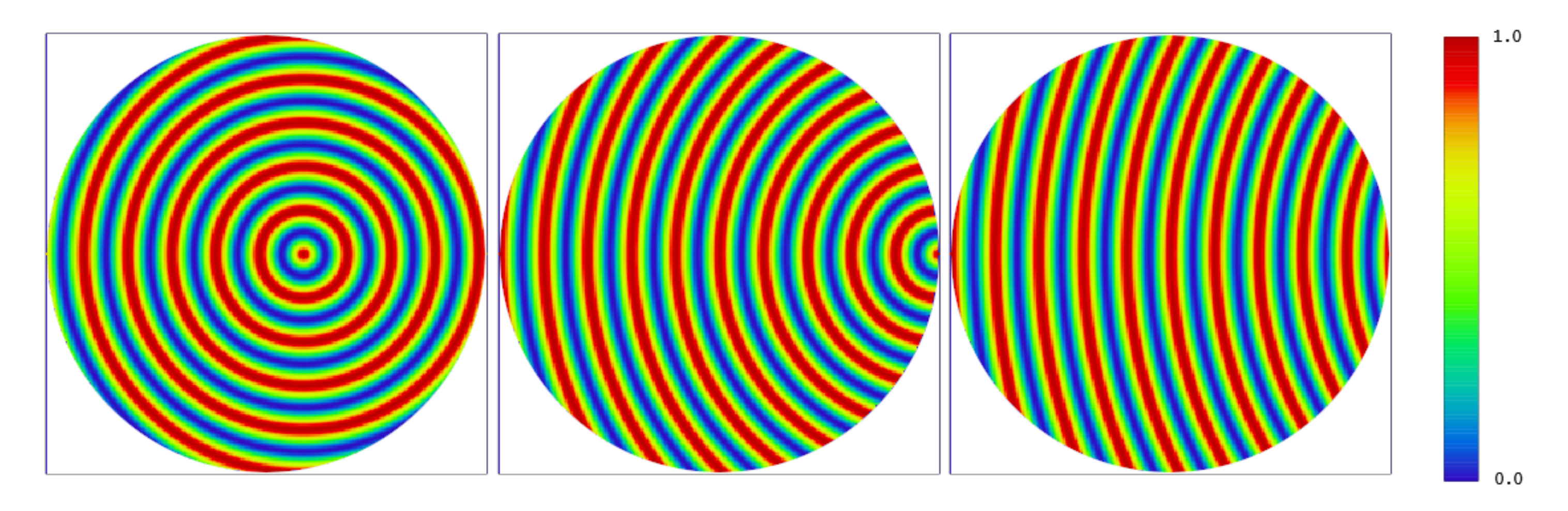
3.1. Radial Rooling Marks, Gρ

Traditional on-axis TMs are described by a radially symmetric oscillation of a given frequency. The process of diamond turning can leave these MSF features present on a completed part. These features can be minimized by post-processing routines, but these are not always mandated by the specifications of a given part. This can be due to the additional processing time this routine adds, thereby potentially increasing the cost of each part. This radial pattern is additionally employed to approximate the Archimedes-type pattern found in SATP as demonstrated in Figure 4a.
For this paper, these features will be approximated as sinusoidal oscillations across a given aperture of diameter DUUT. The functional definition of these oscillations is presented in Equation (2) and Table 1. This is similar to the approximation employed by Rogers in his study of slope error tolerances related to TM phenomena [20] and backed by the results of Liang in the performance impact demonstrated between cusp-type and sinusoid-type groove structures [3]. The associated frequency of these oscillations, ξ, is defined as the number of cyclic oscillations over the given aperture [cy/ap].
G ρ = A cos 2 ξ π D U U T ρ + G φ + 1 ,
The radial coordinate ρ is defined here in addition to an amplitude control variable A. The value of this parameter was used to achieve a specified RMS surface figure error. While the magnitude of the amplitude is trivially derived for a single sinusoidal case, the complexity of this derivation quickly rises with additional characteristic terms. In the implementation for this paper, each profile was scaled according to its as-generated RMS surface figure. The Gφ term represents the contributions from orthogonal oscillations, which will be referred to as in-plane TM. The subscript is meant to emphasize dependence of these oscillations on azimuthal angle φ. Pure radial tooling marks are represented as Gφ goes to 0. This term will be expanded upon in Equation (3).

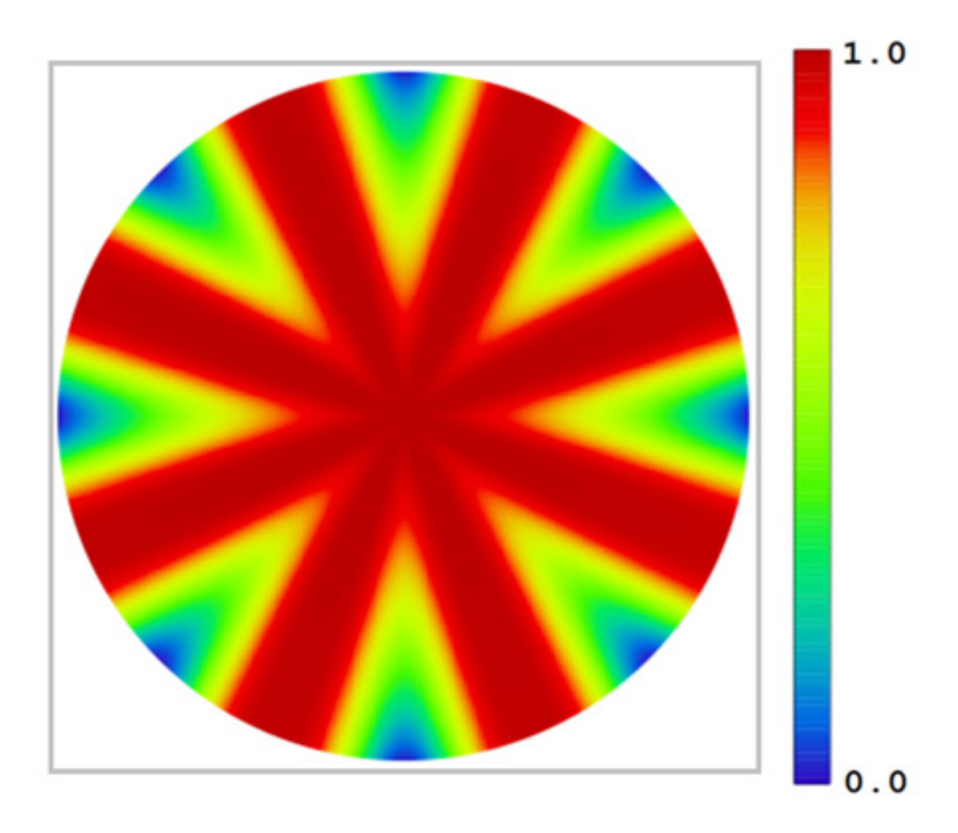
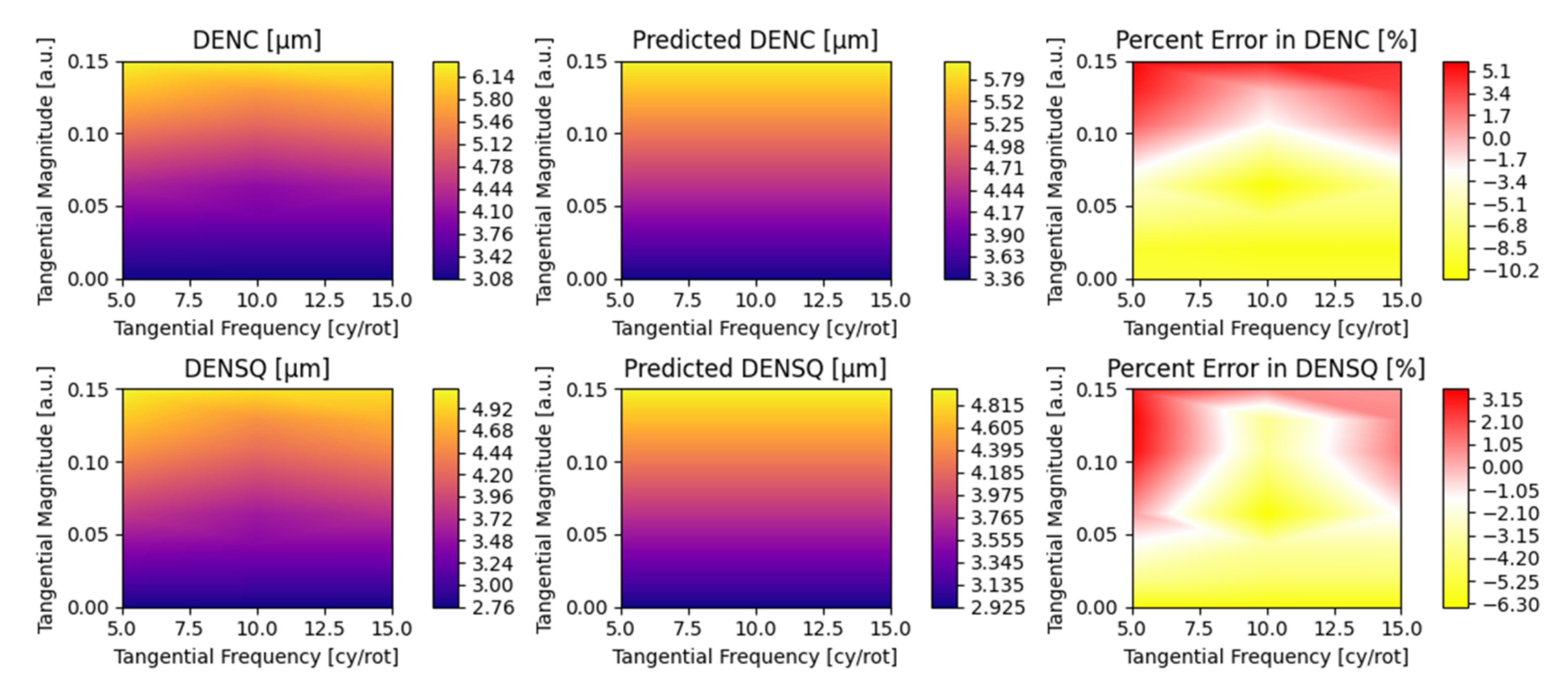
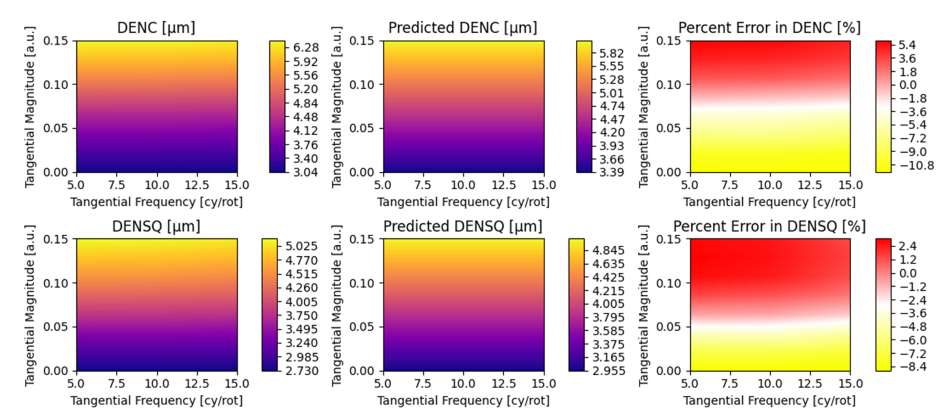
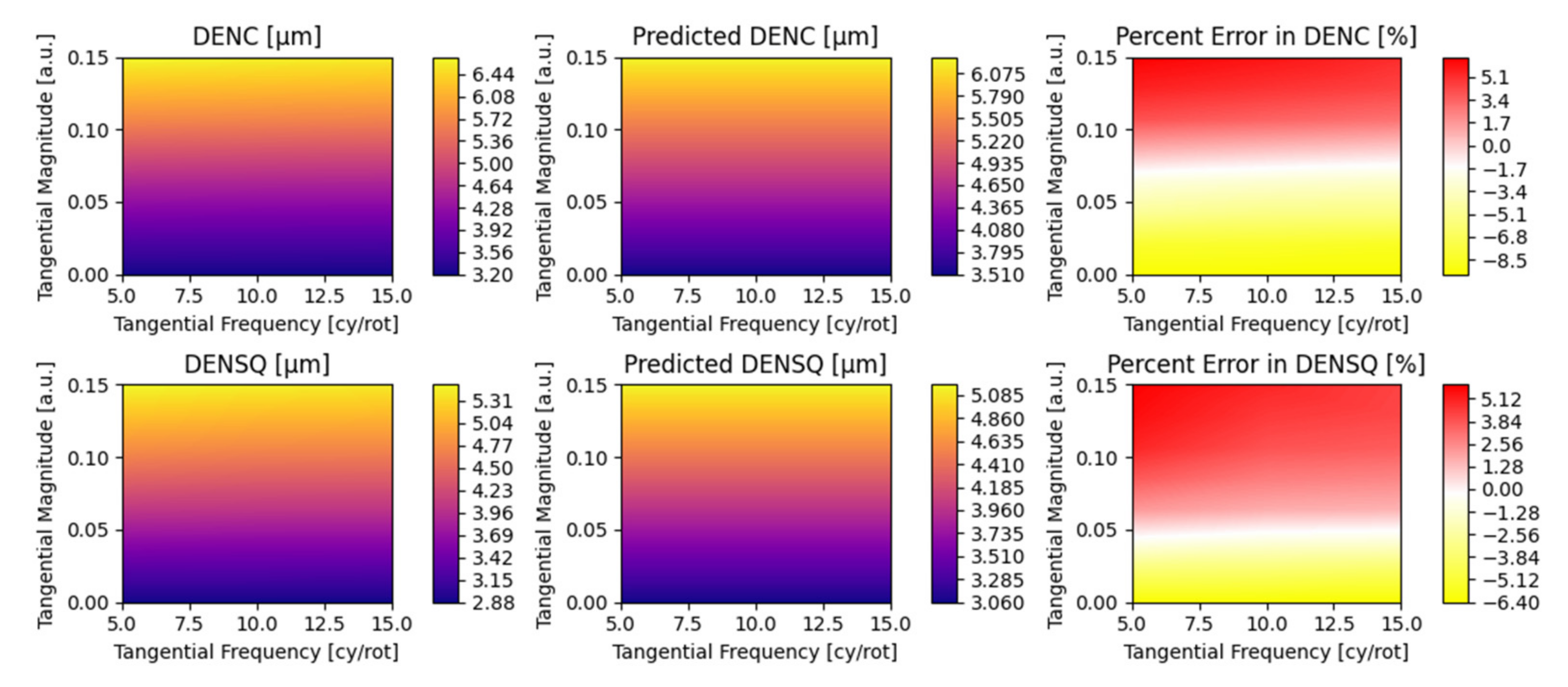
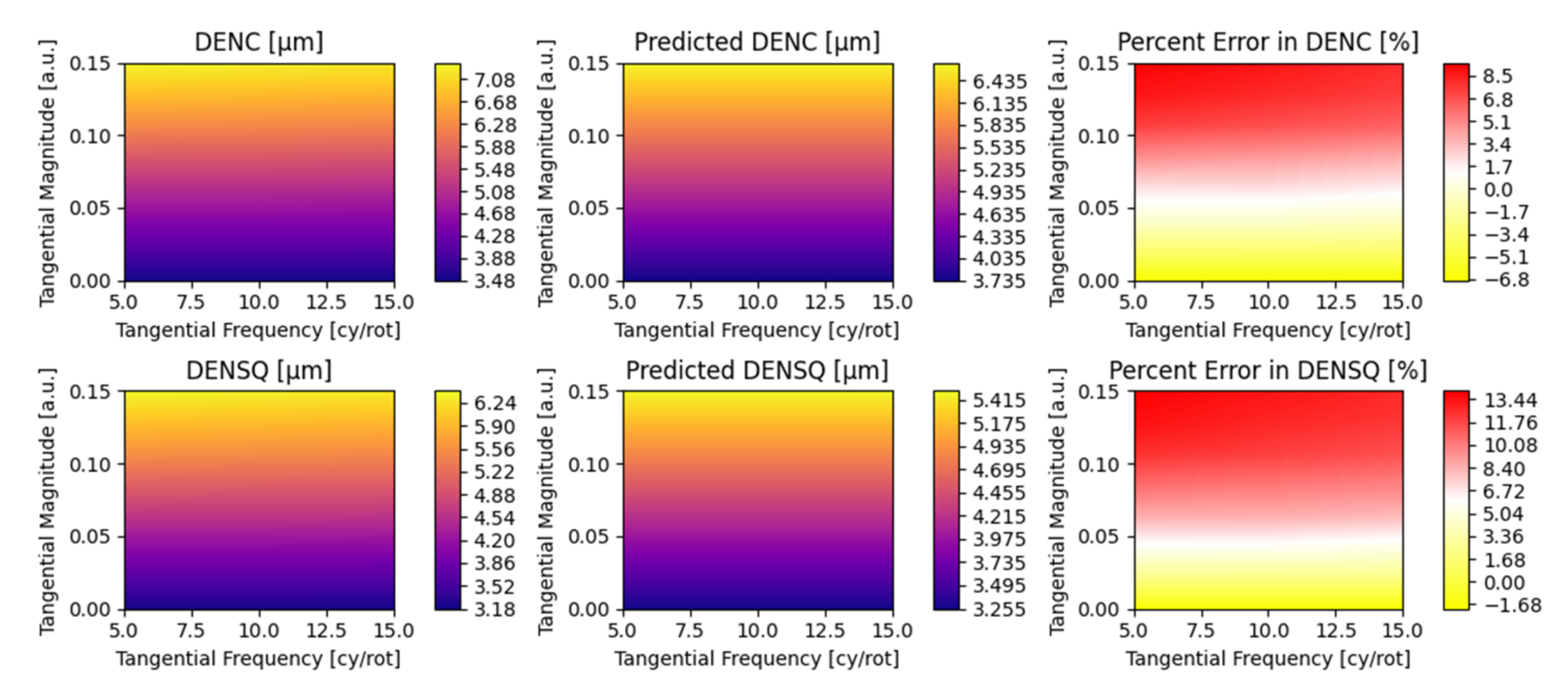
3.2. In-Plane Tooling Marks, Gφ

While radial TMs dictate the variation over a given rotation of the part or tool used for material removal, they are represented as perfectly concentric. In practice TMs do not manifest this concentricity perfectly. Changes including environmental vibration, ambient thermal fluctuation, and thermal fluctuation of the tooling removing material can cause these marks to stray from their ideal path. The case of a primary driving frequency will be considered.
For SATP, the case of constant linear tool speed was considered along a circular path. Due to this, the tangential frequency in units of cycles per rotation increases proportionally with radial distance. It follows that this “seed” frequency parameter relates to the rate of increase with radial distance rather than a constant dependent only on polar angle. Figure 4b demonstrates this effect when overlaid with a base radial TM pattern.
For the case of a singular primary frequency contributor, an equivalent sagittal and tangential frequency are overlaid to approximate the desired spatial effect defined in Equation (3) and Table 2.
G φ κ cos π ω x cos π ω y ,
In this expression, ω refers to the seed tangential frequency parameter that increases with radial position as described prior. The tangential magnitude κ relates to the percentage of which the TM track is perturbed into the next track over with units of length [ap].

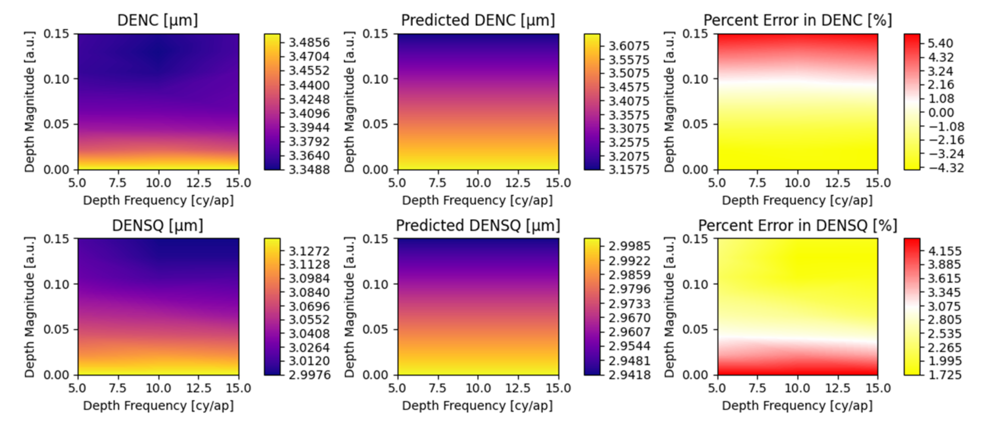
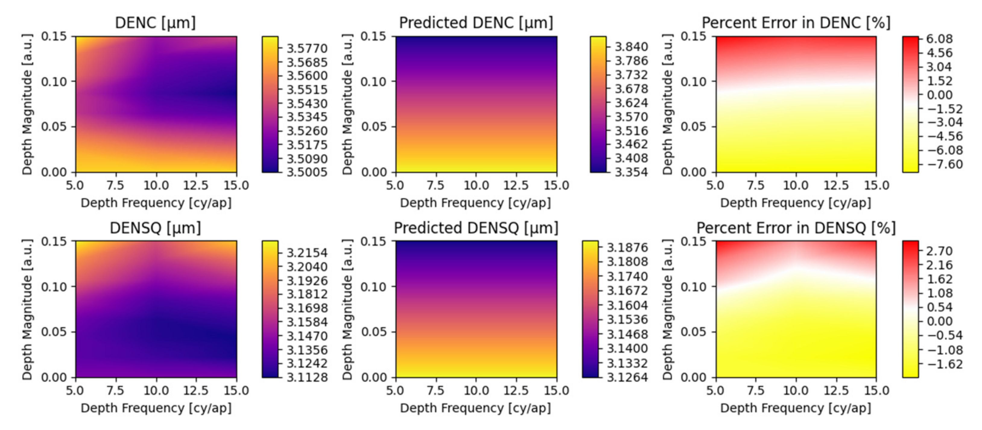
3.3. Out-of-Plane Tooling Marks, Hz

In-plane TMs represent an oscillation within a given TM track, but they do not account for any additional variation in depth over the course of the fabrication. For instance, this change in depth can manifest due to a lack of uniform tool pressure along a given tooling track during a SATP routine. To describe this depth variation, an additional term (Hz) in Equation (1) is summed on top of the traditional radial tooling pattern. These variations will be referred to as out-of-plane TMs and are described by Equation (4) and Table 3. These marks are shown overlaid with a base radial TM pattern in Figure 4c.
Similar to the approach described for tangential TMs, a single out-of-plane TM contribution can be described in terms of a depth magnitude η with an associated depth seed frequency parameter ζ.
H z η cos 2 ζ π D U U T x cos 2 ζ π D U U T y ,
This approach again mimics a constant linear tool speed rather than a constant angular tool speed, so it is typically better suited to model the residual error from a technique such as SATP. As radial distance increases so does the frequency of these depth variations. The rate at which this frequency increases is again dictated by the seed frequency parameter.
A similar manifestation of this error with constant angular frequency instead of constant linear frequency can be found in diamond turning. Specifically, the error can be caused by spindle movement during the turning process. This is referred to in the literature as “spindle star error” [21,22]. It is typically observed for on-axis fabrication in close proximity to the rotation axis. A demonstration of this error can be seen in Figure 5, where the bottom right surface overview shows the gradual falloff with distance from the rotation axis. Spindle star error is a feature of which performance impact is an opportunity for exploration in future work.

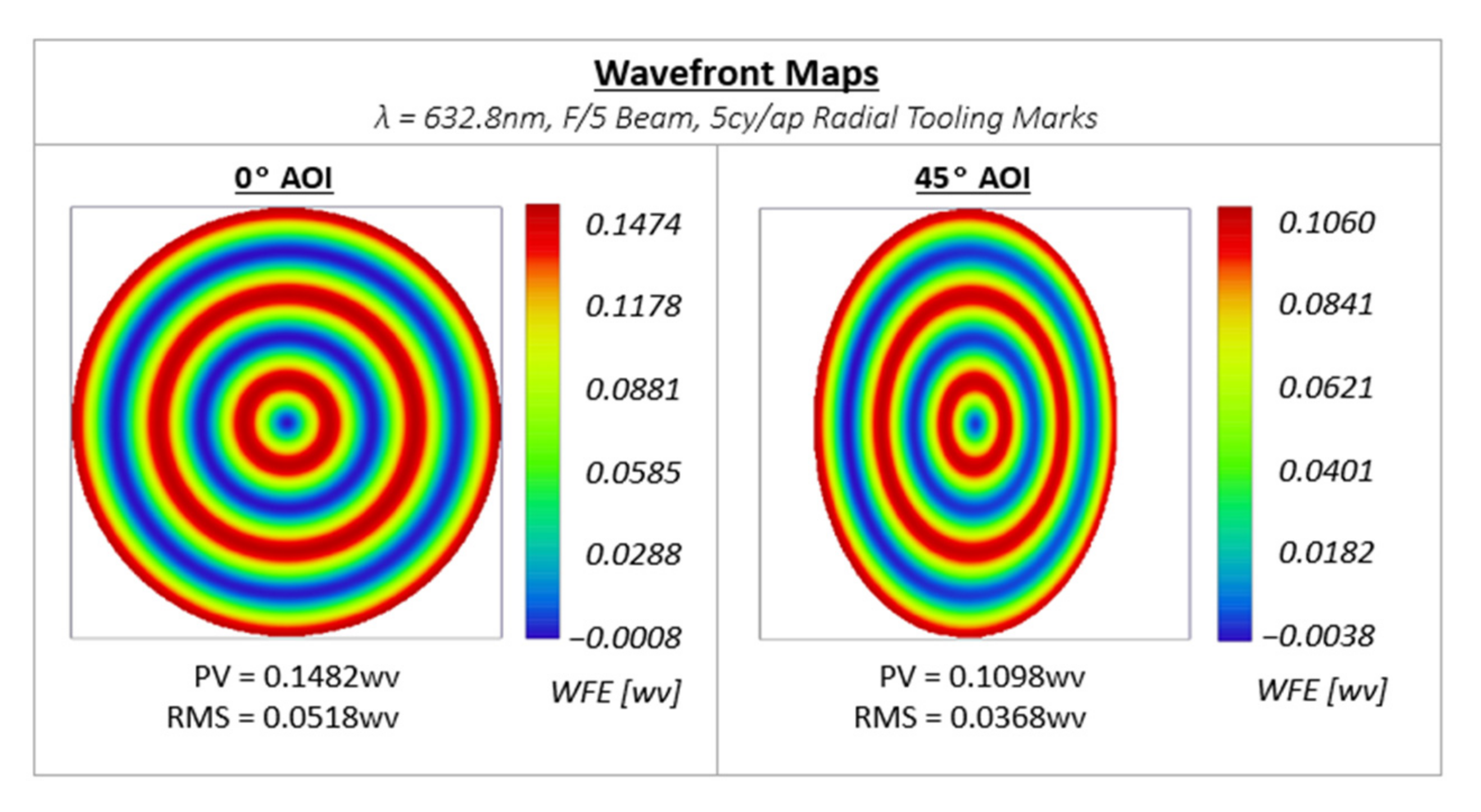
3.4. Off-Axis Radial Tooling Marks

During the process of diamond turning, it is typical to manufacture multiple flats or powered elements simultaneously using a single large spindle. This can either be done with discrete substrates laid out about the rotation axis, as seen in Figure 6 or by fabrication of a larger parent optic from which smaller child optics are drilled [23,24].
These approaches can lead to non-rotationally symmetric TMs shown in Figure 7. The defects resulting from these processes will be referred to as off-axis TMs.
The result of this is a periodic shape with the same TM spatial frequency along the axis of decenter but a lower spatial frequency across the orthogonal axis. At higher decenter positions, the spatial frequency along the orthogonal axis tends towards zero resulting in straight TMs.
These regions are selected by varying the output window for a given surface profile prior to applying the circular aperture mask. Alternatively, the surface region to be analyzed can be kept fixed and the coordinate system altered to achieve the desired surface portion as described in Equation (5) and Table 4. This is achieved by substituting the x and y cartesian spatial coordinates of Equation (3) with (x − Δx) and (y − Δy) for decenter parameters Δx and Δy.
ρ Δ = x Δ x 2 + y Δ y 2 ,

4. Parametric Optical Modelling and Evaluation Criteria

Each of the tooling mark profiles described in Section 3, and more generally each parameter within each tooling mark profile, will have a unique impact to optical performance. However, other more general measurement characteristics will have an impact on this performance as well. These are explored in Section 4.1 such that a model is set up in Section 4.2 to evaluate performance impact for a given collection of parameters. This model is used as a baseline in order to develop a parametric model in Section 5, which allows for more accessible prediction and evaluation of performance impact.

4.1. Optical Model Parametrization

To parametrically predict the performance impact of a composite set of TM features, critical dependencies on test conditions and surface features must be identified and isolated. In addition to the frequency and magnitude parameters for each individual characteristic mark, there are several other parameters (Table 5) that hold high importance in the performance prediction routine.
For the modeling of these composite TMs, the magnitude of the overall surface profile was driven by a given RMS surface irregularity specification. Given the various geometries of the TMs being overlaid, the surfaces were first generated with an approximate PV depth variation magnitude. After generation, an aperture mask was overlaid on the data and the RMS irregularity calculated over the resultant surface. At that stage, the magnitude of depth variation was scaled in order to achieve the desired RMS surface irregularity across the part.
The effect of TMs on a given optical flat at normal incidence may be significant for certain applications such as a return flat in some interferometric measurement setups. However, many imaging applications require the optical flat to be folded at an angle in order to propagate the beam along the desired path.
A variable angle of incidence (AOI) has implications to both the scattering effect of the TMs as well as the projected size of the aperture itself. It also has direct implications to the RMS WFE measured for the reflected wavefront. This leaves the AOI as a critical variable to consider when predicting the performance impact. This is demonstrated in Figure 8 and Figure 9, where the same surface was considered at both normal incidence and 45° incidence.
The diffraction limited case changes due to the outer diameter of the test optic being used as the system pupil. The reason for this choice is to directly represent the performance impact resulting from a footprint across the whole optic. Similarly, the projected size of the pupil results in a lower RMS wavefront being evaluated as well as a lower difference between the diffraction limited and test surface 90% encircled energy levels.
The argument for inclusion of the incident beam f-number is similar to that for AOI. This parameter is critical to consider due to the wide array of use cases and the dependence resulting from the scattering profile. In this context, the diffraction encircled energy radius is directly proportional to the f-number
The metrics investigated are strictly with respect to reflective elements. Calculations are made using a diffractive-inclusive calculation of fraction of encircled energy. Given this, there is a direct linear dependence on wavelength. This dependence can be backed into the parametric results after evaluation at the original analysis wavelength (632.8 nm).
The parametric model is currently only applicable for nominally flat optical surfaces. Radius of curvature, conic form, or other surface attributes are areas for future exploration and implementation.

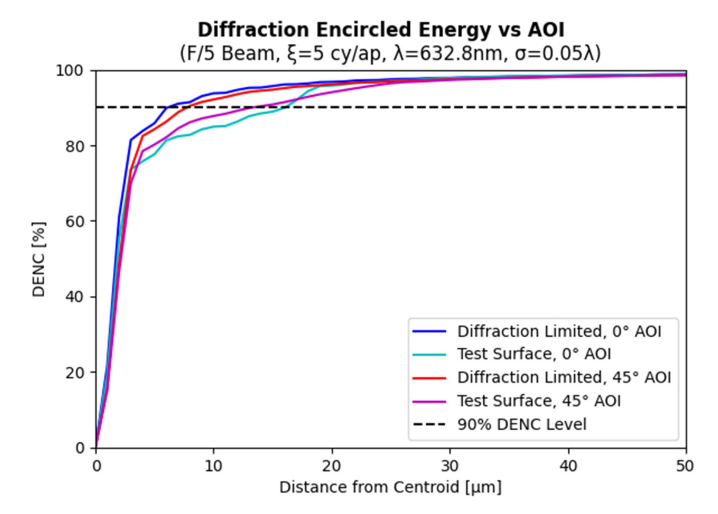
4.2. Performance Metric Calculation Approach

For each TM feature set described in Section 3, alongside each parameter identified in Section 4.1, performance data was generated in order to quantify anticipated performance impact. The performance metric selected was the diffraction encircled energy radius (DENC) and diffraction ensquared energy extent (DENSQ). Specifically, these values were calculated at which the fraction of encircled and ensquared energy was at a level of 90%.
These performance characteristics were calculated using the FFT-based method provided by Zemax OpticStudio 20.2.2. The analysis operations were performed via OpticStudio’s Dynamic Data Exchange interface and metrics exported for external processing.
The optical model of Table 6 was set up to represent a converging beam of variable f-number. This beam reflects from the surface under investigation at a variable AOI. The surface profiles were generated as grid sag surfaces representing physical depth deviation across the part. These profiles were then attached to the mirror surface, which also served as the pupil for the demonstrative system.
Each profile was generated with a sampling frequency of 0.00197 points per mm (0.05 points/inch). This sampling was performed over an aperture of 457.2 mm (18 inches) yielding 360 points across the diameter of the mirror. It was determined that halving the sample frequency from this point yielded negligible difference on the output parameters to be on track.

5. Parametric Regression Optical Performance Synthesis

A parametric model was fit to the dataset for each applicable input term. The goal of this model was to enable simplified approximation of an arbitrary composition of TM features overlaid together to represent a given part, or expected part based on a set of historical fabrication data.
Fitting methodology entailed manual observation of the cross-relationships between each variable. This was used to set up a baseline model and generate first-pass parametric coefficient estimates. These relationships are explored in Section 5.1. A global optimization was then run over the parameter space by a differential evolution algorithm with RMS fit error as the driving metric.
After determining the optimized solution, these parameters were cross-examined through use of a non-linear least squares fit algorithm. The coefficients from the global optimization routine were used as initial conditions for this second verification in order to finely probe the local solution space. The residual error of this fit is further explored in Section 5.2.

5.1. Form of Parametric Fits

Each metric (DENC and DENSQ) retains the same functional form shown in Equation (6). What differs in the description of each metric is the parametric coefficients defined within each of the sub-terms. These parametric coefficients will be denoted with a subscript.
In terms of the overall fit profile, the σ variable represents the RMS surface figure error in units of μm. The θ variable provides upfront scaling for the rotation of the unit under test with respect to the incident cone gut ray angle. The 0.3 term was fit against the as-generated data to track the slight non-linear falloff associated with angles out to 45°. All other variables immediately present relate to the parametric fit of each TM input and cross-term.
F c h a r = σ f # cos 0.3 θ B + κ M + η N + E ,
The default form for Fchar represents the spatial extent for DENC or DENSQ, for a converging beam of a given f-number (f#), in units of micrometers. As described in Section 4.1, the default output assumes an analysis wavelength of 632.8 nm. The result can be scaled by the following linear relationship:
F c h a r , λ 2 = F c h a r + χ ( λ 2 0.6328 μ m ) ,
In this definition, χ is the linear scaling constant related to the metric in question (DENC or DENSQ). Direct wavelength scaling is valid until approximately ~800 nm, after which diffraction effects begin to overshadow the TMs over the regime analyzed. Going down to lower wavelengths (~300 nm), the TM error represented from Fchar was found to remain the dominate error.
The impact resulting from on-axis, radial frequency of TMs ξ is primarily described by the B term of Equation (6). This term is defined within Equation (8) with only two parametric coefficients β1 and β2. The relationship was derived based upon the linear regime observed across the range of TM frequencies on the order of 0 to 20 cy/ap.
B = β 1 + β 2 ξ ,
The magnitude of in-plane TMs is described by the M term of Equation (6) and scaled by the tangential magnitude κ. Frequency dependence in terms of both radial TM frequency ξ and tangential frequency ω is seen in the M term definition, given in Equation (9). This relationship is dictated by the μ1 and μ2 coefficients.
M = μ 1 + μ 2 ξ + ω μ 3 + μ 4 ξ ,
This relationship was determined by performing a linear fit with respect to the tangential frequency ω and following with a secondary fit for each coefficient with respect to ξ. This allowed for an additional level of variation compared to the purely radial case in order to appropriately describe the cross-term relationships observed.
A very similar functional form was found to describe the out-of-plane TMs. This is represented by the N term of Equation (6). The depth magnitude η is oscillated by the depth frequency ζ alongside the radial TM frequency ξ. The coefficients governing this relationship are ν1 and ν2.
N = ν 1 + ν 2 ξ + ζ ν 3 + ν 4 ξ ,
For off-axis TMs, varying the off-axis distance δ generated sinusoidal oscillations the 90% DENC level. The frequency of these oscillations increased with TM frequency ξ. This is caused by the periodic lateral asymmetry introduced as one mark falls outside of the aperture while the next starts to come in from the opposing edge. The impact of this effect is contained within the E term of Equation (6). Functional definition of this term can be found below in Equation (11). Parameters ε1 and ε2 control the ratio of the base functional dependence and the periodic dependence for a given set of parameters.
E = ε 1 ξ ε 2 sin 2 2 π ξ δ ,

5.2. Parametric Coefficients and Evaluation of Fit Error

The associated regime of evaluation for each parameter can be found in Table 7. This regime was selected in order to represent a reasonable range of errors for the parts under investigation: small diamond turned optics with a limited number of TM oscillations across the part and large sub-aperture polished optics exhibiting similar albeit scaled features. Spatial and frequency units will be presented as apertures (1 ap = Diameter of part) for scalability to other optic sizes.
As discussed in Section 3.1, radial TMs are characteristic of both SPDT and SATP fabrication methods. Each term in Table 7 following ξ is a sub-class parameter that is dependent on that base radial frequency. These sub-class features can also occur across both SPDT and SATP. Relationships between base radial frequency component and these sub-parameters are individuals explored in Appendix A.
Estimated coefficient sets can be found for the wavelength scaling in Table 8 and for the characteristic effects in Table 9 and Table 10. By convention, when these coefficients are applied in Equation (6) the result will be for a converging beam and each characteristic will be calculated in spatial units of micrometers.
The exact predictions from simulation were compared against values predicted by the parametric model. This comparison was performed over a regime of input parameters, described in Table 7, selected to represent potential TM cases. A more complete overview of these cases, including visual representation of fit error and cross-term dependencies, can be found in Appendix A.
It is notable that the μ3, μ4, ν3, and ν4 coefficients have been zeroed based on the regime of parameters analyzed. This relative independence is visualized below in Figure 10. The color scale represents the magnitude of each metric (DENC, DENSQ).
The performance impact of each TM subclass is compared more directly in Figure 11. Each subclass, as defined in Section 3, is mathematically rooted in the base radial tooling mark case. Because of this, the 90% DENC radius from the radial tooling mark case was used as the point of comparison. The peak deviation of the 90% DENC radius was calculated across the regime of parameters of Table 7. Decenter and tangential magnitude were found to exhibit much larger impact than the other parameters. Depth magnitude showed a small increase in performance compared to the nominal radial tooling case.
Across the full parametric analysis regime, a mean fit error of ~0–10% was found for each case presented in Appendix A with peak errors on the order of ~10–20%. This level of error was consistent across the f-number selection cross-checked (F/1 through F/4). A small subset of this comparison can be found in Table 11 and Table 12.

6. Conclusions

TM manifestations from SPDT and SATP fabrication were broken down into several classifications based on observed characteristics: radial TMs, in-plane TMs, out-of-plane TMs, and off-axis TMs. Each of these categories was assigned variables controlling the magnitude, frequency, and overall TM structures. The impact to encircled and ensquared energy for each variable was parametrized into a predictive model.
Overall, the off-axis decenter term was found to have the strongest impact on encircled and ensquared energy when compared to other effects. The performance impact was found to exhibit a sin2 dependency. This dependence oscillated according to when each TM track began to transition onto and off of substrate edges. These oscillations induced an increase of up to ~175% in the 90% encircled energy radius from a radial tooling mark pattern with a frequency of 15 cy/ap. Similar results were observed for the 90% ensquared energy extent. This impact is expected to increase further at higher base frequencies outside of the regime of parameters evaluated for this paper.
The tangential magnitude of in-plane tooling marks—or the magnitude of periodic perturbation of a tooling mark towards an adjacent track—was also shown to have a substantial impact of up to ~80% increase in the 90% encircled energy radius from radial tooling marks at 15 cy/ap. Similar was observed for ensquared energy. Similarly, this increase is a function of the regime of parameters selected for evaluation. At larger tangential magnitudes, and larger base radial TM frequencies, the trends observed in Figure 11 point towards this impact increasing further.
Weaker dependencies were found with the remaining in-plane and out-of-plane tooling mark characteristics—tangential frequency, depth frequency, and depth magnitude. For both the tangential and depth frequencies, the impact to 90% DENC/DENSQ radius was on the order of <5% of the radial TM case. These impacts were found to be consistent across the radial tooling mark frequencies analyzed.
In terms of non-TM variables, diffraction effects were found to overshadow the tooling mark contributions at wavelengths exceeding approximately 800 nm. For lower wavelengths, this did not appear to be the case. The driving error was contributions from the tooling mark surface itself. This was explored down to ~300 nm, but the trend seemed strong if one were to extrapolate lower. The input beam f-number was found to have a direct relationship with the DENC/DENSQ impact and is encompassed by the equations presented.
Future work would entail addition of a powered surface. Additionally, an area for exploration is extensive cross-analysis of these tooling mark definitions with the other publicized methodologies for TM evaluation—Fourier decomposition, PSD evaluation, 2D MTF impact, directional RMS plotting, etc.—as well as comprehensive uncertainty analysis surrounding each method for standard tooling profiles. Analysis of impact from Spindle Star Error in a similar manner is also an area for further analysis.

Author Contributions

Conceptualization, T.H. and D.K.; methodology, T.H.; software, T.H.; validation, T.H.; formal analysis, T.H.; investigation, T.H., L.G.; resources, T.H.; data curation, T.H.; writing—original draft preparation, T.H.; writing—review and editing, T.H., D.K., L.G., S.P. and I.T.; visualization, T.H.; supervision, D.K.; project administration, D.K.; funding acquisition, D.K. All authors have read and agreed to the published version of the manuscript.

Funding

This research received no external funding.

Institutional Review Board Statement

Not applicable.

Informed Consent Statement

Not applicable.

Data Availability Statement

The data presented in this study are openly available in Zenodo at DOI 10.5281, reference number zenodo.5639531.

Acknowledgments

T. Hefferan thanks the LOFT Group of the University of Arizona for their suggestions, input, and guidance on the subject matter at hand.

Conflicts of Interest

The authors declare no conflict of interest. The funders had no role in the design of the study; in the collection, analyses, or interpretation of data; in the writing of the manuscript, or in the decision to publish the results.

Appendix A. Detailed Parametric Model Fit Error

All calculations done with F/1 beam. For decentered cases, the angle of incidence orientation is parallel to the direction of decenter.
Figure A1. Decenter versus radial frequency. (κ = ω = η = ζ = 0, σ = 0.05, θ = 0°).
Photonics 08 00584 g0a1
Figure A2. Decenter versus radial frequency. (κ = ω = η = ζ = 0, σ = 0.05, θ = 15°).
Photonics 08 00584 g0a2
Figure A3. Decenter versus radial frequency. (κ = ω = η = ζ = 0, σ = 0.05, θ = 30°).
Photonics 08 00584 g0a3
Figure A4. Decenter versus radial frequency. (κ = ω = η = ζ = 0, σ = 0.05, θ = 45°).
Photonics 08 00584 g0a4
Figure A5. Radial Frequency versus depth frequency. (3 × 3 sampling matrix) (κ = ω = δ = 0, η = 0.15, σ = 0.05, θ = 0°).
Photonics 08 00584 g0a5
Figure A6. Radial Frequency versus depth frequency. (3 × 3 sampling matrix) (κ = ω = δ = 0, η = 0.15, σ = 0.05, θ = 15°).
Photonics 08 00584 g0a6
Figure A7. Radial Frequency versus depth frequency. (3 × 3 sampling matrix, κ = ω = δ = 0, η = 0.15, σ = 0.05, θ = 30°).
Photonics 08 00584 g0a7
Figure A8. Radial Frequency versus depth frequency. (3 × 3 sampling matrix, κ = ω = δ = 0, η = 0.15, σ = 0.05, θ = 45°).
Photonics 08 00584 g0a8
Figure A9. Radial Frequency versus tangential frequency. (η = ζ = δ = 0, κ = 0.15, σ = 0.05, θ = 0°).
Photonics 08 00584 g0a9
Figure A10. Radial Frequency versus tangential frequency. (η = ζ = δ = 0, κ = 0.15, σ = 0.05, θ = 15°).
Photonics 08 00584 g0a10
Figure A11. Radial Frequency versus tangential frequency. (η = ζ = δ = 0, κ = 0.15, σ = 0.05, θ = 30°).
Photonics 08 00584 g0a11
Figure A12. Radial Frequency versus tangential frequency. (η = ζ = δ = 0, κ = 0.15, σ = 0.05, θ = 45°).
Photonics 08 00584 g0a12
Figure A13. Depth Frequency vs. depth magnitude. (κ = ω = δ = 0, ξ = 10, σ = 0.05, θ = 0°).
Photonics 08 00584 g0a13
Figure A14. Depth Frequency vs. depth magnitude. (κ = ω = δ = 0, ξ = 10, σ = 0.05, θ = 15°).
Photonics 08 00584 g0a14
Figure A15. Depth Frequency vs. depth magnitude. (κ = ω = δ = 0, ξ = 10, σ = 0.05, θ = 30°).
Photonics 08 00584 g0a15
Figure A16. Depth Frequency vs. depth magnitude. (κ = ω = δ = 0, ξ = 10, σ = 0.05, θ = 45°).
Photonics 08 00584 g0a16
Figure A17. Tangential Frequency vs. tangential magnitude. (η = ζ = δ = 0, ξ = 15, σ = 0.05, θ = 0°).
Photonics 08 00584 g0a17
Figure A18. Tangential Frequency vs. tangential magnitude. (η = ζ = δ = 0, ξ = 15, σ = 0.05, θ = 15°).
Photonics 08 00584 g0a18
Figure A19. Tangential Frequency vs. tangential magnitude. (η = ζ = δ = 0, ξ = 15, σ = 0.05, θ = 30°).
Photonics 08 00584 g0a19
Figure A20. Tangential Frequency vs. tangential magnitude. (η = ζ = δ = 0, ξ = 15, σ = 0.05, θ = 45°).
Photonics 08 00584 g0a20

References

  1. Risse, S.; Scheiding, S.; Beier, M.; Gebhardt, A.; Damm, C.; Peschel, T. Ultra-precise manufacturing of aspherical and freeform mirrors for high resolution telescopes, Proc. SPIE 9151. In Advances in Optical and Mechanical Technologies for Telescopes and Instrumentation; SPIE: Montréal, QC, Canada, 2014; p. 91510M. [Google Scholar] [CrossRef]
  2. Tamkin, J.M. A Study of Image Artifacts Caused by Structured Mid-Spatial Frequency Fabrication Errors on Optical Surfaces; The University of Arizona: Tucson, AZ, USA, 2010. [Google Scholar]
  3. Liang, K.; Alonso, M.A. Understanding the effects of groove structures on the MTF. Opt. Express 2017, 25, 18827–18841. [Google Scholar] [CrossRef] [PubMed]
  4. Zeng, X.; Yan, F.; Zhang, X. Effects of structured surface errors on MTF of off-axis TMA system, Proc. SPIE 8416. In Proceedings of the 6th International Symposium on Advanced Optical Manufacturing and Testing Technologies: Advanced Optical Manufacturing Technologies, Xiamen, China, 16 October 2012; p. 84161B. [Google Scholar] [CrossRef]
  5. Noll, R.J. Effect of Mid-and High-Spatial Frequencies on Optical Performance. Opt. Eng. 1979, 18, 182137. [Google Scholar] [CrossRef]
  6. Liang, K.; Alonso, M. Effects on the OTF of MSF structures with random variations. Opt. Express 2019, 27, 34665–34680. [Google Scholar] [CrossRef] [PubMed]
  7. Wan, S.; Wei, C.; Hong, Z.; Shao, J. Modeling and analysis of the mid-spatial- frequency error characteristics and generation mechanism in sub-aperture optical polishing. Opt. Express 2020, 28, 8959–8973. [Google Scholar] [CrossRef] [PubMed]
  8. Aryan, H.; Boreman, G.D.; Suleski, T.J. Simple methods for estimating the performance and specification of optical components with anisotropic mid-spatial frequency surface errors. Opt. Express 2019, 27, 32709–32721. [Google Scholar] [CrossRef] [PubMed]
  9. Forbes, G.W. Never-Ending Struggles with Mid-Spatial Frequencies. In Optical Measurement Systems for Industrial Inspection IX, 9525:95251B; International Society for Optics and Photonics: Munich, Germany, 2015. [Google Scholar] [CrossRef]
  10. Joint Committee for Guides in Metrology. GUM: Guide to the Expression of Uncertainty in Measurement. In Guide to the Expression of Uncertainty in Measurement Part 6: Developping and Using Measurements Models, Version 2020; JCGM: Sèvres, France, 2020; Available online: https://www.bipm.org/en/publications/guides (accessed on 15 September 2020).
  11. Doiron, T.; Stoup, J. Uncertainty and Dimensional Calibrations. J. Res. Natl. Inst. Stand. Technol. 1997, 102, 647–676. [Google Scholar] [CrossRef] [PubMed]
  12. Kacker, R.; Sommer, K.D.; Kessel, R. Evolution of modern approaches to express uncertainty in measurement. Metrologia 2007, 44, 513–529. [Google Scholar] [CrossRef]
  13. Fang, F.; Xu, F. Recent Advances in Micro/Nano-cutting: Effect of Tool Edge and Material Properties. Nanomanufacturing Metrol. 2018, 1, 4–31. [Google Scholar] [CrossRef]
  14. Zhang, Q.; Guo, N.; Chen, Y.; Fu, Y.; Zhao, Q. Simulation and Experimental Study on the Surface Generation Mechanism of Cu Alloys in Ultra-Precision Diamond Turning. Micromachines 2019, 10, 573. [Google Scholar] [CrossRef] [PubMed] [Green Version]
  15. Cheung, C.F.; Lee, W.B. Modelling and simulation of surface topography in ultra-precision diamond turning. Proc. Inst. Mech. Eng. Part B J. Eng. Manuf. 2000, 214, 463–480. [Google Scholar] [CrossRef]
  16. Li, L. Investigation of the Optical Effects of Single Point Diamond Machined Surfaces and the Applications of Micro Machining. (Electronic Thesis or Dissertation). 2009. Available online: https://etd.ohiolink.edu/ (accessed on 23 September 2020).
  17. Shahinian, H.; Mullany, B. Fiber Based Polishing Tools for Optical Applications. In Optical Design and Fabrication; Optical Society of America: Denver, CO, USA, 2017; p. OTu2B.4. [Google Scholar]
  18. Zha, J.; Zhang, H.; Li, Y.; Chen, Y. Pseudo-random Path Generation Algorithms and Strategies for the Surface Quality Improvement of Optical Aspherical Components. Materials 2020, 13, 1216. [Google Scholar] [CrossRef] [PubMed] [Green Version]
  19. Dunn, C.R.; Walker, D.D. Pseudo-random tool paths for CNC sub-aperture polishing and other applications. Opt. Express 2008, 16, 18942–18949. [Google Scholar] [CrossRef] [PubMed]
  20. Rogers, J.R. Slope error tolerances for optical surfaces. In Optifab 2007: Technical Digest; International Society for Optics and Photonics: Rochester, NY, USA, 2007. [Google Scholar]
  21. Yip, A. Factors Affecting Surface Topography in Diamond Turning. Ph.D. Thesis, McMaster University, Hamilton, ON, Canada, 2014. [Google Scholar]
  22. Bittner, R. Tolerancing of single point diamond turned diffractive optical elements and optical surfaces. J. Eur. Opt. Soc.-Rapid Publ. 2007, 2. [Google Scholar] [CrossRef] [Green Version]
  23. Blalock, T.; Medicus, K.; Nelson, J.D. Fabrication of freeform optics. In Optical Manufacturing and Testing XI; International Society for Optics and Photonics: San Diego, CA, USA, 2015; Volume 9575. [Google Scholar]
  24. Thorlabs Videos. Single-Point Diamond Turning Capabilities. YouTube, ThorLabs. Available online: http://www.youtube.com/watch?v=6iRohI_jaYg (accessed on 2 April 2015).
Figure 1. (a) On-axis diamond turning visualization. The workpiece is rotated at high speeds, and the diamond tool is brought into contact with the workpiece surface. Material is removed along a spiral track. The tool is moved along the feeding direction to traverse the surface; (b) Demonstration of surface error from on-axis diamond marks. Each concentric mark is the result of a material removal path taken by the diamond tool. Note the surface variation comparing each track (most notably the variations in depth). The combined structure of these TMs yields specific impacts optical performance.
Photonics 08 00584 g001
Figure 2. Setup for fabrication of optic via SATP. The tool is rotated at high speeds and translated to traverse the workpiece. The pad and/or pitch with polishing compound abrasively remove material from the workpiece surface.
Photonics 08 00584 g002
Figure 3. Tool path patterns for SATP optic fabrication. (a) Archimedes path; (b) Zig-zag path; (c) Pseudo-random path.
Photonics 08 00584 g003
Figure 4. Examples of tooling mark manifestations. All surface heights normalized. (a) Radial TMs; (b) Radial & In-plane TMs; (c) Radial & Out-of-plane TMs; (d) Off-axis Radial TMs.
Photonics 08 00584 g004
Figure 5. Spindle star error; normalized surface height. A TM pattern observed in SPDT typically close to the rotation axis of the optic. Related to tool wear and vibration.
Photonics 08 00584 g005
Figure 6. Layout of multiple optics in a Single Diamond Turning Operation. Pictured is a set of off-axis parabolas; similar technique can be employed for flats.
Photonics 08 00584 g006
Figure 7. Off-axis TM representation, with increasing decenter position moving left to right; 10 cy/ap, normalized surface height.
Photonics 08 00584 g007
Figure 8. Example of RMS WFE dependence on mirror AOI. Test optic set as system pupil to represent a beam footprint across the whole optic, which leads to a lower projected RMS WFE.
Photonics 08 00584 g008
Figure 9. Example of fraction of encircled energy dependence on mirror AOI. Mirror set as system pupil. Footprint projected at 45° yields lower difference between diffraction limited case and test surface case when compared to equivalent normal incidence cases.
Photonics 08 00584 g009
Figure 10. Example of in-plane & out-of-plane TM independence of seed frequency. Along a given vertical cross-section, the DENC/DENSQ metrics remains relatively constant. This demonstrates the independence on tangential frequency. In-Plane Parameters: (η = ζ = δ = 0, κ = 0.15, σ = 0.05, AOI = 15°, f/2), Out-of-plane Parameters: (κ = ω = δ = 0, η = 0.15, σ = 0.05, AOI = 15°, f/2).
Photonics 08 00584 g010
Figure 11. Performance impact of TM subclass characteristics. Metric was judged with respect to the 90% encircled energy radius for radial tooling marks of radial frequency ξ. Range for each parameter is identified in Table 7.
Photonics 08 00584 g011
Table 1. Radial TM Variable Definitions.
Variable
Symbol
Variable
Units
Variable
Description
GρμmSurface profile from radial TMs
AμmTM amplitude. Varied to achieve desired RMS surface figure requirement.
ξcyclesRadial frequency of TMs.
DUUTμmDiameter of unit under test.
ρμmRadial spatial coordinate.
GφμmSurface profile contributions from parameters with additional spatial dependence, such as those described in Section 3.2.
Table 2. In-Plane TM Variable Definitions.
Variable
Symbol
Variable
Units
Variable
Description
GφμmPerformance impact from in-plane TMs.
κμmTangential magnitude of TM perturbation into adjacent track. Range of 0 to 0.15 μm under consideration.
ωμm−1Seed tangential frequency of in-plane TMs. Range of 0 to 20 μm−1 under consideration.
x, yμmCartesian spatial coordinates.
Table 3. In-Plane TM Variable Definitions.
Variable
Symbol
Variable
Units
Variable
Description
HzμmPerformance impact from out-of-plane TMs.
ημmMagnitude of out-of-plane TMs. Range of 0 to 0.15 under consideration.
ζcyclesDepth seed frequency of out-of-plane TMs. Range of 0 to 20 under consideration
DUUTμmDiameter of unit under test for conversion to frequencies per aperture.
x, yμmCartesian spatial coordinates.
Table 4. In-Plane TM Variable Definitions.
Variable
Symbol
Variable
Units
Variable
Description
ρΔμmDecentered radial spatial coordinate.
x, yμmCartesian spatial coordinates.
Δx, ΔyμmDecenter parameter along cartesian spatial coordinates.
Table 5. Parametric Variables for Performance Prediction.
Variable
Symbol
Variable
Units
Variable
Description
σWaves @ 632.8 nmRMS Surface Irregularity
θDegreesAngle of Incidence
f#UnitlessF-number
λNanometersWavelength
RMetersRadius of Curvature (only flat case considered).
Table 6. Zemax Prescription used to Generate DENC/DENSQ Data. Variable Paraxial Converger Effective Focal Length (EFL) = τ, Variable Surface AOI = θ.
Surface TypeCommentRadiusThicknessTilt Y
STANDARDOBJECT
PARAXIALCONVERGER, EFL = τ0
COORDBRKELEMENT TILT0θ
GRID_SAGUUT0
COORDBRKTILT RETURN0-θ
STANDARDFOCUS COMP-τ
STANDARDIMG PLANE
Table 7. Regime of Parameters Analyzed.
Regime
Limit
RMS Surface IrregularityAngle of IncidenceRadial
Frequency
Tangential MagnitudeTangential FrequencyDepth
Magnitude
Depth
Frequency
Decenter
σ [λ, 632.8 nm]θ [°]ξ [cy⁄ap]κ [a.u.]ω [cy⁄rot]η [a.u.]ζ [cy⁄ap]δ [aps]
Min0.050000000
Max0.145200.15150.15150.85
Table 8. Wavelength Scaling Coefficients.
Performance CharacteristicWavelength Scaling Coeff
χ [μm/μm]
DENC8.102
DENSQ5.924
Table 9. Encircled Energy Characteristic Fit Coefficients.
Performance CharacteristicRadial TMsOff-Axis TMs
β1β2ε1ε2
DENC118.52−0.80114.386.5
DENSQ86.920.39512.483.9
Table 10. Encircled Energy Characteristic Fit Coefficients, Cont.
Performance CharacteristicIn-Plane TMsOut-of-Plane TMs
μ1μ2μ3μ4ν1ν2ν3ν4
DENC−380.7762.4200−117.341.34300
DENSQ−171.2439.8200114.57−13.43200
Table 11. Diffraction Encircled Energy (DENC) Characteristic Fit Error, Random Sub-Selection of Inputs.
σ
[λ,632.8 nm]
θ
[°]
ξ
[cy/ap]
κ
[a.u.]
ω
[cy/rot]
η
[a.u.]
ζ
[cy/ap]
δ
[aps]
Simulated
DENC [μm]
Predicted
DENC [μm]
Percent Error [%]
0.04802000000.797.3857.457−1.0
0.049050.045001.582.792.858−2.4
0.043301500051.832.6963.061−13.5
0.047151000050.834.2134.437−5.3
0.0421515000.1150.832.4562.531−3.1
0.038455010000.252.8332.51211.3
0.041515000.1550.925.8365.3977.5
0.0393015000.09100.425.7395.6641.3
Table 12. Diffraction Ensquared Energy (DENSQ) Characteristic Fit Error, Random Sub-Selection of Inputs.
σ
[λ,632.8 nm]
θ
[°]
ξ
[cy/ap]
κ
[a.u.]
ω
[cy/rot]
η
[a.u.]
ζ
[cy/ap]
δ
[aps]
Simulated
Char [μm]
Predicted
Char [μm]
Percent Error [%]
0.04802000000.797.3277.381−0.7
0.049050.045001.582.632.6180.5
0.043301500051.832.4022.668−11.1
0.047151000050.834.1094.428−7.8
0.0421515000.1150.832.1222.408−13.5
0.038455010000.252.5742.774−7.8
0.041515000.1550.925.795.7850.1
0.0393015000.09100.425.6815.919−4.2
Publisher’s Note: MDPI stays neutral with regard to jurisdictional claims in published maps and institutional affiliations.

