Article

Wavefront Sensing by a Common-Path Interferometer for Wavefront Correction in Phase and Amplitude by a Liquid Crystal Spatial Light Modulator Aiming the Exoplanet Direct Imaging

Space Research Institute of Russian Academy of Science, Moscow 117997, Russia
*
Author to whom correspondence should be addressed.
Photonics 2023, 10(3), 320; https://doi.org/10.3390/photonics10030320
Submission received: 26 January 2023 / Revised: 25 February 2023 / Accepted: 10 March 2023 / Published: 16 March 2023
(This article belongs to the Special Issue Optical Systems for Astronomy)

Abstract

:
We implemented the common-path achromatic interfero-coronagraph both for the wavefront sensing and the on-axis image component suppression, aiming for the stellar coronagraphy. A common-path achromatic interfero-coronagraph has its optical scheme based on a nulling rotational-shear interferometer. The angle of rotational shear can be chosen at a small angular extent of about 10 deg. Such a small angular shear maintains the coronagraphic contrast degradation known as the stellar leakage effect, caused by a finite stellar size. We study the phase and amplitude wavefront control by a liquid crystal spatial light modulator of reflection type which is used as the pixilated active adaptive optics unit. Therefore, adaptive optics perform a wavefront-correcting input toward a stellar interfero-coronagraph aiming at the direct exoplanet imaging. Presented here are both the numeric evaluations and the lab experiment stand to prove the declared functionality output.

1. Introduction

The direct imaging of exoplanets orbiting their host star near the Solar System still remains a challenging engineering task due to the high contrast ratio and the small angular separation relative to the host star. Exoplanets have to be observed within 1 arcsec separation from, and between 6 and 10 orders of magnitude fainter than, the stars they orbit [1]. To meet these requirements, both space- and ground-based telescopes have become equipped with adaptive optics systems having high precision in a wavefront correction toward a stellar coronagraph. Both the adaptive optics (AO) and the coronagraph are optimized to acquire high-contrast images of the substellar surroundings (or a circumstellar companion), in the area of 1–20 λ/D (diffraction units), where D stands for telescope diameter and λ—central wavelength.
Aiming to image exoplanets in the Solar System vicinity and focusing on orbiting stars distanced at 10+ pc, both ground-based astronomical observatories [2] and space-based telescopes are equipped with stellar coronagraph instruments. For high-contrast imaging through the turbulent atmosphere, ground-based telescopes require AO units with kilohertz dynamic characteristics. Both space-based telescopes and ground-based telescopes require the ultimate precision of AO to control wavefront with a precision of about λ/103–λ/104.
Stellar coronagraph was originally planned by the NASA program TPF (Terrestrial Planet Finder) [3], and now it is split into three main project branches: (i) TPF-C dedicated to coronagraph, (ii) TPF-I dedicated to a multi-aperture interferometer, and (iii) TPF-O [4] dedicated to an external occulter. Additionally, the fourth project’s family implements optical interferometers and steps from a single-dish telescope to multiple optically linked telescopes [5].
In particular, the space telescope WFIRST-AFTA [6], renamed the Nancy Grace Roman space telescope [7], will be equipped with modern stellar coronagraph instrumentation, including in-flight (space grade) adaptive optics (AO) for active wavefront correction. Vast R&D projects are completing important steps toward successful high-contrast imaging in the stellar vicinity.
Today, the most used star coronagraph optical schematics are various modifications of Lyot coronagraphs and apodization schemes. Roughly, we shall refer to these schemes to mask coronagraphs because of their working principles containing different masks in the focal, pupil, and intermediate optical planes [8]. Various modifications of the masks provide different properties of the coronagraph output. Conventionally, the optics of mask coronagraphs include several focusing lenses or mirrors for constructing focal- and pupil planes that are optically conjugated, where the main functional masks are placed. These optical planes are conjugated with wavefront sensors, deformable mirrors (DM) as wavefront correctors, field cameras, spectrographs, and additional analyzers. An opaque ring-form mask put in the plane, optically conjugated to the telescope’s secondary (or successive) pupil, is historically called the Lyot mask, which presents the simplest version of apodization. Apodization by a graduate transmit-profile mask, together with more complex solutions, has functional advantages respective of the complexity of their implementations.
Alternatively, the working principle of an interfero-coronagraph [9] is to superimpose with anti-phase two pupil images being shifted, reversed, or rotated. Functionally, that results in destructive interference and, therefore, eliminates the starlight being received from the on-axis direction. Planetary (or companion) light does not interfere destructively because the off-axis tilt (or shift, or shear in a pupil) of the image component from a planet separates the two companion copies spatially. Interfero-coronagraphy is advantageous in terms of its broad spectral band achromaticity and, more generally, because of its small inner working angle (IWA). IWA characteristics can be considered the spatial resolution of a coronagraph instrument. The achromatic interfero-coronagraph (AIC) is known to have one of the smallest possible IWA (0.38 λ/D), such as it was initially referred to in [8] with the fixed angle of a rotational shear of 180°. Later, it was re-designed into a modified Sagnac scheme, implementing the common path (or cyclic path, or cavity) (CP-AIC) [10] aiming to relax the mechanic instability.
The severe functional disadvantage of an interfero-coronagraph is known as a stellar leakage effect. Due to this effect, the starlight cannot be completely suppressed because the apparent size of the star is not physically infinitesimal [8]. The observed size of a star is far beyond the spatial resolution of a single-dish optical telescope, but physically, the star size causes a non-fully coherent point-like source; spatially, an extended source. Observed by means of a two-meter diameter telescope, the Solar-type star at 10 parsecs has the apparent size of ~0.02 λ/D (for optical domain wavelength of λ ≈ 1 micron and D ≈ 2 m). This effect limits the destructive interference contrast to 5 orders of magnitude in terms of starlight suppression. To overcome this effect, an interfero-coronagraph with a variable rotational shear smaller than 180°, abbreviated as ARC in [11,12,13], offers a possibility to adjust an arbitrary pupil rotation angle to achieve an optimal coronagraphic contrast considering the observing configuration. With a two-meter telescope class, the 10°-shear interferometer offers the stellar leakage (due to the finite size of the stellar disk) for a Sun-like star at 10 pc almost below 8 orders of magnitude for a 5 λ/D working angle of companion separation. The 8 orders in magnitude mentioned here are a theoretical raw coronagraphic contrast estimation without any aberrations of wavefront, i.e., any optical wavefront errors.
Optical wavefront errors of the order of 10−9 m from fabrication defects and misalignments introduce a bright starlight speckle halo around the theoretical stellar image that overwhelms the faint image of an orbiting planet or a circumstellar disk. This speckle halo evolves in response to minute changes in the thermal and mechanical state of the observatory. Stellar coronagraphs rely critically on closed-loop wavefront sensing and have to compensate for these aberrations in time. Therefore, space-based telescopes require on-orbit options for wavefront sensing and its control, where all computations associated with the sensing and control algorithms are carried out by the flight computer aiming to achieve the deepest possible coronagraphic contrast.
Coronagraphy-based wavefront control algorithms are known, such as stroke minimization (SM) [14] and electric field conjugation (EFC) [15]. These algorithms use a computer model of the coronagraph to solve an inverse problem using a wavefront control iteration process. An aberrated electric field is measured at the coronagraph detector. Internally, the algorithms evaluate a Jacobian matrix electric field response of each pixel within the focal-plane control region to each actuator or pixel of active optics. This transforms the wavefront control inverse problem to the number of actuators or pixels for a modern coronagraph, which is typically from 103 (to 106); this represents a substantial computational capacity. Here, fast linear least-squares coronagraph optimization (FALCO) [16] utilizes a coronagraph model highly optimized for speed showing practical improvement. Aiming at optimization, there are several more efforts known, such as reverse-mode algorithmic differentiation (RMAD) [17], pair-wise probing [18], Kalman filtering [19], and the self-coherent camera [20]. A coronagraph inverse problem can be solved to enable multiwavelength wavefront control by adding intensity constraints for each control wavelength of interest [21].
Therefore, precise wavefront correction is ultimately required as pre-optics schematics for the coronagraph for its functionality. AO compensates for optical aberrations including optical defects given by the optical surfaces and apertures. Light radiation is collected by a telescope within or above the telluric atmosphere, and it is analyzed after a coronagraph by field camera, spectroscopy, or different instruments. It is important to note that the measurement of the wavefront has to be organized after the coronagraph. Otherwise, non-common-path wavefront errors caused by a different (or incomplete, similar) optical path generate additional phase and amplitudes errors that become magnified [22] by coronagraph. The AO-correcting techniques applied to Lyot and apodization coronagraphs are not automatically transferable if these techniques are applied to another type of coronagraph, e.g., interfero-coronagraph and such AO techniques have to be re-designed.
For wavefront sensing after a coronagraph, we have used an interferometer (the same interfero-coronagraph) to measure both the phase and the amplitude spatial distributions applying the techniques of phase shifting interferometry (PSI) [23]. PSI recovers the two-dimensional maps of phase and interference fringe visibility distributions in the plane optically conjugated with the detector (CCD) plane. In the optically conjugated plane, we mounted a liquid crystal spatial light modulator (LC SLM) [24] acting as the AO active element and having 1920 × 1080 pixels. Correcting the wavefront by LC SLM, we enable the control of wavefront both in amplitude and phase. Herewith, we aim for our unit toward practical coronagraphic contrasts.
In the present work, we propose and investigate a method for an AO-controlling wavefront for interfero-coronagraph, including simulations and a laboratory experiment.

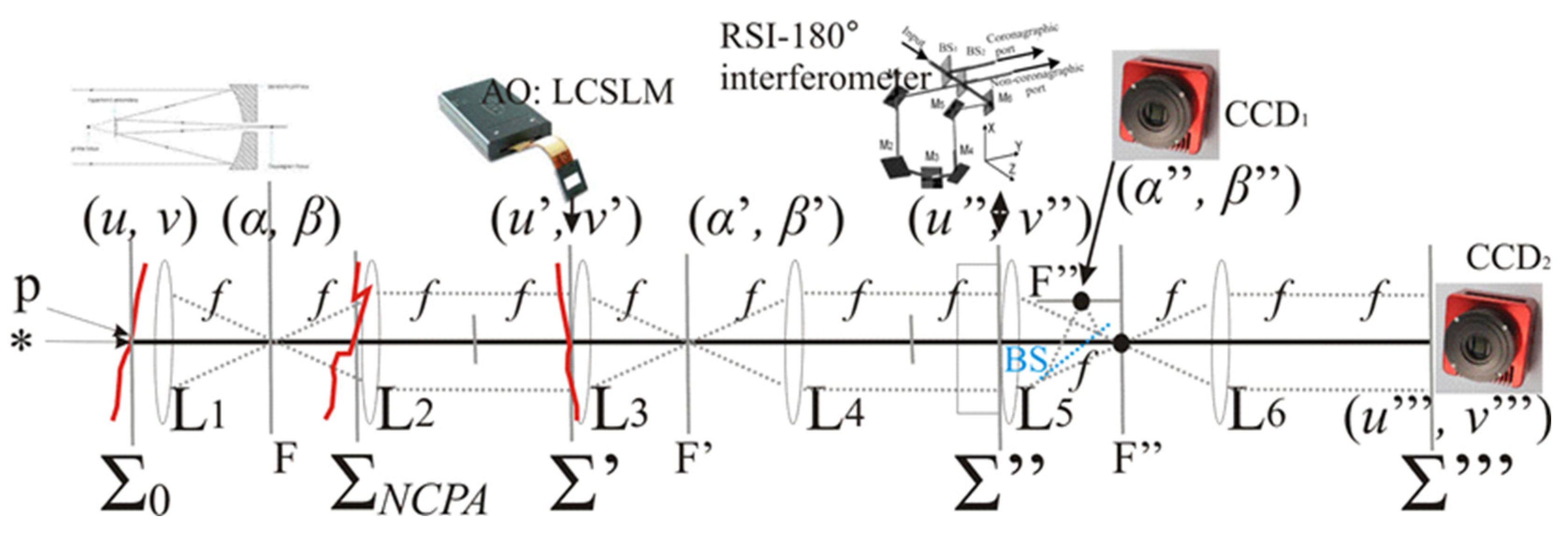
2. Materials and Methods: Common-Path Rotational-Shear Interfero-Coronagraph for Wavefront Measurement

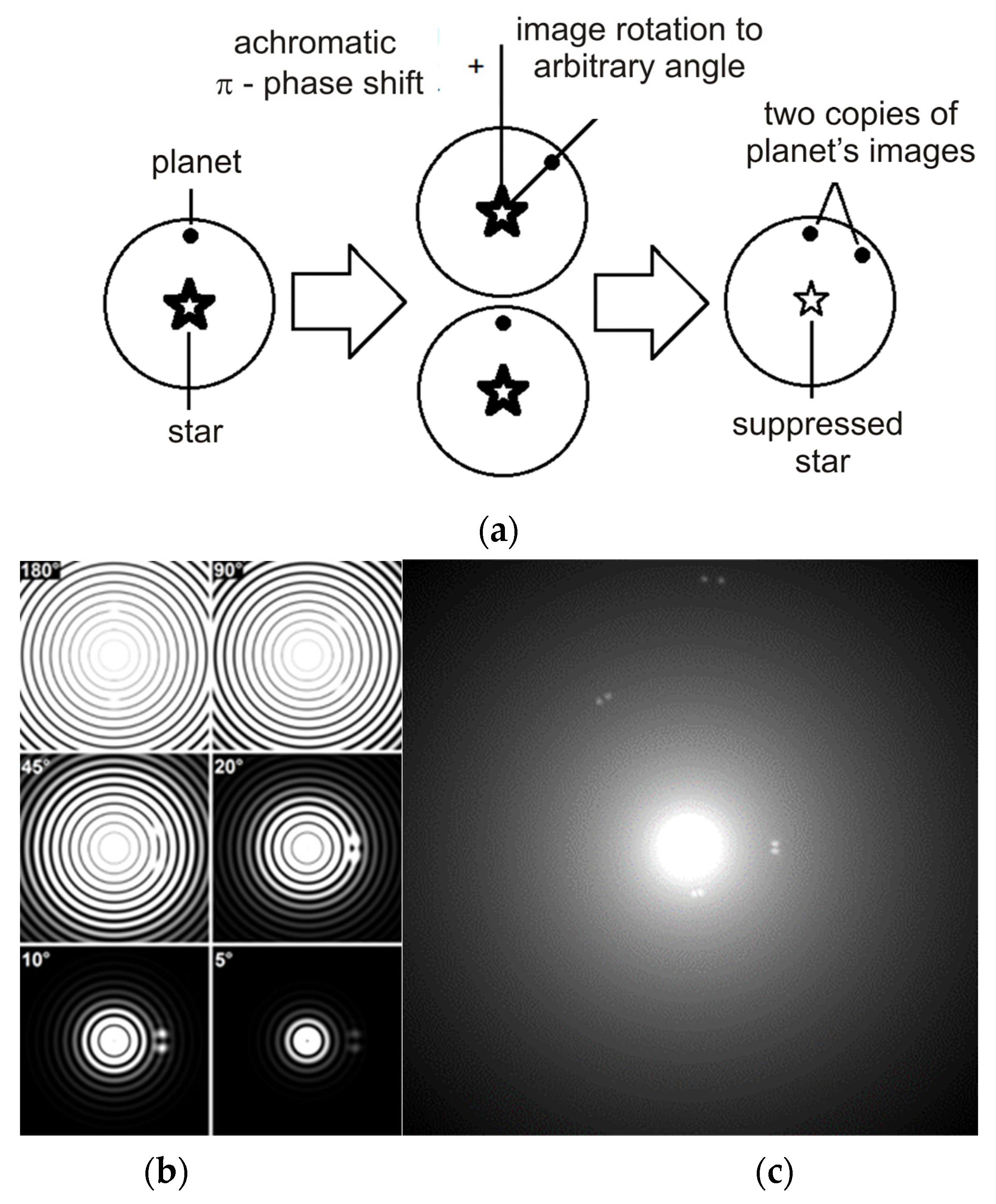
2.1. Common-Path Rotational-Shear Interfero-Coronagraph Principles

In an interfero-coronagraph, the stellar image component is suppressed as the result of destructive interference (with achromatic anti-phase). Stellar light interference occurs after a beam combiner by the on-axis superposition of two copies of a star image being mutually rotated by a certain angle of rotational shift (relative to the optical axis). Considering a point-like star as a light source, after beamsplitter, two point-spread-functions (PSFs) of the star image are set to be geometrically superimposed and, therefore, are suppressed (canceled) by destructive interference at dark port. The main energy of stellar PSF is re-directed to the bright port of interferometer. At the same time, off-axis image components—two PSFs from non-central regions of the image—(we assume an off-axis PSF is an exoplanet)—become geometrically separated (at least partially). Off-axis PSFs are non-superposed due to the rotational shift about the optical axis centered to stellar PSF. An exoplanet PSF cancelation or even its significant attenuation does not occur. This principle is explained in Figure 1a.
With an interfero-coronagraph, starlight suppression cannot be complete due to the physical size of a star. An apparent non-infinitesimal stellar disk size, as observed from a distance of several parsecs, effects an extended light-source. However, rather different suppression amounts of starlight can be achieved [13,14,15] if one varies the rotational shear by the angle; see Figure 1b. Here, the planet components with the peak contrast of ε = 10−8 = (Stellar PSF peak)/(Planet PSF peak) are visually saturated (or overwhelmed) by starlight leaked at the rotational shears of ψ = 180°, 90°, and 45°. A planet at a 5∙λ/D separation with a ε = 10−8 contrast can be clearly visualized at the rotational shear less than ψ = 20°; see corresponding panels. By the smaller angle of rotation shear (e.g., 5°), the planet images also become suppressed.
To illustrate an interfero-coronagraph applicability, in Figure 1c, we represent the simulated picture of the Solar System as observed from 10 pc in polychromatic band (λ = 350–850 nm) with a telescope having an ideal optics D = 2.4 m with an ideal optics interfero-coronagraph attained at ψ = 3.6° angular shear. We visualize Jupiter, Saturn, Uranus, and Neptune (double-dots images) when we trace them toward the periphery.
To verify, one can use Equation (1), which describes the intensity of residual light [15] because of the starlight leakage effect (because of apparent stellar size). Stellar PSF residual is in the first summand, and the intensity of planet light splits in two PSFs—in the second and third summands.
I ( α ,   β ) = Θ 2 4 sin 2 ψ 2 ( J 2 2 ( π D ρ / λ ) ρ 2 ) + ε 1 4 × [ A ( α ρ 0 cos ψ 2 ,   β ρ 0 sin ψ 2 ) A ( α ρ 0 cos ψ 2 ,   β + ρ 0 sin ψ 2 ) ] 2 ,
where
α and β—position angles on the celestial sphere α 2 + β 2 =   ρ 2 :
α = 0 , β = 0 —co-ordinates of a star (on-axis);
ρ 0 ( α 0 ,   β 0   ) —stellar-centric co-ordinates of a planet (off-axis);
Θ —apparent stellar size, e.g., Θ ≈ 0.02   λ / D (@ λ = 500 nm, D = 2.4 m);
ψ —angle of rotational shift;
ε = ( S t e l l a r   P S F   p e a k ) / ( P l a n e t   P S F   p e a k ) —peak-to-peak star-to-planet luminosity ratio;
A ( α ,   β   ) = 2 J 1 ( π D ρ / λ ) / ( π D ρ / λ ) —planet PSF assumed here having the equal luminosity to the stellar PSF;
J 1 ,   J 2 —first and second-order Bessel function of the first kind;
D —telescope diameter;
λ —sensing wavelength.
Without any image post-processing technique, a raw coronagraphic contrast (denoted CC) defines the ratio of planet light amount to residual light at the image area integrated over a spatial domain denoted by S. Area S can be chosen equal to the PSF core and for a central wavelength in Δ λ domain, Equation (2).
C C ( ρ 0 , ψ , Θ   ) = Δ λ S [ p l a n e t   l i g h t   ( λ , D , ρ 0 , ψ , α , β ) ] d λ d α d β Δ λ S [ r e s i d u a l   s t a r   l i g h t   ( λ , D , Θ ,   ψ , α , β ) ] d λ d α d β = Δ λ S 1 4 × [ A ( α ρ 0 cos ψ 2 ,   β ρ 0 sin ψ 2 ) A ( α ρ 0 cos ψ 2 ,   β + ρ 0 sin ψ 2 ) ] 2 d λ d α d β Δ λ S Θ 2 4 sin 2 ψ 2 J 2 2 ( π D ρ / λ ) ρ 2 d λ d α d β .
Published in [15], the table of Equation (2) evaluates the CC contrasts versus the star-to-planet separation ρ 0 , and the rotational shift ψ shows the possibility to visualize giant planets orbiting a Solar-type star from 10 pc with D = 2.4 m telescope at λ   = 500 nm as Jupiter in the Solar System (SS) at ρ 0 ≈ 12.1 λ / D , with ψ ≈ 7.5° with l o g ( C C ) ≈ −8.8. However, telluric planets such as the Earth in the SS can be observed at ρ 0 ≈ 2.3 λ / D separation with ψ ≈ 40° and, by contrast, l o g ( C C ) ≈ −5.0. Image processing can enhance one or two orders in CC contrast. We can optimistically visualize a Jupiter-like SS exoplanet and cannot visualize an Earth-like planet without processing about 5 orders of magnitude in the contrast that remains almost out of detector dynamic range.
Previously, without wavefront correction issue, we have experience with the nulling interferometers having different rotational shears [11,15]. We designed optical assemblies with out-of-plane principal ray propagation via successive reflections on plane mirrors. Several nulling optical schemes with the mutually balanced amplitudes of interfering waves by rotational-shear interferometers (RSI) are represented in Figure 2. The designed common-path nulling interferometers have the various numbers of reflections and the different amounts of rotational shear; moreover, the latter can be fixed or variable. Following the schemes in Figure 2, after the second beam splitter BS2 (a) or after polarizing beam splitter PBS2 in (b,c), we constructed a closed loop for a common optical path via successive mirror reflections. Indeed, two interferometer arms share the same path, are contrary directed, and, therefore, they have no optical path differences. Such a zero-difference in optical path lengths allows the achromatic functioning of the coronagraph. Rotational shear architecture achieves maximum transmission in the absence of pupil shielding. Shown in Figure 2, designs were tested under laboratory conditions, and their functionalities as achromatic coronagraphs were lab demonstrated [11,15].
The interfero-coronagraph in Figure 2a has the 180° scheme, the Figure 2b scheme has a variable rotational shift, and the Figure 2c scheme has a fixed angle of rotation shear. The schemes of Figure 2b,c are characterized by increased sensitivity to polarization inhomogeneities across the aperture due to three successive polarization elements being installed in optical train: two polarization beam splitters and a half-wave plate. The wave plate is designed to be optimized to the central wavelength of a working spectral range, and its purpose is to increase the transmission of the coronagraph. Wave-plate has principal achromaticity, but it is not a critical issue for coronagraphic contrast at non-central wavelengths. To detail more functional and engineering aspects of these interfero-coronagraphs, we refer the reader to our former publications [11,15].
For simplicity, in the present work, we study an interfero-coronagraph with 180° only (shown in Figure 2a), with a function for wavefront sensing. With minor algorithm modifications, other nulling interferometers can perform similar wavefront measurement techniques.

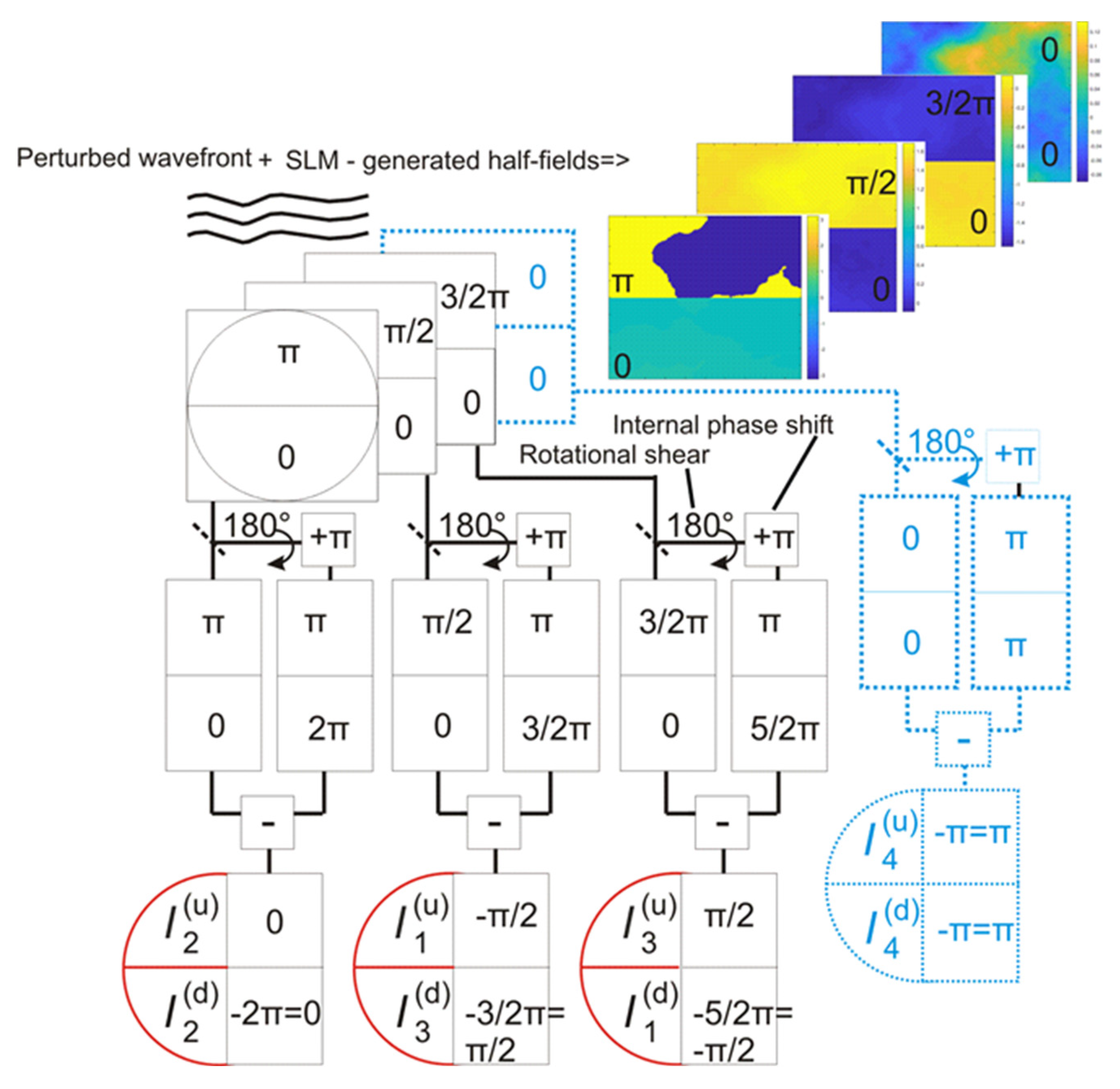
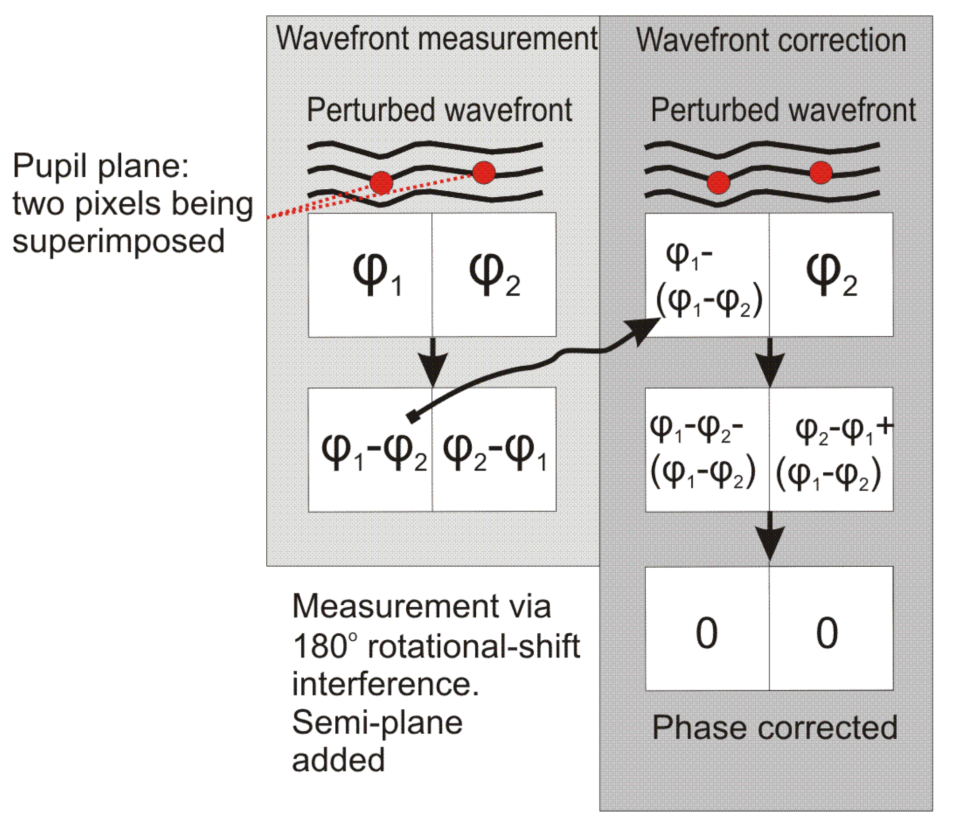
2.2. Wavefront Measurement by Means Interfero-Coronagraph and Phase Shifting Interferometry

By means of an RSI-180° interfero-coronagraph, we implemented a PSI (phase shifting interferometry) technique to measure the interference fringes visibility γ ( u , v ) (from which we can characterize the amplitude distribution P ( u , v ) ) and the ϕ ( u , v ) phase distribution of the electric field in a pupil plane ( u , v ) . Applying the PSI technique to coronagraphy, we found this approach is rather different from, e.g., EFC [17]. To find an incident wavefront characteristic, we solve the inverse problem substantially easier. We found, however, much closer similarity of PSI with [25,26].
In Section 2.1, we have already introduced angular sky coordinates set at (α, β) on a celestial sphere. Setting Cartesian coordinates, denoted as ( x , y ) , in the image plane conjugated to the focal (or CCD) plane can be found by ( x = sin α cos β , y = sin α sin β ) . Complex amplitudes in the pupil ( u , v ) and in the image ( x , y ) are Fourier transformed: P ^ ( x , y ) e i ϕ ^ ( x , y ) = F 1 { P ( u , v ) e i ϕ ( u , v ) } .
To enable a wavefront measurement by PSI, we detect the intensities of several interference patterns obtained by a set of controlled phase shifts in the plane conjugated to the pupil. To measure the wavefront by interfero-coronagraph (with a 180° rotational shift), we perform sequentially the phase-step modulation in the half of pupil field. Before the interferometer, a pixelated AO element (LC SLM) was installed in a conjugated pupil. Then, using the PSI formulas, we recover the wavefront considered as referenced to a half view field via a 180° rotational shear interferometer.
For PSI details, we refer the reader to [23]. Just to briefly recall phase-shifting interferometry (PSI), let us fix the reference mirror position in one arm of the Michelson interferometer; in the second arm of the interferometer, the mirror is cyclically shifted along the optical path by a multiple of the phase shift ϕ i , and the corresponding intensity distributions I i ( u , v ) are measured. Three-, four-, and multi-step PSI techniques are therefore known [23].
The simplest three-step PSI technique assumes a constant phase step modulation with ϕ i : ϕ , 0, and ϕ . When ϕ = π/2, one measures three consecutive intensity values: I ( u , v ) ϕ = π / 2 = I 1 , I ( u , v ) ϕ = 0 = I 2 , and I ( u , v ) ϕ = π / 2 = I 3 , can calculate the phase distribution ϕ ( u , v ) and the module of the coherence function denoted by γ ( u , v ) , which is simplified as the fringe visibility or the mutual amplitude of two interfering waves. The four-step method is more accurate with the same step ϕ = π/2. When four intensity distributions are collected, respectively, the phase shifts: −π/2, 0, π/2, π: I ( u , v ) ϕ = π / 2 = I 1 , I ( u , v ) ϕ = 0 = I 2 , I ( u , v ) ϕ = π / 2 = I 3 , and I ( u , v ) ϕ = π = I 4 . The generalization of three- and four- is a more accurate N-step algorithm. Corresponding formulas to recover the   ϕ ( u , v ) phase and the γ ( u , v )   visibility distributions from the fringe patterns I 1 . . I l by the three-step-, the four-step, and the N-step PSI methods, are shown in Table 1.
The implementation of the three-step PSI in the 180° rotational-shift interferometer is shown in Figure 3; here, the algorithm of the four-step method is complemented by the dashed blue color on the right. For illustration in the upper-right corner, four color panels simulated with Proper [27] show the mixture of semi-plane modulation with background phase perturbation pattern. We use the phase modulation of the half of pupil field and obtain intensities I 1..3 or I 1..4 according to the PSI algorithms.
Therefore, the wavefront with some initial phase distribution ϕ ( u , v ) undergoes an additional phase shift ϕ , uniform in a half of the pupil plane. Wave propagation in the interfero-coronagraph arms follows the mutual image rotation to ±90° and results in a 180° rotational shift. An internal achromatic phase shift of π radian is implemented between the interferometer arms (schematically shown in Figure 3 in one interferometer arm). These processes determine the optical waves superposed by their interference with some fixed set of uniform phase modulations; see Figure 3. The corresponding phase shifts in the half-pupil make interference pattern intensities (as denoted by the superscripts indices (d)—lower half-field and (u)—upper half-field) suitable for PSI. These intensity maps can be easily constructed in a computer memory from field-halves to full fields; they are shown at the bottom of Figure 3 with the indices corresponding to three- and four-step PSI techniques as I 1..3 , 4 ( u ) , I 1..3 , 4 ( d ) . The implementation of the four-step method is shown in blue and dashed on the right. Finally, from intensities I 1..3 , 4 , PSI technique recovers the phase ϕ ( u , v ) distribution and the fringe visibility γ ( u , v ) distribution (following Table 1).
Measured in this way, the phase distribution ϕ ( u , v ) in the pupil semi-plane is sufficient to compensate the observable wavefront aberrations by sending ϕ ( u , v ) or + ϕ ( u , v )   distribution to AO LC SLM, depending on a chosen halfplane on SLM.
Interfero-coronagraph with an implemented 180° rotation-shift automatically suppresses the symmetric image components as originated from the initial even numbers (symmetric) wavefront aberration terms in an incident wave up-streaming to coronagraph. By the PSI modulation described above set by an LC SLM (as the main pixilated AO element), we measure distorted phase distribution ϕ 0 ( u , v ) originally made from the asymmetric image components from the odd number of wavefront aberrations in an incident wave. Noting an off-axis planet PSF is an example of an odd number aberration. After the 180° interfero-coronagraph, odd number aberrations become added, with the aberration located geometrically symmetric respective to optical axis: ϕ Σ ( u , v ) =   ϕ Σ ( u , v ) . By this way, a ghost centro-symmetric copy of planet PSF is always observed. The subscript   Σ stands to define the succeeding pupil plane after (or downstream to) coronagraph, which is optically conjugated to the plane, denoted further as Σ = Σ 0 , where the incident phase distribution ϕ 0 ( u , v ) was considered.
These wavefront measurement and correction techniques by 180° interfero-coronagraph with an AO LC SLM before the 180° interfero-coronagraph are illustrated in Figure 4.
Here, we consider, in initial perturbed wavefront (phase distribution), two (red-marked) pixels which come later in the destructive interference process by their superposition. We denote by φ 1 and φ 2 the corresponding phases in these two pixels. The next row shows conjugated pixels in the plane after superposition the phases φ 1 and φ 2 are subtracted by interference. By PSI, one recovers phase pattern in (e.g., left) semi-plane as simplistic, and one considers phase difference φ 1 φ 2 from the corresponding pixels. For following wavefront correction, one assumes a left semi-plane phase distribution and sends its negative value to AO LC SLM into the corresponding pixel in left semi-plane. To illustrate this correction, in Figure 4, we can see in the right column the left pixel becomes phase modulated, while the right pixel does not have any additional modulation. As the result of the superposition, we see the phase becomes further corrected in both pixels in both semi-planes.

3. Results

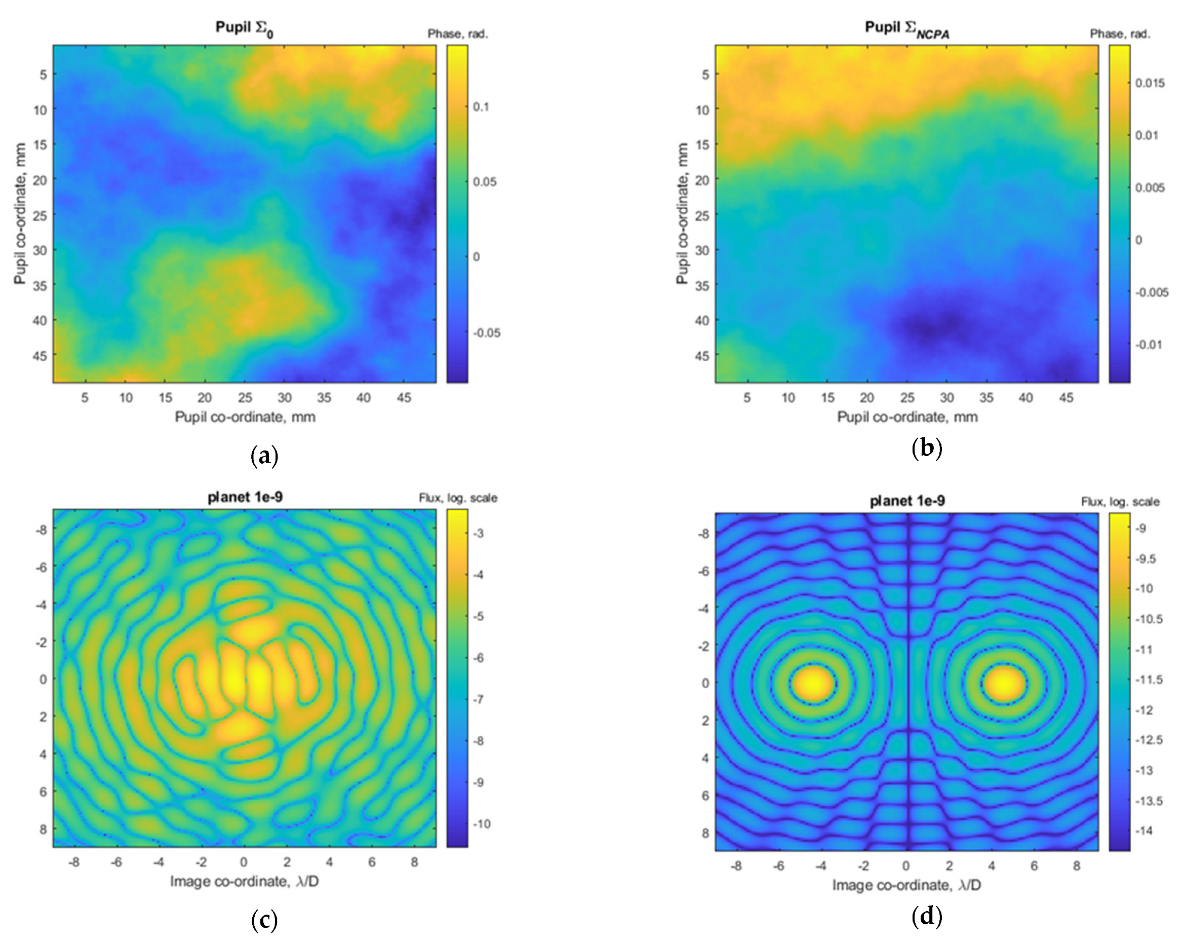
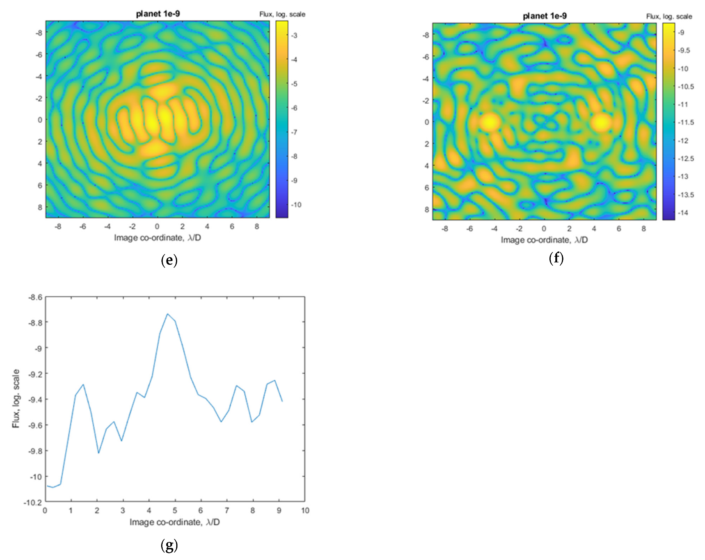
3.1. Numerical Simulation of Wavefront Control in an Optical Scheme with an Interfero-Coronagraph

To verify the applicability of the PSI technique to function in a 180° interfero-coronagraph, we have performed numerical simulations. In the PROPER [27] software package, we added several new blocks (i) to determine the phase and the amplitude distributions in optical pupil by PSI technique and (ii) to simulate a 180° interfero-coronagraph and to visualize its output. We considered the optical scheme shown in Figure 5, containing a telescope (shown by lens L1) and optical elements (lenses L2..6) in order to make several optical planes (with co-ordinates), Σ′ = (u′, v′), Σ″ = (u″, v″), and Σ‴ = (u″, v″) being optically conjugated to the primary pupil Σ0 = (u, v). Aberrations of the telescope are resumed in Σ0. AO element—LC SLM is installed in the secondary pupil Σ′. Interfero-coronagraph is placed in the space before the tertiary pupil Σ″. In the next pupil Σ″″, we place CCD2, which is used to measure wavefront by recording a series of PSI images I 1 . . L . Another CCD1 is the field camera to observe an image in the focal plane F″, which is illuminated (shown in blue) by some beam splitters, assumed to be dichroic or switchable.
We understand that a lot of optical elements and their optical surfaces are placed outside the pupil planes Σ0, Σ′, … Σ‴. Optical surface defects can be optically characterized with power spectral density (PSD) for micro-roughness; these surface figures produce Fresnel-propagation-like aberrations which we can associate with non-common-path aberrations (NCPA). Strictly, the NCPAs have the difference from the aberrations detected by a wavefront sensor (WFS), important in that NCPAs degrade coronagraphic image quality. In our case, because wavefront measurement is organized after the coronagraph, NCPAs (Fresnel aberration screens) generate not only phase errors but also amplitude wavefront errors. In the model, NCPA can be introduced as a phase aberration screen in an intermediate ΣNCPA plane, which is a non-conjugate optically to the pupil. By Fresnel propagation, NCPA results in a high spatial frequency amplitude (and phase) modulation of the pupil. Therefore, NCPAs’ effect can be studied if one considers several aberration screens in mutually non-conjugated planes (ΣNCPA1, ...). In Figure 5, we show a single ΣNCPA plane.
To simplify the evaluation of aberrations’ influence on a coronagraphic image and to study residuals after wavefront correction, Figure 5 shows a generalized optical system with unity magnification and with the equal focal lengths f of the optical lenses, while in a practical design, the magnifications and scales of the images will differ from the simulated parameters.
Figure 6 shows several results from the evaluation of the optical system (Figure 5). Examples of mutually non-correlated aberration phase screens in planes Σ0 and ΣNCPA are shown in Figure 6a and Figure 6b, respectively. These aberrations do not include any classic geometric aberrations (coma, spherical, astigmatic, etc.) as represented by low-order Zernike polynomial decomposition. The shown aberrations consist only of micro-roughness errors, and they visually look like sky clouds. PSD was characterized by the local phase error δ ϕ ~ ρ 2 , where ρ = u 2 + v 2 is the radial scale. The RMS error σ = 10 nm of the wavefront ϕ Σ 0 ( u , v ) in Σ0, and the RMS σ = 1 nm error of the ϕ Σ NCPA ( u , v ) wavefront in ΣNCPA were calculated at the characteristic length of ρ = D / 2 .
In Figure 6c–f, simulated coronagraphic images I(x″, y″) are shown, as observed in the focal plane F″ by a CCD1 field camera. A companion (planet) was computed with the PSFs peak-to-peak contrast C = 10−9 between the point-like light sources planet and star. Contrast C was modeled as C = I * , @ λ I p , @ λ and the wavelength λ = 500 nm. The star (*) and planet (p) were separated at a 5 λ/D stellocentric distance. Panels (c), (d) were calculated with the wavefront distortions ϕ Σ 0 ( u , v ) by σ = 10 nm. In panel (c), the coronagraphic image I(x″, y″) was computed without any wavefront correction. The image contains strong speckle effects, which completely masks the faint planet image. In panel (d), the coronagraphic image was computed as phase corrected, and we applied the phase screen of ϕ Σ 0 ( u , v ) by AO LC SLM in the plane Σ′(u′, v′). Now, both the planet PSF and its ghost symmetric copy were completely cleared of speckles. This is because the optically conjugated planes Σ0 and Σ′ are considered to contain the equal phase distributions, which were compensated for. In panels (e) and (f), besides the initial aberration ϕ Σ 0 ( u , v ) , an additional ϕ Σ NCPA ( u , v ) aberration in different and not conjugated plane ΣNCPA was computed. In panel (e), correction was not applied, and this image is nearly similar to that in panel (c). In panel (f), correction was applied by setting the phase screen ϕ Σ ( u , v ) in the plane Σ′(u′, v′); note that ϕ Σ ( u , v ) ϕ Σ 0 ( u , v ) , which is non-equal to the correction used for result in (d) panel. Moreover, the amplitude distribution P Σ ( u , v ) (not shown) becomes non-uniform across the pupil.
The panel (f) image as compared with the panel (d) image has residual speckles which are caused by non-corrected amplitude distortions in pupil Σ′, as induced by phase aberration ϕ Σ NCPA ( u , v ) in ΣNCPA. Shown in panel (g), the radially averaged profile of coronagraphic image (f) robustly visualizes a companion in 5 λ/D by the intensity maximum.
Shown in Figure 6, the simulation results were obtained by the known phase distributions ϕ Σ ( u , v ) , ϕ Σ ( u , v ) in the plane of wavefront correction of Σ′ = (u′, v′). This is possible in the simulation; however, practically, one needs to measure phase distributions for its corrections. Therefore, next, we have modified our numerical experiment to check how to determine phase ϕ Σ 0 ( u , v ) by the PSI four-step phase-shifting technique downstream from the coronagraph. PSI was applied to half of the pupil plane Σ′(u′, v′) for the wavefront correction in the AO LC SLM plane Σ′(u′, v′). The images obtained by the simulation of the PSI technique have been found to coincide with coronagraphic images shown in Figure 6 in panels (c)–(f).

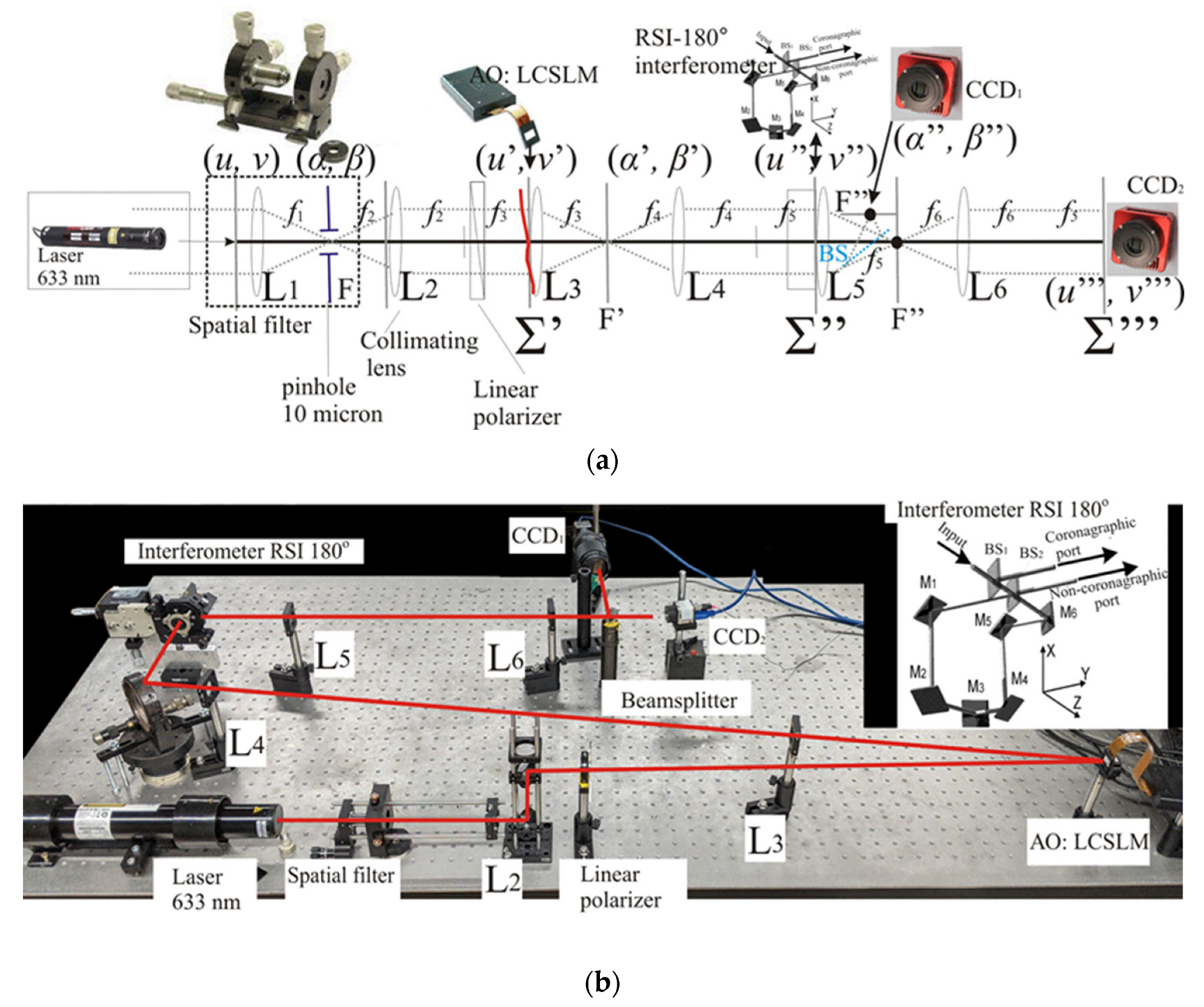
3.2. Lab Experiment to Verify Wavefront Correction

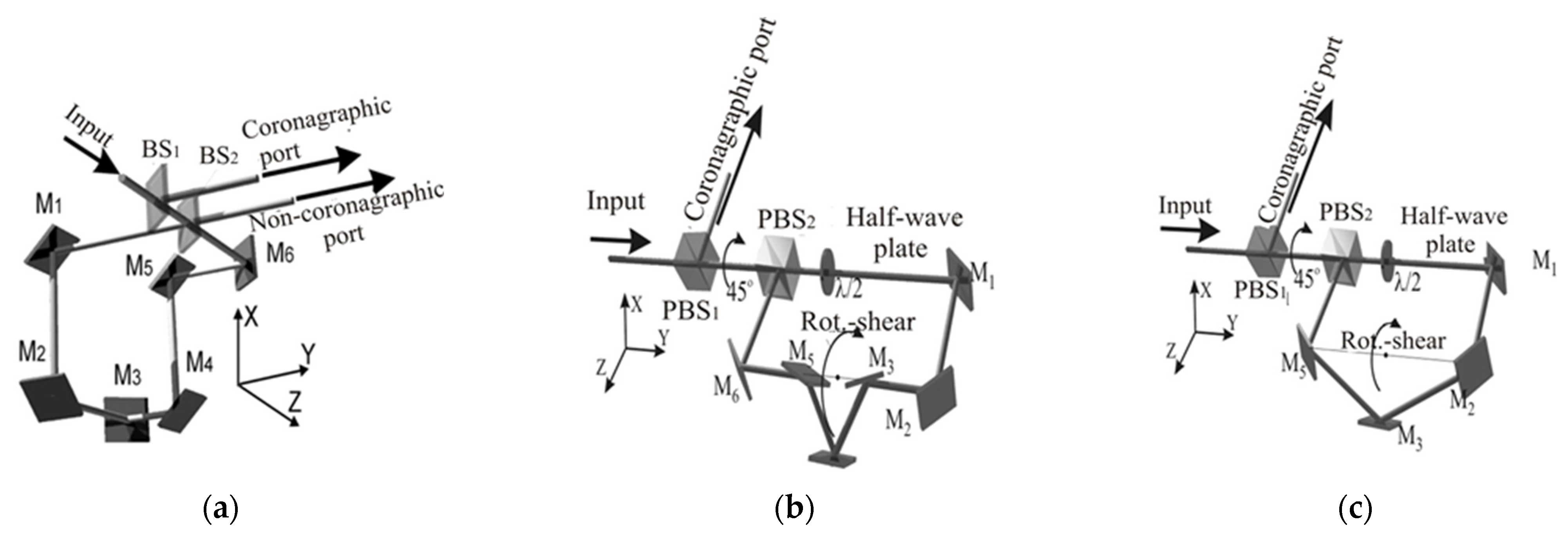
3.2.1. Schematics of Lab Experiment

Schematic and photo of the lab experiment, shown in Figure 7a,b, respectively.
In the lab experiment, light radiation from an HeNe laser passes through a spatial filter, a collimation lens L2, a linear polarizer, and through a reflecting phase-only LC SLM propagating in the direction of the AIC-180°interfero-coronagraph. Lenses L3L4 conjugate optically the pupil plane Σ′ where the LC SLM is installed to the beam combiner plane of the AIC-180° interfero-coronagraph, where interfering waves are superposed. After the coronagraph, another beam splitter BS is located. In this direction after the beam splitter reflects, an image (focal) plane is formed and is observed by a CCD1 field camera. CCD1 stands to observe a coronagraphic image in the focal plane. In the other direction, the beam splitter transmits an image, and an additional lens L6 stands to form an optical pupil plane image. This pupil image is observed by the second CCD2 to measure the wavefront distribution according to the PSI algorithms; see Table 1.

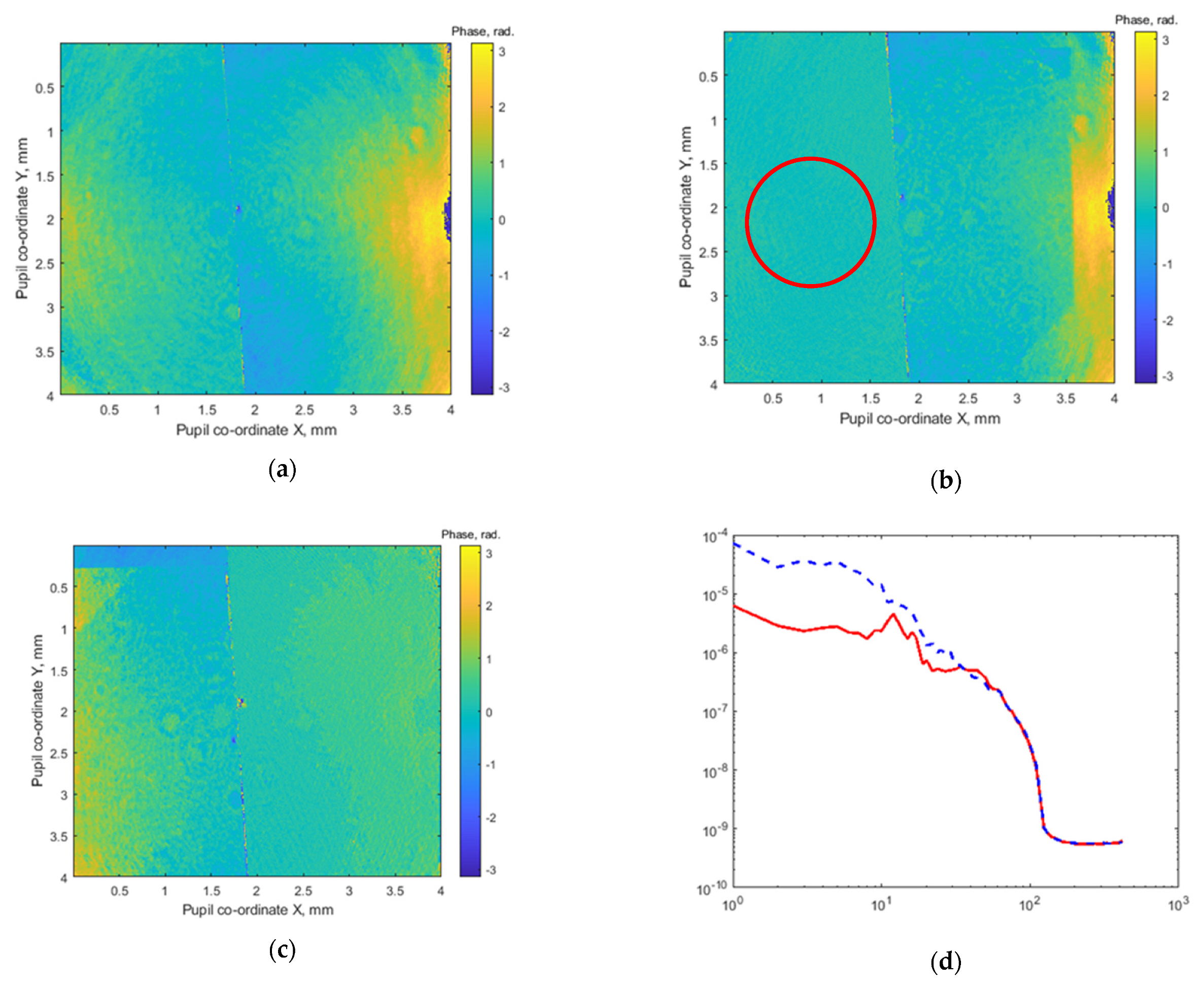
3.2.2. Wavefront Correction Maps in Pupil Plane

Some results of wavefront phase correction based on measurements in the pupil plane via CCD2 applying PSI algorithms (modified as shown in Figure 3) are shown in Figure 8.
Figure 8 shows the correction of a nearly flat wavefront with the initial standard deviation σ ≈ λ/5. The uncorrected wavefront is shown in (a) panel; then, the left and right parts were corrected alternately, as shown, respectively, in panels (b) and (c).
In the optical scheme, the spatial phase modulator LC SLM was installed before the interfero-coronagraph 180°; this schematic has allowed us to only symmetrically influence wavefront distortions simultaneously in two halves of the pupil plane. Because of this schematic feature, all asymmetric wavefront distortions are corrected alternately either in the left or the right halves of the pupil plane.
In Figure 8d, analyzing the radially averaged power spectrum density (PSD) of the pupil half-plane before correction (shown by the blue dashed line) and after (shown by the red solid line), one can see that heterogeneities with spatial frequencies (with characteristic size) less than 1/10 of the half-aperture can be effectively corrected (by more than an order of magnitude), while the higher spatial frequencies are not corrected. Mid- and high-frequency non-correction are explained by the presence of non-common path aberrations, which cause uncontrolled and, therefore, uncorrected amplitude errors in the mid and high frequencies.
Used here is the adaptive optical element; the LC SLM was implemented in phase-only mode. However, it has a potential to correct both the amplitude- and phase wavefront distortions if the LC SLM is rotated respective to the polarization axis.
For this option, the PSI method shown in step-shift mode on the pupil semi-plane (for the 180° rotation shift plane interferometer) is well-suited to measure both the phase and amplitude wavefront distortions for wavefront control by LC SLM, assuming wavefront distortions originated in non-conjugated planes induce high frequency phase–amplitude aberration known as (non-common-path) aberrations (ΣNCPA).

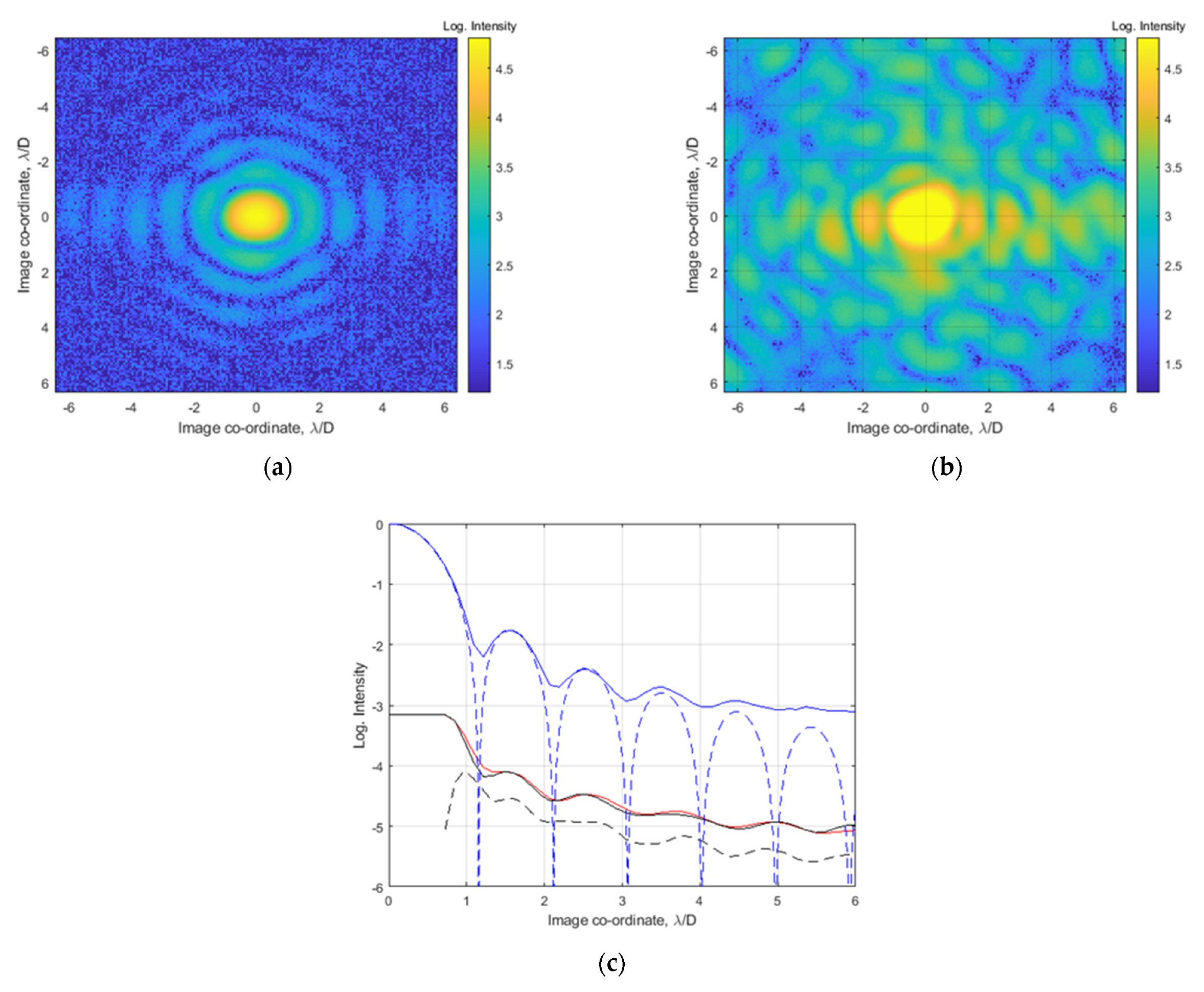
3.2.3. Coronagraphic PSF Suppression in Focal Plane

Phase correction experiments (similar to those in the pupil plane shown in Section 3.2.2) were also observed in the focal (image) plane by CCD1, where coronographic images were recorded. The non-coronagraphic and coronagraphic images shown in Figure 9a,b correspondingly were compared to measure a coronagraphic contrast. To obtain a non-coronographic image (after the coronagraph), the input wavefront contains a step-form phase modulation, and the phase gap between the left and right half-planes was about π (see Figure 4: φ 1 φ 2 = π ). By this method, the non-coronagraphic image looks similar to a theoretical PSF as the diffraction image of a point-like source with clearly observed airy rings. The non-coronagraphic frame was captured with 0.02 ms exposure.
The coronagraphic image in Figure 9b was obtained as a result of the applied wavefront correction algorithm. To register it, an exposure time of 30 ms (versus 0.02 ms for Figure 9a) was used to clearly visualize the speckle field pattern. Next, we resume the radially averaged intensity profiles (Figure 9a,b), taking into account their different exposures to plot them in Figure 9c (blue (solid) and red (solid) lines corresponding to the non-coronagraphic PSF and coronagraphic PSF). The PSF profiles were normalized to the value of the maximum intensity of the non-coronographic image (the blue curve value at stellocentric equals unity). The same figure shows the scaled radially averaged intensity profiles of the coronographic images captured in two consequent frames (black and red curves in Figure 9c). In the region of the central maximum of the PSF (in region of 0 along the stellocentric horizontal axis) of the coronographic images, a “flat top” is observed. This is due to the saturation effect of the CCD1 matrix (see CCD1 in the optical scheme in Figure 7) by 30 ms exposure of the coronographic image. Therefore, the represented non-coronagraphic(Figure 9a) and coronagraphic images (Figure 9b) are shown with their scale respective of their exposure ratio 30/0.02 = 1500.
Figure 9b corresponds to Figure 8b, which is taken simultaneously but in the pupil plane. In Figure 8b, the red circle defines the approximate area of the pupil; this was taken by an additional diaphragm (which is not shown in Figure 7a), the diaphragm was used for the images in Figure 9a,b. The phase map in pupil was measured having the standard deviation of σ ≈ λ/40 over the corrected pupil area, marked with a red circle.
Figure 9c enabled the estimation of the coronagraphic contrast (as the ratio of the non-coronagraphic PSF maximum to the scattered light coronagraphic intensity at a given stellocentric distance), which gives ~ 10 5 at >4 λ/D.
In Figure 9c are plotted: the radial cross-section of the theoretical PSF ( 2 J 1 ( r ) / r ) 2 —he blue dashed line, the averaged radial cross-section of non-coronagraphic PSF (a)—blue solid line, two averaged radial cross-sections of coronagraphic realizations at different times—solid black and red lines (b), the black dashed line made by the difference between the two coronagraphic images obtained at different time. The difference in coronagraphic images implies post-processing, in which so-called static speckles are allowed to subtract and show the possibility of an additional gain in coronagraphic contrast. Assuming possible post-processing, in the stellocentric region, wider than the second airy ring (>2 λ/D), we experimentally obtained a coronagraphic contrast of 105 above the PSF value at the maximum, (see black dashed line). Post-processing can improve this value by an order of magnitude, which has not yet been shown in the presented laboratory experiment and will require a greater number of processed images.

3.3. Constraints and Their Overcome

3.3.1. Using an LC SLM for Extreme Wavefront Correction

In the laboratory experiment, we used an LC SLM commercially available (in the Russian Federation) instead of a precision deformable mirror (DM). The LC SLM choice has some advantages and some disadvantages, which are worth noting in the context of the liquid crystal spatial light modulator-based adaptive optics to function for the stellar coronagraph.
Among the advantages of the LC SLM [28] is (i) the significantly higher number of addressable pixels over 1500 × 1000 = 1.5 × 10⁶ compared to the lower number of DM actuators ~103...104. (ii) An amplitude-phase modulation and a general polarization modulation are both possible when using polarization devices. Amplitude-phase modulation occurs, e.g., when two linear polarizers are placed, one before and one after the LC SLM, and polarizers are oriented at their transmission axis at different angles from the direction of the main working polarization axis of the LC SLM. (iii) It is possible to realize an arbitrary wavefront surface, including wavefront discontinuities, which is practically impossible with the DM.
The main drawback of AO LC SLM is the significantly lower accuracy of phase modulation, nominally λ/250 ≈ 2π/28 (i.e., λ/256), at which the corrected wavefront does not have a sufficient quality for observing exoplanets. However, AO LC SLM phase modulation accuracy can be enhanced if an initial phase distortion is within, e.g., λ/10 P-V and has to be corrected. Such a calibrated AO LC SLM performs λ/2500 ≈ 0.1 π/28 radian accuracy.
There are also pixel boundary effects different from the DM due to the physical boundaries of the pixels; here, the relative sizes of the modulated and non-modulated zones are described by the fill factor. Different to LC SLM, a DM has no visible boundaries (on the side of the deformable mirror) between the actuators, but the customized function (named as formfactor) is used to accurately approximate the phase distribution over a discrete number of actuators, taking into account the features of the interconnection between the actuators in deformable mirror to crosstalk the neighboring actuators. Finally, the LC SLM chromaticity, due to the dispersion properties of the liquid crystal material, should be taken into account compared to the DM with the effective free-space dispersion d to modify an optical path length 1 λ .
Let us discuss the main drawback in the insufficient accuracy of the liquid crystal spatial modulator and sketch possible ways to function the LC SLM as an adaptive optics to correct the wavefront for stellar coronagraph. A way to effectively increase the phase modulation accuracy (by more than an order of magnitude) is possible if one applies the principle of an (extremely) unbalanced interferometer [29]. Thus, in a two-beam unbalanced interferometer, two coherent waves are superposed with unequal amplitudes; for example, differing by an order of magnitude (or, in the general case, by a factor of k). Inside the unbalanced interferometer in one arm, the phase of the wave having a smaller amplitude is corrected within the limited accuracy of LC SLM in phase modulation. In the other arm of the interferometer, the phase of the more intensive wave remains unmodulated by an LC SLM. These two waves interfere after a beam combiner.
If one measures the depth of the phase modulation of the resulting wave after the interference process, phase modulation depth will be less than the depth of the phase modulation of the weak amplitude wave. This principle can effectively reduce the modulation error. A detailed description of this method can be found in [29], noting that under the atmosphere, the wavefront is distorted by turbulence and contains a significant wavefront error exceeding several wavelengths in optical range at ~1000 nm. Unbalanced in amplitude, the interferometer can increase the accuracy of the wavefront correction if the wavefront error is substantially smaller than the wavelength λ (at least by an order of ~λ/10...~λ/100). It is, therefore, possible to use two-pixel actuators with accuracy on the order of λ/100, one mounted at the input before the unbalanced interferometer and the other inside the interferometer in the smaller amplitude arm, for accurate wavefront correction in ground-based telescope mode. In an orbital space telescope, a diffraction-limited image is obtained so that the distortion of the wavefront is usually several times smaller than the central wavelength λ. The LC SLM can also be used here in an unbalanced interferometer in a quasi-static mode.

3.3.2. Using an LC SLM for Wavefront Correction in Phase–Amplitude Mode

For the phase modulation mode, the linear polarization at the input has to be set parallel to the working (active) axis of the LC SLM. Here, the corresponding Jones vectors are:
[ E x E y ] = [ e i φ 0 0 1 ] [ 1 0 ] = e i φ [ 1 0 ] .  
Suppose the AO LC SLM is set by its main working axis rotated in respect to the polarization axis of the incoming wave by a non-zero angle. Instead of phase modulation, a modulation of polarization in general form is carried out.
To organize a phase–amplitude modulation mode, we consider a linear polarization at the input that is set at a certain angle—for example, 45 degrees—to the direction of the working (active) axis of the LC SLM. Additionally, to prevent a polarization modulation, we consider using a polarizer (parallel to the initial linear polarization):
[ E x E y ] = R 45 [ 1 0 0 0 ] R 45 [ e i φ 0 0 1 ] 1 2 [ 1 1 ] = 1 2 2 ( e i φ + 1 ) [ 1 1 ] ,
where R β = [ cos β sin β sin β cos β ] is the rotation matrix by angle β.
Further, we consider the fact that the interfero-coronagraph is a shear interferometer. Physically, it causes the coherent superposition (summation) of two waves. Two different pixels of LC SLM—let us denote them as “1” and “2”—become superimposed by an anti-phase to process the destructive interference. For a rotational-shear interferometer RSI-180° (see Figure 2), “1” and “2” are centro-symmetric relative to the rotation axis. When considering the modulation given by (4) set in two pixels “1” and “2” with independently controlled phases φ1 and φ2, it becomes possible to compensate for the initial phase and amplitude modulation in these pixels A 01 e i φ 01 ,   A 02 e i φ 02 . By φ1 and φ2 control, we can equalize the optical fields in pixels in the form of the equal complex amplitudes and phases. When solving the following equation:
A 01 e i φ 01 ( e i φ 1 + 1 ) = A 02 e i φ 02 ( e i φ 2 + 1 )
we search the roots of φ1 and φ2, reducing the number of variables from four to two: φ = φ 01 φ 02 means the difference of initial phases and a = A 01 / A 02 means the ratio of amplitudes:
a e i φ ( e i φ 1 + 1 ) = ( e i φ 2 + 1 ) .
We checked the solution existence for (6). The study of its practical applicability is scheduled for a future work. We hope to use this approach to organize phase–amplitude wavefront corrections aiming to work out a non-common path aberration effect, an amplitude imbalance from some kind of Fresnel type wavefront distortion that originated in the non-conjugated plane to the pupil.

4. Discussion

We have investigated, both in a theoretical model and in a laboratory experiment, a new technique to correct the wavefront required to observe exoplanets in an astronomical diffraction-limited image in the vicinity of a star at stellocentric distance of about several diffraction radii from the parent star. The proposed methodology is workable in terms of measuring and correcting the wave front. In particular, the imaging of the Earth in the vicinity of the Sun, with contrast 109, requires a correction accuracy better than λ/500 on controllable 500 × 500 pixels.
This is achieved by a combination of extremely precise active adaptive optics (ExAO) systems and the coronagraph. In the process of correcting the wavefront, a nontrivial task is solved to measure the wavefront after the coronagraph, where aberrations of the non-common path are taken into account. Therefore, widely used wavefront sensors (e.g., Shack–Hartmann principle based sensors) appear inaccurate and contain additional sources of errors.
The new, currently proposed method for measuring and correcting the wavefront demonstrates in a simple experiment the wavefront quality is better than λ/40, which is still about an order of magnitude worse than the required value (λ/500–λ/1000). An achievement of the target accuracy in wavefront correction will be improved in future work with the possible involvement of additional techniques. With the correction accuracy achieved, the experimental coronagraphic contrast is shown to be better than 105 at a stellocentric distance of more than 2 diffraction radii (~2 λ/D) at a wavelength of 633 nm.
To sum up, the obtained results agree with the theoretical estimates. For the standard deviation σ of the phase of wavefront, a primitive estimation of starlight suppression via the destructive interference process is:
I 0 I = 1 c o s ( σ ) σ 2 2 .
which, for σ = 2π/40, gives 10 2 . Therefore, for a coronagraphic PSF at a distance of 5 λ/D, (7) shows the coronagraphic contrast estimate of 10 5 , which was experimentally demonstrated.

Author Contributions

Conceptualization, methodology, A.T. and A.Y.; software, I.S.; experiment, A.T., A.Y., A.K. and A.L.; writing—original draft preparation, A.Y.; supervision, A.T. and O.K. All authors have read and agreed to the published version of the manuscript.

Funding

This research received no external funding.

Institutional Review Board Statement

Not applicable.

Informed Consent Statement

Not applicable.

Data Availability Statement

The data presented in this study are available on request from the corresponding author.

Acknowledgments

The authors are grateful to the Government of the Russian Federation and the Ministry of Higher Education and Science of the Russian Federation for support under Grant No. 075-15-2020-780 (N13.1902.21.0039).

Conflicts of Interest

The authors declare no conflict of interest.

References

  1. Traub, W.; Oppenheimer, B. Direct imaging of exoplanets. In Exoplanets; Seager, S., Ed.; University of Arizona Press: Tucson, AZ, USA, 2011; pp. 111–156. Available online: https://www.amnh.org/content/download/53052/796511/file/DirectImagingChapter.pdf (accessed on 19 January 2023).
  2. Guyon, O. Extreme Adaptive Optics. Annu. Rev. Astron. Astrophys. 2018, 56, 315–355. [Google Scholar] [CrossRef]
  3. Proposed Missions—Terrestrial Planet Finder. Available online: https://www2.jpl.nasa.gov/missions/proposed/tpf.html (accessed on 19 January 2023).
  4. Lindler, D.J. TPF-O design reference mission. In UV/Optical/IR Space Telescopes: Innovative Technologies and Concepts III; SPIE: Bellingham, WA, USA, 2007; Volume 6687, pp. 406–414. [Google Scholar] [CrossRef]
  5. Large Binocular Telescope Interferometer. Available online: https://nexsci.caltech.edu/missions/LBTI/ (accessed on 19 January 2023).
  6. Noecker, M.C.; Zhao, F.; Demers, R.; Trauger, J.; Guyon, O.; Kasdin, N.J. Coronagraph instrument for WFIRST-AFTA. J. Astron. Telesc. Instrum. Syst. 2016, 2, 011001. [Google Scholar] [CrossRef]
  7. The Nancy Grace Roman Space Telescope. Available online: https://www.jpl.nasa.gov/missions/the-nancy-grace-roman-space-telescope (accessed on 19 January 2023).
  8. Guyon, O.; Pluzhnik, E.A.; Kuchner, M.J.; Collins, B.; Ridgway, S.T. Theoretical Limits on Extrasolar Terrestrial Planet Detection with Coronagraphs. Astrophys. J. Suppl. Ser. 2006, 167, 81–99. [Google Scholar] [CrossRef] [Green Version]
  9. Baudoz, P.; Rabbia, Y.; Gay, J. Achromatic interfero coronagraphy. Astron. Astrophys. Suppl. Ser. 2000, 141, 319–329. [Google Scholar] [CrossRef]
  10. Tavrov, A.V.; Kobayashi, Y.; Tanaka, Y.; Shioda, T.; Otani, Y.; Kurokawa, T.; Takeda, M. Common-path achromatic interferometer–coronagraph: Nulling of polychromatic light. Opt. Lett. 2005, 30, 2224–2226. [Google Scholar] [CrossRef] [PubMed]
  11. Aimé, C.; Ricort, G.; Carlotti, A.; Rabbia, Y.; Gay, J. ARC: An Achromatic Rotation-shearing Coronagraph. Astron. Astrophys. 2010, 517, A55. [Google Scholar] [CrossRef]
  12. Tavrov, A.; Korablev, O.; Ksanfomaliti, L.; Rodin, A.; Frolov, P.; Nishikwa, J.; Tamura, M.; Kurokawa, T.; Takeda, M. Common-path achromatic rotational-shearing coronagraph. Opt. Lett. 2011, 36, 1972–1974. [Google Scholar] [CrossRef] [PubMed]
  13. Frolov, P.; Shashkova, I.; Bezymyannikova, Y.; Kiselev, A.; Tavrov, A. Achromatic interfero-coronagraph with variable rotational shear: Reducing of star leakage effect, white light nulling with lab prototype. J. Astron. Telesc. Instrum. Syst. 2015, 2, 011002. [Google Scholar] [CrossRef]
  14. Pueyo, L.; Kay, J.; Kasdin, N.J.; Groff, T.; McElwain, M.; Give’On, A.; Belikov, R. Optimal dark hole generation via two deformable mirrors with stroke minimization. Appl. Opt. 2009, 48, 6296–6312. [Google Scholar] [CrossRef] [PubMed] [Green Version]
  15. Give’On, A. A unified formailism for high contrast imaging correction algorithms. In Techniques and Instrumentation for Detection of Exoplanets IV; SPIE: Bellingham, WA, USA, 2009; Volume 7440, pp. 112–117. [Google Scholar] [CrossRef]
  16. Riggs, A.E.; Ruane, G.; Coker, C.T.; Shaklan, S.B.; Kern, B.D.; Sidick, E. Fast linearized coronagraph optimizer (FALCO) I: A software toolbox for rapid coronagraphic design and wavefront correction. In Space Telescopes and Instrumentation 2018: Optical, Infrared, and Millimeter Wave; SPIE: Bellingham, WA, USA, 2018; Volume 10698, pp. 878–888. [Google Scholar] [CrossRef] [Green Version]
  17. Griewank, A.; Walther, A. Evaluating Derivatives: Principles and Techniques of Algorithmic Differentiation, 2nd ed.; Society for Industrial and Applied Mathematics: Philadelphia, PA, USA, 2008; ISBN 978-0-89871-659-7. Available online: https://epubs.siam.org/doi/pdf/10.1137/1.9780898717761.fm (accessed on 19 January 2023).
  18. Paul, B.; Mugnier, L.; Sauvage, J.-F.; Ferrari, M.; Dohlen, K. High-order myopic coronagraphic phase diversity (COFFEE) for wave-front control in high-contrast imaging systems. Opt. Express 2013, 21, 31751–31768. [Google Scholar] [CrossRef] [PubMed] [Green Version]
  19. Riggs, A.J.E.; Kasdin, N.; Groff, T.D. Recursive starlight and bias estimation for high-contrast imaging with an extended Kalman filter. J. Astron. Telesc. Instrum. Syst. 2016, 2, 011017. [Google Scholar] [CrossRef] [Green Version]
  20. Baudoz, P.; Boccaletti, A.; Baudrand, J.; Rouan, D. The Self-Coherent Camera: A new tool for planet detection. Proc. Int. Astron. Union 2005, 1, 553–558. [Google Scholar] [CrossRef] [Green Version]
  21. Groff, T.D.; Riggs, A.J.E.; Kern, B.; Kasdin, N.J. Methods and limitations of focal plane sensing, estimation, and control in high-contrast imaging. J. Astron. Telesc. Instrum. Syst. 2015, 2, 011009. [Google Scholar] [CrossRef] [Green Version]
  22. Nishikawa, J.; Murakami, N. Unbalanced nulling interferometer and precise wavefront control. Opt. Rev. 2013, 20, 453–462. [Google Scholar] [CrossRef]
  23. Malacara, D. Optical Shop Testing, 3rd ed.; John Wiley & Sons, Inc.: Hoboken, NJ, USA, 2006; ISBN 9780471484042. [Google Scholar] [CrossRef]
  24. Huang, Y.; Liao, E.; Chen, R.; Wu, S.-T. Liquid-Crystal-on-Silicon for Augmented Reality Displays. Appl. Sci. 2018, 8, 2366. [Google Scholar] [CrossRef] [Green Version]
  25. Hénault, F.B.; Carlotti, A.; Verinaud, C. Phase-shifting coronagraph. In Techniques and Instrumentation for Detection of Exoplanets VIII; SPIE: Bellingham, WA, USA, 2017; Volume 10400, pp. 418–439. [Google Scholar] [CrossRef] [Green Version]
  26. Hénault, F. Phase-shifting technique for improving the imaging capacity of sparse-aperture optical interferometers. Appl. Opt. 2011, 50, 4207–4220. [Google Scholar] [CrossRef] [PubMed] [Green Version]
  27. PROPER Optical Propagation Library. Available online: https://proper-library.sourceforge.net (accessed on 19 January 2023).
  28. HOLOYEY Spatial Light Modulators. Available online: https://holoeye.com/spatial-light-modulators (accessed on 19 January 2023).
  29. Shashkova, I.; Shkursky, B.; Frolov, P.; Bezymyannikova, Y.; Kiselev, A.; Nishikawa, J.; Tavrov, A.V. Extremely unbalanced interferometer for precise wavefront control in stellar coronagraphy. J. Astron. Telesc. Instrum. Syst. 2015, 2, 011011. [Google Scholar] [CrossRef]
Figure 1. Rotation-shear interfero-coronagraph: principles and simulated output. (a)—anti-phase superposition on-axis for stellar PSF (asterisk denoted) and doubling off-axis planet’s PSF (dot denoted). (b)—monochromatic starlight incomplete suppression, leakage considering the stellar size of Θ = 0.01 λ/D (@ D = 2.4 m, λ = 500 nm) by various rotational shears (the angles of rotation are noted), the shown planet PSF considered at the stellocentric separation of ρ0 = 5 λ/D, and contrast ε = 10−8. (c)—in polychromatic band (λ = 350–850 nm), picture of Solar System as observed from 10 pc with the telescope D = 2.4 m and the interfero-coronagraph having 3.6° angular shear; Jupiter, Saturn, Uranus, Neptune seen visualized toward periphery.
Photonics 10 00320 g001
Figure 2. Optical schematics of common-path nulling interferometers with various rotational-shear angles acting as interfero-coronagraphs (on their dark port): (a) CP-AIC (RSI-180°) with rotational-shear angle fixed at 180°; (b) RSI-VAR with a variable rotational-shear angle; (c) RSI-10° rotational-shear angle fixed at 10°.
Photonics 10 00320 g002
Figure 3. Phase modulation provided in the pupil semi-plane. Denoted are intensity values I 1..3 ( u ) , I 1..3 ( d ) used by the three-step PSI; the subscripts (u) and (d) stand for the upper and lower halves of the pupil; an additional phase modulation with the corresponding intensities of I 4 ( u ) , I 4 ( d ) for the four-step PSI algorithm is in blue.
Photonics 10 00320 g003
Figure 4. Illustration (in left column) for the measurement of wavefront by 180° interfero-coronagraph and (in right column) for the correction of wavefront by an AO LC SLM placed before the 180° interfero-coronagraph. (Note that here the corrected “left” side of SLM is shown. The same result could be achieved with “right” side just by altering the sign before φ 1 φ 2 ).
Photonics 10 00320 g004
Figure 5. Optical scheme to assemble telescope by AO, interfero-coronagraph, field camera, and pupil camera for PSI technique.
Photonics 10 00320 g005
Figure 6. Simulated phase aberrations and corresponding coronagraphic images. Aberrations: (a)—phase distribution ϕ Σ 0 ( u , v ) with σ = 10 nm rms in Σ0 plane and (b)— ϕ Σ NCPA ( u , v ) with σ =1 nm rms in ΣNCPA. (cf)—evaluated coronagraphic images I(x″, y″) at focus F″ (see optical scheme in Figure 5) on CCD1 field camera, computed with the PSFs peak-to-peak contrast between point-like light sources: the planet and the star C = 10−9. (c,d)—calculated with the wavefront distortion of ϕ Σ 0 ( u , v ) . (c)—non-corrected wavefront. (d)—corrected by setting the phase screen ϕ Σ ( u , v ) = ϕ Σ 0 ( u , v ) in the plane Σ′(u′, v′); here, the planet PSF and its symmetric copy were completely cleared from the speckles. In panels (e,f), both aberrations ϕ Σ 0 ( u , v ) and ϕ Σ NCPA ( u , v ) in the different planes Σ0 and ΣNCPA were computed. (e)—any wavefront correction was not applied. (f)—wavefront correction was applied by setting phase screen ϕ Σ ( u , v ) ϕ Σ 0 ( u , v ) in the plane Σ′(u′, v′). (g)—radially averaged profile of coronagraphic image of panel (f).
Photonics 10 00320 g006aPhotonics 10 00320 g006b
Figure 7. Optical scheme (a) and photo (b) of the lab experiment for wavefront correction with measurement of wavefront distortions after an interfero-coronagraph. Marked: laser, spatial filter: L1 lens, L2 collimating lens, linear polarizer, phase-only LC SLM (LC SLM shown in the in the transmitting mode in panel (a)), interfero-coronagraph (AIC-180°) (shown in enlarged size in tab (b)), beam splitter, focusing lenses L3L5, CCD1 (field camera in focal plane), focusing lens L6 to form a pupil plane, CCD2 (camera in pupil plane).
Photonics 10 00320 g007
Figure 8. Correction of wavefront in left (right) semi-plane in pupil: (a)—uncorrected wavefront measured by interfero-coronagraph. (b,c)—consequently corrected wavefront in left and right semi-planes (the area within the shown red circle was used as corrected pupil to form focal images in following Figure 9). (d)—wavefront phase error power spectrum density (PSD) averaged over radial cross-section; before correction—blue (dashed) line, after correction—red (solid) line.
Photonics 10 00320 g008
Figure 9. Experimental images: (a)—non-coronagraphic image (with exposure 0.02 ms). (b)—coronagraphic image by the phase correction down to with σ ≈ λ/40 (with exposure ≈ 30 ms). (c)—averaged radial cross-sections: blue (solid) line for the non-coronagraphic image (a), red (solid) line for the coronagraphic image (b), blue (dashed) line for the radial cross-section of the theoretical PSF (non-coronagraphic), black (solid) line—cross section of another in time realization of the coronagraphic image, black (dashed) line—averaged cross section of the difference between two coronagraphic images.
Photonics 10 00320 g009
Table 1. Three-, four-, and N-step PSI algorithms.
PSI Technique Phase   Distribution   ϕ ( u , v ) Visibility   Distribution   γ ( u , v )
Three-step:
ϕ = −π/2, 0, π/2
t a n 1 ( I 1 I 3 2 I 2 I 1 I 3 ) ( ( I 1 I 3 ) 2 + ( 2 I 2 I 1 I 3 ) 2 ) I 1 + I 3
Four-step:
ϕ = −π/2, 0, π/2, π
t a n 1 ( I 4 I 2 I 1 I 3 ) 2 ( ( I 4 I 2 ) 2 + ( I 1 I 3 ) 2 ) I 1 + I 2 + I 3 + I 4
N-step:
ϕ i = 0...2π/(N−1)
t a n 1 ( i = 1 N I i sin ϕ i i = 1 N I i cos ϕ i ) 2 i = 1 N [ I i 2 ( sin ϕ i ) 2 + I i 2 ( sin ϕ i ) 2 ] i = 1 N I i
Disclaimer/Publisher’s Note: The statements, opinions and data contained in all publications are solely those of the individual author(s) and contributor(s) and not of MDPI and/or the editor(s). MDPI and/or the editor(s) disclaim responsibility for any injury to people or property resulting from any ideas, methods, instructions or products referred to in the content.

