Optical Design of a Slitless Astronomical Spectrograph with a Composite Holographic Grism

Abstract

In the present work, we consider an optical design of a slitless spectrograph for an existing 0.5 m-class telescope. This design concept has a number of advantages such as compact size, simplicity, and simultaneous coverage of a large field of view. A challenge with this design is correcting aberrations caused by placing a dispersing element in a converging beam. To overcome this issue, we propose to use a composite grism, which represents a combination of a prism and a volume-phase holographic grating, the latter which is split into zones with independently optimized parameters. We demonstrate two designs of such a grism. In both designs, the spectrograph operates in the range of 450–950 nm in an $F/6.8$ beam and covers a field of view of 35.6${}^{\prime }$ × 7.2${}^{\prime }$. Through advanced modeling, it is shown that a composite grism having four rectangular zones with different thickness and index modulation depth of the hologram and recorded with an auxiliary deformable mirror decreases the astigmatic elongation by a factor of 85, increases the spectral resolving power by 4.4 times, and reaches $R1389$ while increasing the average diffraction efficiency by a factor of $1.31$. If we reduce the number of zones to only two, replace the deformable mirror with two static corrector plates, and fix the hologram thickness, the corresponding performance gains still remain high: the astigmatism is reduced by a factor of 61, the spectral resolving power is up to $1.7$ times higher, reaching $R1067$, and the efficiency is increased by a factor of $1.27$. This shows that the proposed design allows the construction of a simple and compact instrument, providing high performance over the entire field of view and spectral range.

1. Introduction

Spectroscopy is a key method in astronomy, as it allows one to determine the temperature, chemical composition, and kinematics of celestial objects. Therefore, most professional astronomical telescopes are equipped with spectroscopic instruments of different kinds. Usually, such an instrument projects a static, spectrally dispersed image of a source onto a two-dimensional photo-detector array without scanning and therefore is classified as a spectrograph. One dimension of the detector array corresponds to the spectral coordinate, but there are different approaches to handling the spatial coordinate of the object. Depending on the design solution regarding this second coordinate, one can distinguish such classes as slitless, longslit, multislit, and integral-field spectrographs [1].

Slitless spectroscopy [2] has a number of well-known shortcomings such as a high background level, which reduces the signal-to-noise ratio and contamination of the spectral image by the image features of the object of interest itself and surrounding objects. However, this technique has a number of advantages, which result in a growing interest in its astronomical applications. First, it can be implemented with a relatively simple instrument, both in terms of design and operation. Second, slitless spectroscopy has a very high multiplexing capability, allowing one to obtain a large number of spectra at once. Third, it has the potential to provide flux-limited surveys with high spectro-photometric accuracy, insensitive to fiber or slit losses [3].

One field that can obviously benefit from the advantages of slitless spectroscopy is space optics: compact and simple instruments capable of detecting multiple spectra in a relatively wide field of view at once are mounted on board space telescopes. Flagship missions payload such as Advanced Camera for Surveys on board the Hubble Space Telescope [4] and the NIRISS instrument on the James Webb Space Telescope [5] provide perfect examples for this type of design and the corresponding observation technique. Another example is the UV (ultraviolet) slitless spectroscopy mode of the GALEX space telescope [6]. The latter example is of specific interest since for operating in the UV band, where the choice of materials and coatings is limited, it is very desirable to reduce the number of optical components and thicknesses of transmission ones, whereas a single dispersive element should form spectral images in two sub-bands on two separate detectors. This urges mounting a single dispersive element in a converging beam and fine-tuning its diffraction efficiency curve.

Another application for slitless spectrographs is represented by small ground-based telescopes. Examples such as [7,8] show how the compact size, reduced pointing accuracy requirement, and design simplicity of a slitless spectrograph can become crucial for this class of instruments.

Another complication with slitless spectroscopy is the optical design of the systems. In particular, such an optical system is often mounted in a converging beam and operates with a wide field of view (FoV). Therefore, the aberrations and throughput of the optics will vary both across the aperture and FoV. In [9] these, issues were noted, and an approach to correct the aberrations of a grating mounted in a converging beam was proposed.

In previous work, we considered the design of a slitless spectrograph for a fast and wide-field small telescope [10]. We also had demonstrated that by using the concept of a composite holographic element [11], one can substantially increase the spectral resolution and the diffraction efficiency (DE) of a holographic grating working in such a non-conventional setup. The composite element represents a volume-phase holographic (VPH) grating split into several zones. In each of the zones, the grooves pattern and their profile can be varied independently to maximize the overall performance. It is convenient to combine such a grating with a prism to moderate the chief ray deviation. The resulting optical component is referred to hereafter as a composite grism.

We consider the design of a slitless spectrograph as a good test case for a comparative study of a composite holographic element’s performance. On the one hand, the hologram operating conditions vary across the aperture because the element is mounted in a converging beam, across the field of view, because the spectrograph works with an extended two-dimensional field of view, and across the spectrum since it operates in a wide spectral range. These features distinguish a slitless spectrograph design from those considered before in the context of the composite holograms studies as a waveguide holographic display, a flat-field spectrograph with concave grating, or an imaging spectrograph with a grism in a collimated beam. Once the hologram working conditions are more challenging, the performance difference between the composite element and a classical one will be easier to demonstrate, both in modeling and in a real experiment. On the other hand, the slitless spectrograph design is easier to implement in practice, since it does not require dedicated pre-optics or a detector and can consist of a relatively simple opto-mechanical assembly with a single optical component, namely the composite grism. However, if we presume that the design under consideration should eventually be turned into a real device and become a proof of concept, we have to apply some additional limitations and perform a more detailed analysis. Thus, in contrast with [10], we simplify the grism surfaces’ shapes. Because of the large influence of conical diffraction, we should use a precise numerical method instead of analytical scalar diffraction theory to optimize and analyze the diffraction efficiency. As a result, we should explicitly compute the instrument functions for a finite-width virtual slit, taking into account aberrations of individual zones of a composite hologram and not limit the performance comparison to just spot diagrams analysis. Both of these points require some work on custom modeling tools.

The goals of this research are to develop and compare slitless spectrograph designs for an existing small telescope, providing a comprehensive performance analysis in each case in order to prepare for a future proof-of-concept experiment. The paper is organized as follows: Section 2 presents the optical design versions; in Section 3 we provide the image quality and spectral resolution analysis; Section 4 provides the DE optimization results and analysis; Section 5 discusses the analysis; and Section 6 contains the main conclusions and the plan of future work.

2. Optical Design

As the target hosting telescope we chose a CDK500 [12] from $PlaneWaveInstrument{s}^{TM}$, (Adrian, MI, USA) an instrument owned by the Institute of Physics of Kazan Federal University. It is a Modified Dall–Kirkham telescope with a lens corrector and a primary mirror of 508 mm in diameter and central obscuration of $0.39$. The focal length is 3454 mm, resulting in $F/\# = 6.8$. One of our main goals was to re-use the existing CCD camera of the telescope for the detection of the spectral images. Therefore, the key parameters of the spectrograph under development were chosen accordingly.

The CCD represents an array of 4096 × 4096 pixels having linear dimensions of 36.8 × 36.8 mm${}^2$. Taking the telescope focal length into account, we set the target FoV equal to 35.6${}^{\prime }$ × 7.2${}^{\prime }$ and the spectral image length (i.e., the distance between the centers of monochromatic images formed at the edges of the working spectral range) of 29 mm. The working spectral range is 350–950 nm, which corresponds to the sensitivity region of a typical Si-based sensor.

Accounting for the actual mechanical interfaces of the telescope, we limit the distance between the first surface of the composite grism and the incoming beam focus to 160 mm.

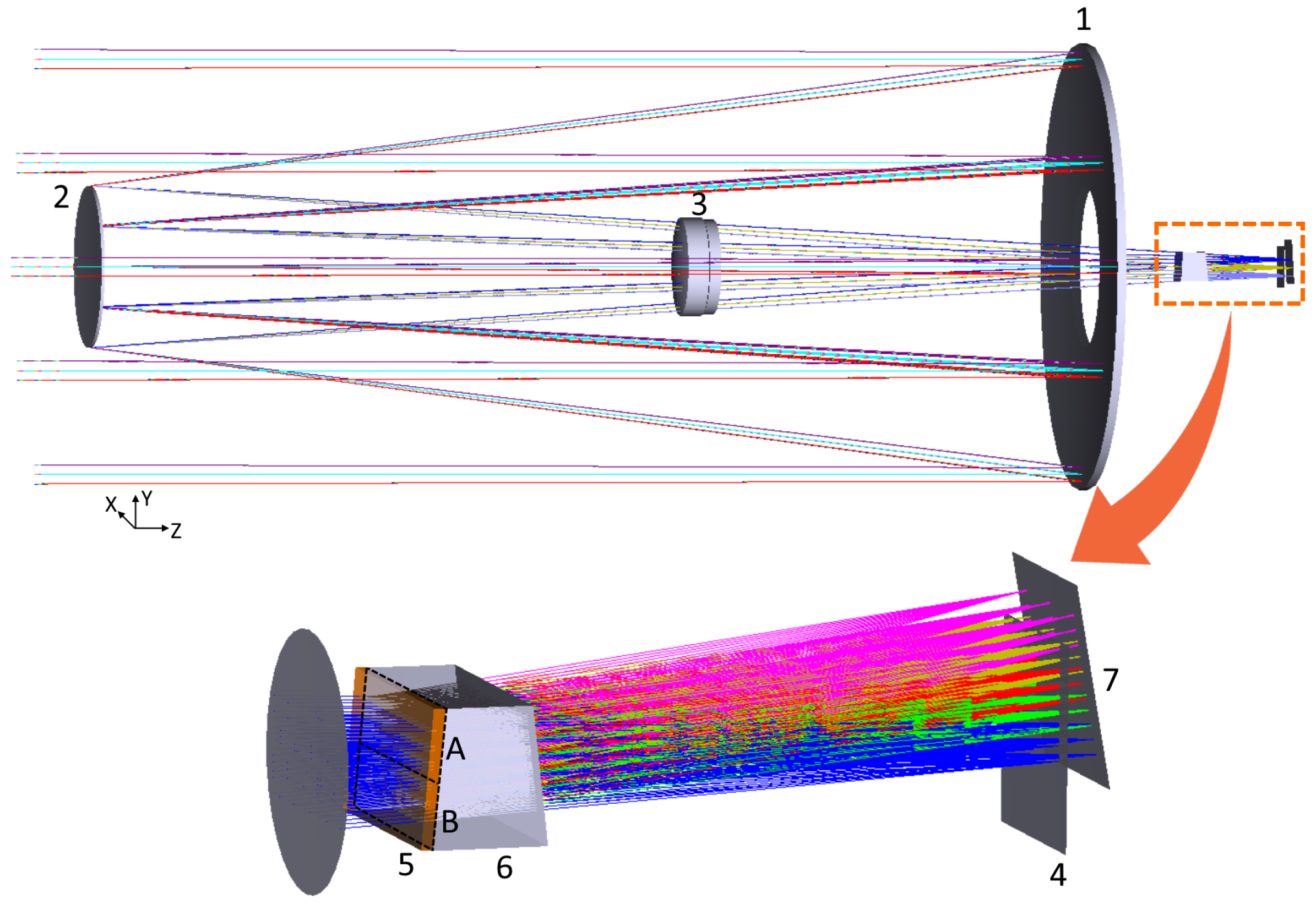
Considering the basic Dall–Kirkham design [13], we can restore a presumable optical layout of the CDK500 and design a slitless spectrograph coupled to it (see Figure 1). The main optical system of the telescope, consisting of the primary and secondary mirrors (1, 2, resp.) and lens corrector 3, forms a converging beam which is focused on the nominal focal plane 4. The grism is mounted in a pre-focal position. It represents a transmission VPH grating 5, recorded on a 3 mm-thick substrate made of $LZO{S}^{TM}$ (Lytkarino, Russian Federation) LK7 glass and glued together with a prism 6. The composite grating represents a mosaiced element consisting of a few rectangular parts, hereafter called zones. The number of zones and their sizes change for different design versions. In practice, the zones can be formed by imposing the photosensitive layer and recording the fringes pattern consequently through a few masks on the same substrate. It was demonstrated that parts of a mosaiced VPH can be co-aligned with high precision and act as a single dispersive element in an astronomical spectrograph [14]. We propose to introduce additional degrees of freedom in the current design, defined for each of the zones separately. The prism is made of $LZO{S}^{TM}$ TK8 glass with an axial thickness of 25 mm and its facets having tilt angles of 4.47${}^{\circ }$ and 6.85${}^{\circ }$ with respect to the telescope optical axis. These parameters are constant for all the design versions discussed below to facilitate the comparison. Note that a solution with a single prism does not allow the creation of an exact zero-deviation geometry, but makes the component much simpler in manufacturing while the deviation angle is moderated. The spectral image is detected by the same CCD array mounted in position 7.

The telescope provides nearly diffraction-limited image quality across the entire FoV and an almost telecentric output beam with the exit pupil position at −1419 mm. For these reasons, we exclude the telescope system from the model and replace it by a perfect lens with the same field and aperture.

As can be seen in Figure 1, adding the spectrograph does not significantly change the telescope’s overall dimensions, and the optical design includes only one optical component. The key functionality is performed by the VPH grating and we consider the following versions of that:

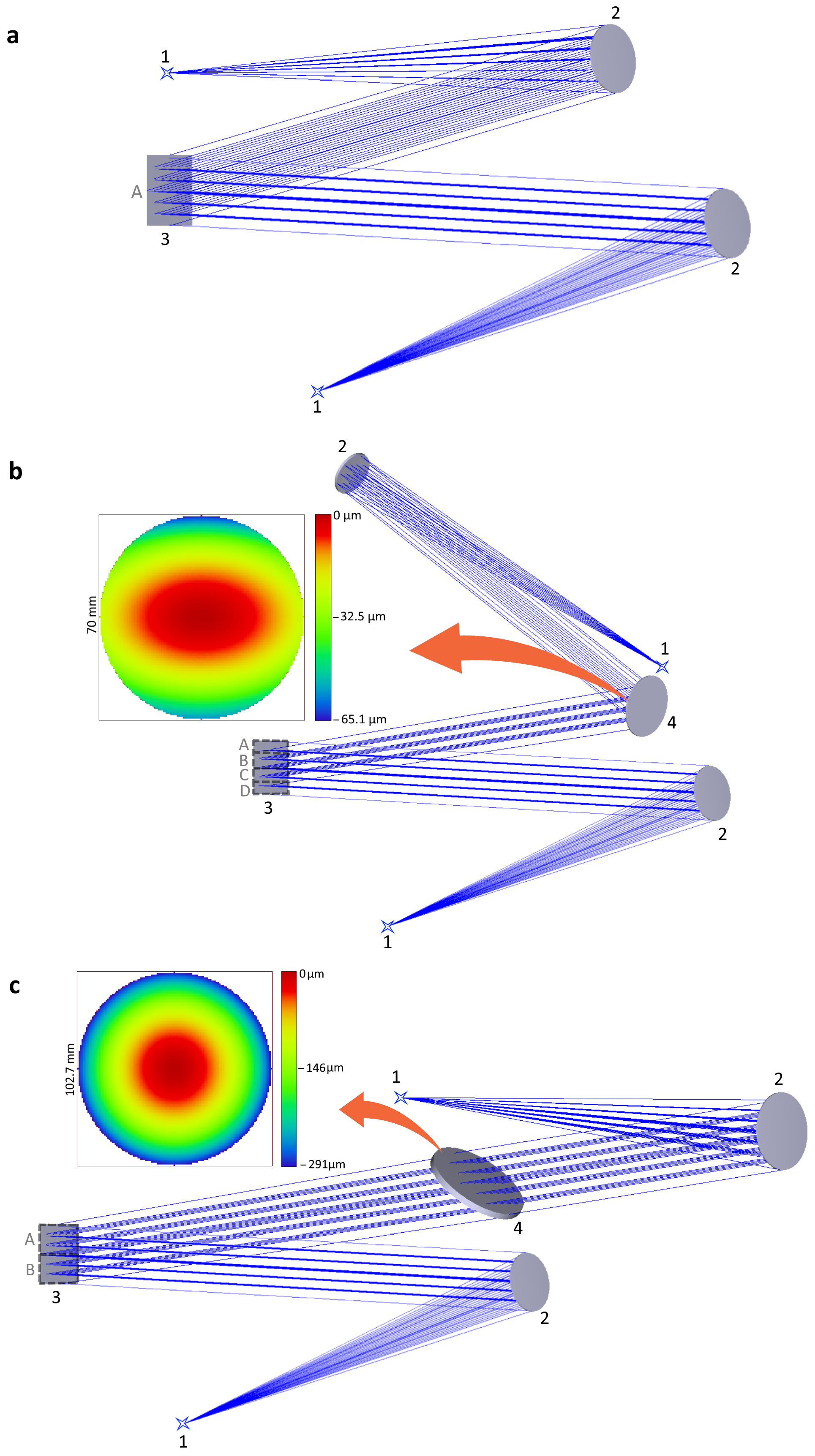
• Classical grating. This is a default option, which can be produced by most manufacturers or even found as an off-the-shelf component. It represents a grating with straight equidistant fringes having a profile perpendicular to the substrate surface. Such a grating can be recorded in a setup shown in Figure 2a, where the laser beam forms two sources 1 and the beams are collimated by two off-axis parabolic (OAP) mirrors 2, which interfere in a symmetric geometry on the substrate 3. The holographic layer thickness is equal to a standard value and the modulation depth is optimized for a chief ray using scalar diffraction theory.
• Composite grating. This version represents all the capacities of the concept shown in [11]. The recording beams in this setup Figure 2b are formed by the same sources 1 and OAP’s 2, but the angles of incidence onto the substrate 3 are not symmetric. A deformable mirror (DM) 4 is introduced in one of the interferometer’s branches to control the wavefront and introduce the aberration correction. The mirror surface shape is described by the Zernike polynomials [15] up to the 2nd order (we use only the YZ-symmetric terms):

  $$z=\frac{r^2/R}{1+\sqrt{1-(1+k)r^2/R^2}}+\sum _{i=4}^{25}{A}_i{Z}_i(\rho ,\varphi );$$

  (1)

  where R, mm is the vertex radius of curvature, k is the conic constant, $Z_i$ are Zernike polynomials, and $A_i$ are corresponding coefficients, r, mm is radial coordinate and $(\rho ,\varphi )$ are normalized polar coordinates of a point on a surface. We presume that the grating is split into four equal horizontal stripes and the deformable mirror shape is optimized for every stripe independently, whereas the rest of the setup arrangement remains the same. In addition to this, we assume that the thickness of the deposed photosensitive layer can be chosen for the stripes independently as well as the exposure time, which defines the index modulation depth. The latter condition can be relatively easily implemented if the grating is recorded through a movable rectangular mask.
• Simplified composite grating. Producing a recording setup as described in the previous item, with all its degrees of freedom, may be very challenging. Therefore, we consider a simplified version. In this setup, the aberrated wavefront is formed by a tilted corrector plate 4 with an ordinary axisymmetric asphere on its first surface:

  $$z=\frac{r^2/R}{1+\sqrt{1-(1+k)r^2/R^2}}+{\alpha }_2{r}^2+{\alpha }_4{r}^4,$$

  (2)

  where ${\alpha }_2$, mm${}^{-1}$ and ${\alpha }_4$, mm${}^{-3}$ are the asphericity coefficients. In this case, we use only two rectangular zones, and the corresponding corrector plates are substituted during the recording. The rest of the recording setup remains the same, including the branches’ asymmetry. Finally, we assume that the thickness of the hologram structure is fixed and equal to a standard value, whereas the modulation depth can be optimized separately for each zone.

We consider the classical grating as a good reference case, since the majority of dispersive units in spectral instruments is represented by such elements and it would be easy to produce and test in practice. The composite element corresponding to Figure 2b is intended to show the capabilities of the proposed solution in terms of image quality and diffraction efficiency improvement once all the currently available technological facilities are employed. The simplified version shown in Figure 2c may be used for early experimental proof of concept since it does not require the use of customized photosensitive layers or active optics. In each case, the recording geometry directly defines the fringes’ shapes and their section profiles, so it should be directly included in the modeling and optimization process. In the following sections, we show the optimization and analyze the performance of each of the presented design options.

3. Image Quality Optimization and Analysis

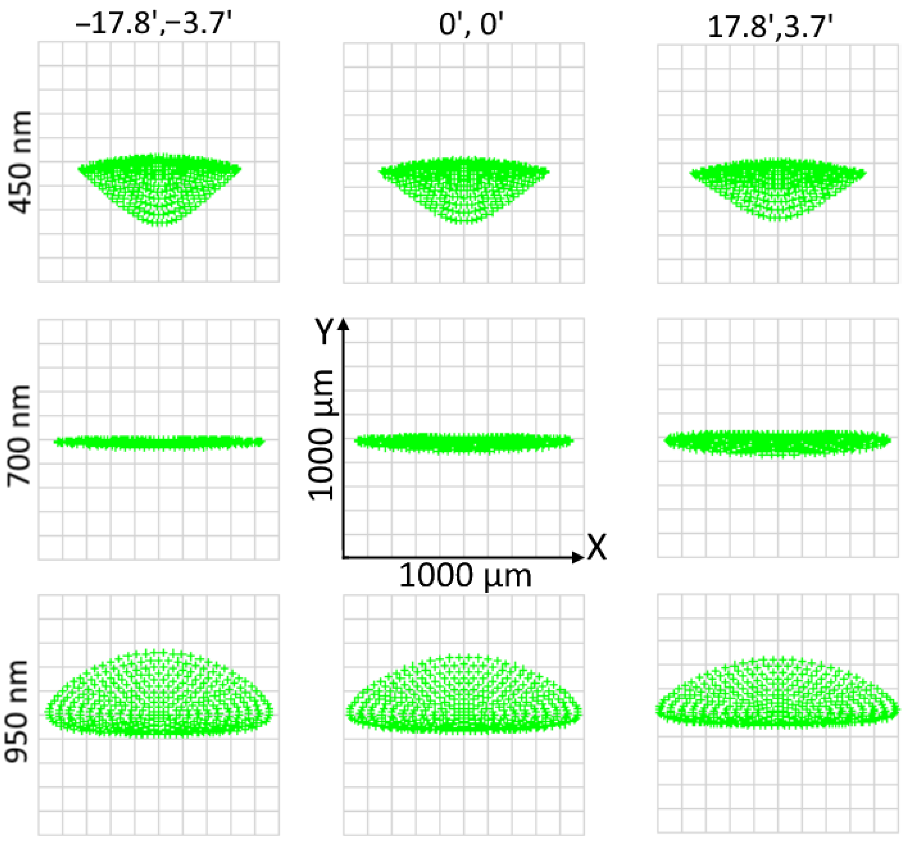
The primary tool used to assess the spectrograph’s image quality is spot diagrams obtained by ray tracing a set of control wavelengths and FoV points. The diagrams for the classical grism are shown in Figure 3, where the X axis corresponds to the spatial direction and the Y axis to the spectral dimension. Note that the optical design is symmetrical with respect to the tangential (ZY) plane and the aberrations vary gradually across the FoV and spectral range. The spot diagrams corresponding to the center and four corners of the FoV at three reference wavelengths characterize the image quality across the entire spectral image. It is assumed that the detector plane is perfectly aligned in its nominal position. It is clear from the plots that the classical grism introduces large aberrations, mainly astigmatism. These cannot be corrected because of a lack of free design variables. In this case, we can only find a focal plane position that minimizes the spot size in the dispersion direction for the central wavelength and a tilt angle for which the spots’ blurring is moderated at the edges of the spectral range. With the given aberrations the spectra of neighboring objects may intersect, limiting the number of simultaneously observable targets drastically. A positive aspect is that the image quality remains relatively stable across the FoV, slightly simplifying the task of aberration correction.

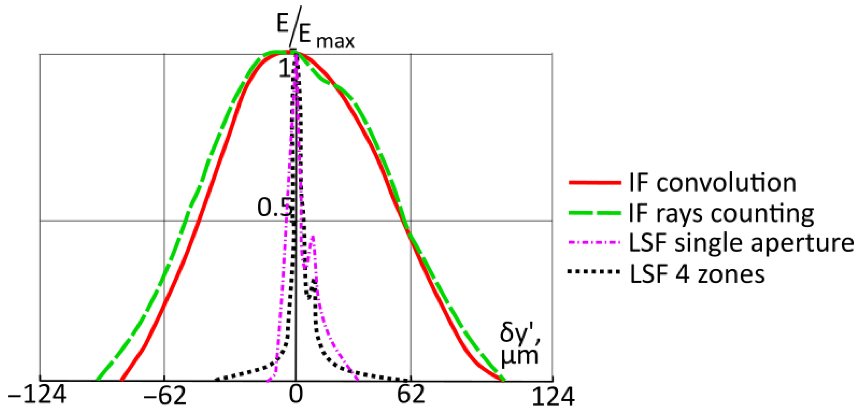
In addition to the spot diagrams, we use instrument functions (IF). An IF represents a transverse illumination distribution in an image of a slit of finite width, or that of a middle section of a finite-size spot image. By definition, this distribution can be obtained as a convolution of the object luminosity function and the optical system line spread function (LSF). This approach works for the classical grism, but not for a composite one, since the LSF is usually computed using a Fourier transform, which ignores splitting of the grating into independent zones. Therefore, for this work, we had to use another, more straightforward method as described in [16]. It relies on tracing a large number of rays covering the full system aperture and the full object width and counting ray intercepts in a number of narrow stripes at the image plane. This technique was used in the past for the IF computation of spectrographs with aberration-corrected holographic gratings and has shown a good match with experimental data [17]. Before applying it for analysis and optimization of the current design, we performed a comparison and verification. In Figure 4, we show two IF plots computed at 700 nm for the FoV center in the case of a single holographic grating—which is not split into zones—computed with two methods. In both computations, we assume that the object luminosity represents a rectangular function with a width of 59 $\mathsf{\mu }$m, which corresponds to 3.5${}^{″}$ seeing. The first curve is computed using a fast Fourier transform (FFT) LSF and the rectangular function. The second one employs the rays-counting approach described above. As one can see, the curves are very similar, with a deviation of $8.6\%$ in width, indicating that the two methods converge well. To illustrate the effects of seeing, aberrations, and the grating mosaicing, we also show the initial LSFs in the same axes. We consider two cases: a single rectangular aperture and an aperture split into four identical rectangular zones. The second case corresponds approximately to Figure 2b but neglects the difference in aberrations for the zones. The zones are separated by thin opaque border lines, corresponding to possible defects at the edges of the recording masks. To emphasize the difference, we set the lines’ width equal to 1 mm. Even with these exaggerated borders’ widths, the LSFs are almost identical. Part of the energy of the LSF peak is diffracted to its wings, but the overall shape and width remain almost the same. Thus, we can conclude that the actual instrument function shape will be driven by the object width, i.e., the seeing, and affected by the optical system aberrations, whereas the influence of diffraction at the apertures is negligibly small.

This technique allows to account for different zones by introducing vignetting and switching between the optical system configurations in a loop. Another point, which usually is not considered when analyzing a spectrograph’s performance, is the object luminosity function. For most instruments intended for laboratory applications it is sufficient to represent it as a simple rectangular function. However, for a slitless spectrograph the object represents a spot already blurred by the atmospheric turbulence and the telescope optics, which does not pass any spatial filter, as an entrance slit, optical fiber, or integral-field unit. Therefore, in the analysis below, we use a conservative estimate of 3.5${}^{″}$ seeing, which corresponds to a 59 $\mathsf{\mu }$m spot in the telescope focal plane and consider two cases:

• a rectangular function of the given width

  $$rect\left(y^{\prime }\right)=\left\{\begin{array}{c}1,-b_1^{\prime }/2\le y^{\prime }\le b_1^{\prime }/2,\hfill \\ 0,|y^{\prime }|\ge b_1^{\prime }/2.\hfill \end{array}\right.$$

  (3)

  where $b_1^{\prime }$ is the slit image width, taking into account the magnification.
• a Gaussian distribution with the given width at level of 0.1

  $$\sigma =\sqrt{\frac{-0.5}{ln0.1\prime }}$$

  (4)

  $$G\left(y^{\prime }\right)=e^{-0.5y^{\prime 2}/{\sigma }^2}.$$

  (5)

where $\sigma$ is the Gaussian distribution dispersion.

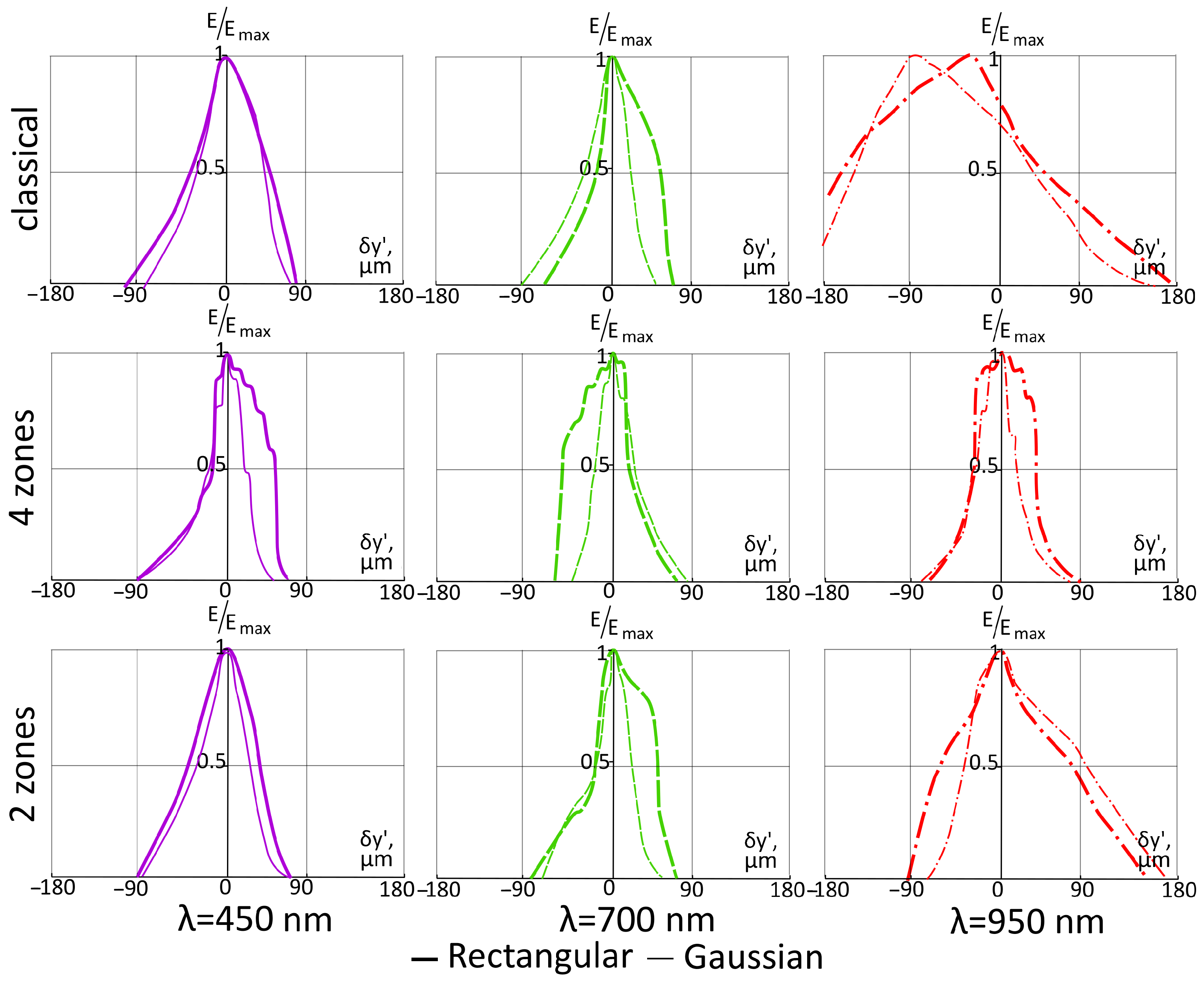
The described computations were implemented as a macro for $ZemaxOpticsStudi{o}^{TM}$ (Ansys, Canonsburg, PA, USA) and shown good convergence with the LSF-based technique for a few test cases. The IFs for the classical grism are shown in a summary comparative diagram in Figure 7. The main outcome of the IFs is their full width at half maximum (FWHM). This value, multiplied by the reciprocal linear dispersion of the spectrograph, gives us its spectral resolution $\delta \lambda$ and from that the spectral resolving power $R=\lambda /\delta \lambda$. All the numerical values, characterizing the spectrograph imaging performances, are shown in a summary in Table 2.

Considering aberration correction, the main difference between the classical grism and the composite ones consists of the presence of a deformable mirror or corrector plates. In the first case, the deformable mirror is mounted with a fixed angle of incidence of 10${}^{\circ }$, 550 mm away from the substrate. Its shape is defined by automated optimization of the root mean square (RMS) spot sizes at the mentioned control wavelengths and FoV points, whereas the aberrations in the spectral direction Y have their weight coefficient increased by a factor of 10 with respect to that for the aberrations in the spatial direction X. Furthermore, the merit function includes boundary conditions, which require maintenance of the image size along the spectral axis, limiting the global Y position of the image edges, the distance between the grism and the detector plane as well as the angle of incidence onto the detector plane at the central wavelength. We may note here that the grating frequency is large enough to keep the zeroth order of diffraction far from the detector, whereas the intensities of higher order diffraction orders for a thick VPH are negligibly low. The resulting profile is dominated by defocusing and astigmatism as can be seen in Figure 2b. The overall deformation of the auxiliary mirror surface found after optimization for the composite hologram is quite large (61–784 $\mathsf{\mu }$m). It can be implemented in practice in two different ways. One approach is to make use of an active thin-shell mirror, similar to that described in [18], which is capable of generating a peak-to-valley (PTV) deformation of 3.4 mm over a 160 mm aperture and create Zernike modes up to and including the 2nd order. This solution is straightforward but requires a customized active component. Another approach is to introduce the dominating defocus mode by re-focusing the collimator and using the DM only for higher modes. In this case, an existing MEMS (micro-electromechanical system)-based DM with a maximum stroke of ≈27 $\mathsf{\mu }$m [19] or even less can introduce the required wavefront deformation. In

Table 1. Optimized parameters of the recording setup.

Zone	Composite		Simplified Composite
	$z_{def}^{\prime }$, mm	$\delta z_{PTV}^{\prime }$, $\mathsf{\mu }$m	$z_{def}^{\prime }$, mm	$\delta z_{PTV}^{\prime }$, $\mathsf{\mu }$m
A	−2168.9	13.7	−3844.8	2.67
B	−3575.9	24.5	−3744.4	2.77
C	−1074.3	22.4	-	-
D	−2984.8	20.9	-	-

we specify separately the beam defocus in millimeters and the PTV deformation of the mirror surface sag corresponding to the rest of the modes (the tip, tilt, and piston are also excluded). In the case of a simplified hologram, the aspheric corrector can be relatively easily polished to the desired surface, but we keep the modes separation to facilitate the comparison. The values indicate that the sag deviation is relatively small, whereas the defocus is large in comparison with the grism size, which is 60 × 34 mm.

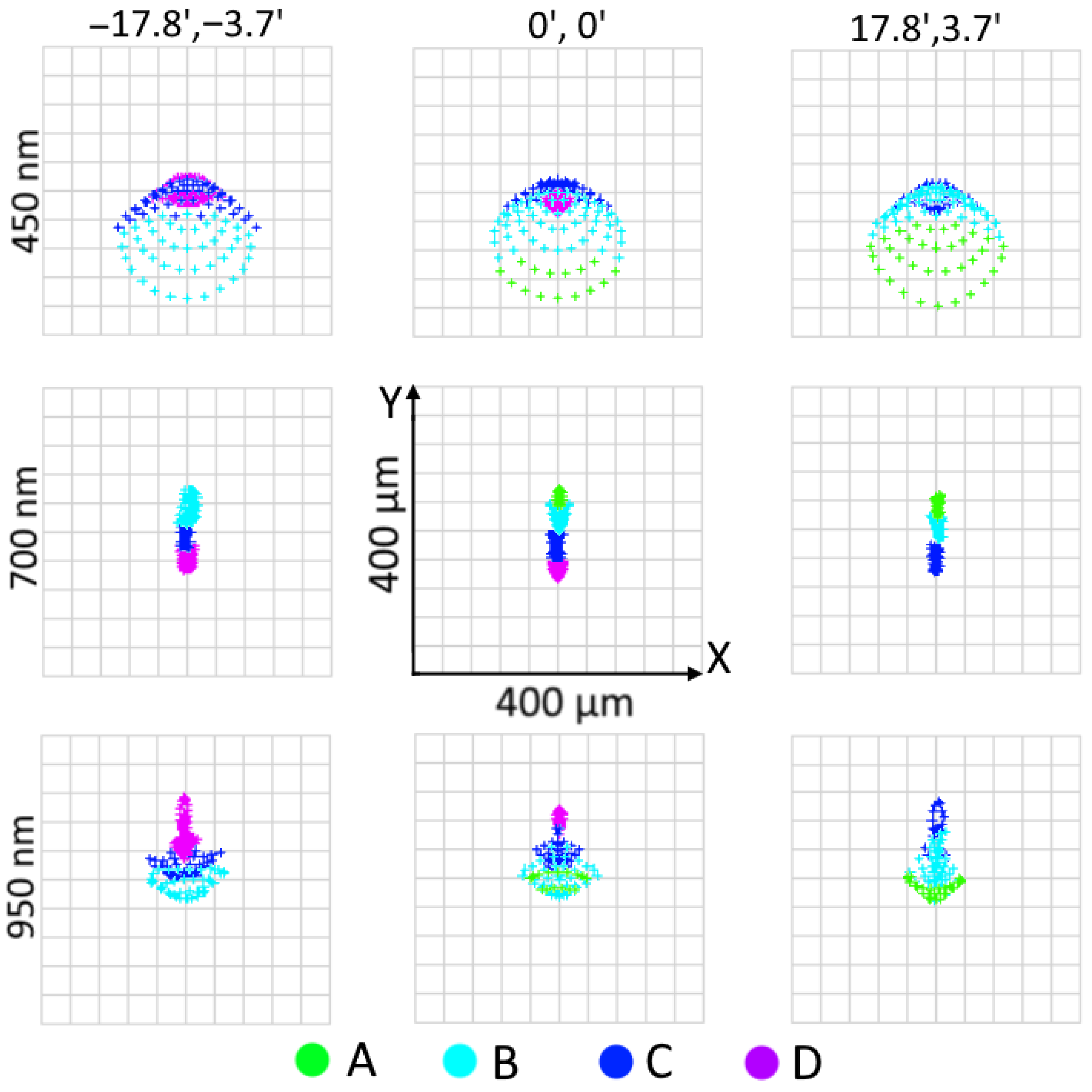
Similarly to the design using a classical grism, we first investigate the spot diagrams—see Figure 5 and

Table 2. Image quality metrics of the slitless spectrograph.

Metric	Classical			Composite			Simplified Composite
Wavelength, nm	450	700	950	450	700	950	450	700	950
FWHM Rect., $\mathsf{\mu }$m	73.4	62.8	208.8	61.3	62	60.8	66.1	63.7	122.4
$\delta \lambda$ Rect.	1.28	1.10	3.64	1.06	0.07	1.05	1.15	1.11	2.13
R Rect., nm	352	639	260	425	654	905	392	632	447
FWHM Gauss., $\mathsf{\mu }$m	61.8	41.4	172.8	35.9	34.8	39.6	49.6	37.8	118.8
$\delta \lambda$ Gauss.	1.08	0.72	3.02	0.62	0.60	0.68	0.86	0.66	2.06
R Gauss., nm	417	967	315	726	1164	1389	523	1067	460
$\delta y_{best}^{\prime }$, $\mathsf{\mu }$m	226	35	223	147	58	95	138	40	128
$\delta x_{best}^{\prime }$, $\mathsf{\mu }$m	309	425	441	74	5	15	61	7	22
$\delta y_{worst}^{\prime }$, $\mathsf{\mu }$m	257	69	259	156	65	114	177	77	170
$\delta x_{worst}^{\prime }$, $\mathsf{\mu }$m	340	457	490	85	9	41	95	27	44

. The diagrams clearly show the contribution of each zone and the gain in the image quality. If we compare the aberrations in the spectral $\delta y^{\prime }$ and spatial $\delta x^{\prime }$ directions, it becomes clear that for the spectral direction at the central wavelength, the aberrations are comparable, whereas at the edges of spectrum, they are reduced by a factor of $2.3$. Meanwhile, the aberrations in the spatial direction are decreased significantly with a gain up to 85 times at the red edge of the spectrum. Therefore, we can expect that the spectra of adjacent objects will be resolved separately and that of extended objects will be free of self-contamination.

The instrument functions of this version of the spectrograph are also shown in Figure 7. They clearly demonstrate the spectral resolution increase for the entire spectrum, but the gain obtained at its long-wavelength edge is very notable. Some high-frequency features can clearly be seen in the plots, which can be attributed to the zone edges. Comparing the numerical values in Table 2 we see that the spectral resolving power growth reaches a factor of $4.4$. It is also notable that the gain is higher by ≈18% compared to the Gaussian distribution assumption. In general, the model predicts a spectral resolving power of up to $R1389$, which is quite high for this class of instruments.

If we step back to the simplified version of the composite grism, the deformable mirror is replaced by two interchangeable corrector plates. Each of them is a 7 mm-thick glass substrate made of $LZO{S}^{TM}$ K8 glass and placed 550 mm away from the hologram substrate. For the zone A recording the tilt angle is 40.604${}^{\circ }$ and for the zone B it is 41.571${}^{\circ }$. The key values, describing the first aspherical surface of each corrector are given in Table 1. Flat aspheres with such parameters are definitely manufacturable.

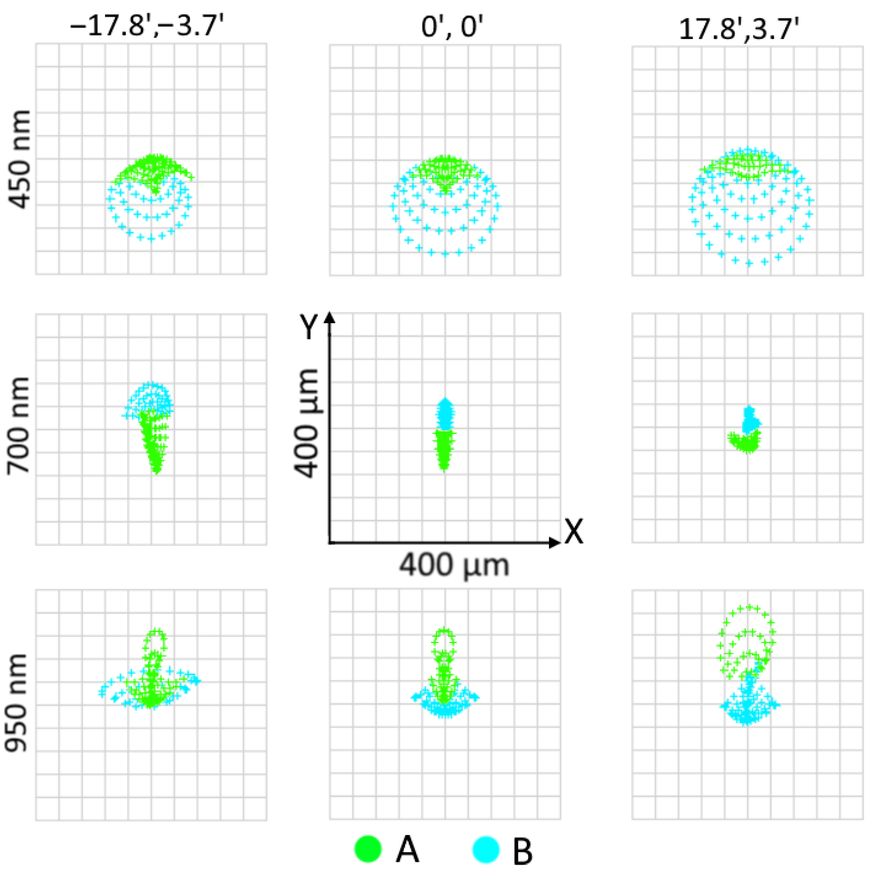
The spot diagrams obtained in this design version are shown in Figure 6. In general, the effect of aberration correction with a composite grism is similar to that seen in Figure 5, although the correction is less uniform across the FoV, and not that efficient at the central wavelength and the red edge. However, in comparison with the classical grism aberrations (Table 2), we still gain a factor of $1.7$ in the spectral direction and $60.7$ in the spatial direction. Thus, the main goal of separating the spectra from different objects can be sufficiently reached even with all the simplifications.

Finally, let us consider the IFs and the spectral resolving power of the simplified grism. The corresponding data are given in Figure 7 and Table 2. Comparing the results with that for a classical grism, one can see that the spectral resolution remains nearly the same at the central wavelength, whereas at the spectrum edges it increases by a factor of 1.12–1.71. The most significant gain is observed for 950 nm with the Gaussian distribution assumption.

In general, both composite grism versions provide good astigmatism correction, which is a key requirement for a slitless spectrograph. This enables the detection of spectral images of multiple objects without intersections and contamination. Furthermore, using auxiliary correcting optics for the grating recording improves the spectral resolving power. If we use four zones of the grating and a deformable mirror, it becomes possible to reach a high and uniform spectral resolution for the entire working range. With two zones and static tilted corrector plates the results are more modest, but the gain at the long-wavelength edge is still significant.

All of the results shown above correspond to the perfect nominal values of the parameters describing the recording and operation setups. In practice, there will be unavoidable errors of manufacturing and assembly. To estimate the tolerances on individual parameters, we perform the following analysis: we introduce small deviations into every parameter p and measure the corresponding change of the weighted RMS of the aberrations over the FoV and aperture at the central wavelength in order to compute the corresponding sensitivity $\partial \sqrt{\sum (w_x{x}^{\prime 2}+w_y{y}^{\prime 2})}/\partial p$. Here, $x^{\prime }$ and $y^{\prime }$ are the transverse aberrations in two directions and $w_x$ and $w_y$ are the corresponding weight coefficients. For a classical grism, we use $w_x=0$ and $w_y=1$, since it has no astigmatism correction, whereas for the composite grisms, we use $w_x=0.1$ and $w_y=1$ as it was during the optimization. Then, presuming the errors for all the S parameters in the system sum up quadratically, we find the individual parameter tolerance as

$$\Delta p=\frac{\Delta \sqrt{\sum (w_x{x}^{\prime 2}+w_y{y}^{\prime 2})}}{\partial \sqrt{\sum (w_x{x}^{\prime 2}+w_y{y}^{\prime 2})}/\partial p}\frac{1}{\sqrt{S}},$$

(6)

where the acceptable change of the aberrations’ RMS is set to $5\%$ of its nominal value.

The computation results are given in

Table 3. Tolerances based on the image quality criterion.

Parameter	Classical	Comp.	Simpl. Comp.
$R_{sub},fr.$	8	8	8
$R_{grat},fr.$	7	8	8
$R_{prism},fr.$	8	8	8
$t_{air}$, mm	0.68	1	1
$t_{grat}$, mm	0.22	0.5	0.5
$t_{prism}$, mm	0.20	0.5	0.5
$d{y}_{grism}$, mm	0.06	0.2	0.2
${\alpha }_{x,grism}{,}^{\circ }$	0.6	1	1
${\alpha }_{y,grism}{,}^{\circ }$	1	1	1
${\alpha }_{x,grat}{,}^{\circ }$	0.013	0.28	0.27
${\alpha }_{y,grat}{,}^{\circ }$	0.26	0.5	0.5
${\alpha }_{x,prism}{,}^{\circ }$	0.023	0.1	0.1
${\alpha }_{y,prism}{,}^{\circ }$	0.94	1	1
$\Delta N_{grat},fr.$	0.52	1	1
$\Delta N_{prism},fr.$	0.52	0.9	0.9
$n_{prism}\times {10}^{-3}$	2.22	1.82	1.76
${\nu }_{prism}$	10	6.1	5.9
$z_{corr}$, mm	-	2	2
${\alpha }_{x,corr}{,}^{\circ }$	-	1	0.3
$t_{corr}$, mm	-	-	0.5
$\Delta N_{corr},fr.$	-	5.7	1.6
$n_{corr}\times {10}^{-3}$	-	-	6.8
$i_{rec}{,}^{\circ }$	0.203	0.145	0.141
$f_{rec}$, mm	-	0.79	0.77

. All the tolerances, which appear to be too wide, are truncated down to a technologically feasible value. The radii of curvature R and irregularities $\Delta N$ are measured in interference fringes at $\lambda$ = 632.8 nm. t denotes the axial thickness. The tip and tilt angles are denoted as ${\alpha }_x$ and ${\alpha }_y$, respectively. n is the index of refraction and $\nu$ is the Abbe number. Note that the latter matters only in the operation setup. $i_{rec}$ is the incidence angle in the recording setup and $f_{rec}$ denotes defocusing of the recording beam. Finally, the indices are as follows: “sub”—grating substrate first surface, “grat”—grating surface, “prism”—second surface of th prism, “grism”—the entire grism, “corr”—the recording wavefront corrector, i.e., the DM or the corrector plate, and “air”—the airgap before the grism.

These values provide approximate estimates of the individual parameter tolerances, but they indicate some notable points regarding manufacturing and alignment:

• Most of the values are feasible to accomplish in practice. It appears that the classical grism is sensitive to decenters and tilts. This can be explained by the large uncompensated aberrations, which grow rapidly when deviating from the found best-fit position. However, the requirements for the individual surfaces’ tilts can be met by defining proper specifications in the drawings of corresponding elements. An angular precision at the level of ≈1${}^{\prime }$ is definitely possible for both the prism and grating.
• The composite grism is more sensitive to the prism refractive properties, but the absolute values are high enough to reach the required precision.
• The simplified version of the composite hologram recording setup does not have wider tolerances for the auxiliary components’ parameters and alignment. The reason for this is that the quality of both surfaces, their position, and material refraction index contribute to the recording of wavefront aberrations.
• The tightest tolerance for a composite gratings’ recording setup corresponds to the corrector plate surface irregularity. However, it should still be technologically feasible.

4. Diffraction Efficiency Optimization and Analysis

Further, we discuss the diffraction efficiency of the grisms in a similar way. As we stated before, it is presumed that the classical grating is recorded in a symmetric setup, so its fringes are perpendicular to the surface. Let us assume that the VPH grating is recorded in dichromated gelatin (DCG) with an Ar laser at a wavelength of 514.5 nm, which is a very typical combination. Then the angles of incidence in the recording setup are 5.087${}^{\circ }$ and −5.087${}^{\circ }$, resulting in a spatial frequency of N = 344.7 mm${}^{-1}$, which corresponds to the required linear dispersion at the image plane. We also assumed that the hologram structure thickness is equal to a standard value of 20 $\mathsf{\mu }$m provided by DCG manufacturers. If all of these parameters are fixed, then the only variable we can use to optimize the DE spectral distribution is the index modulation depth. 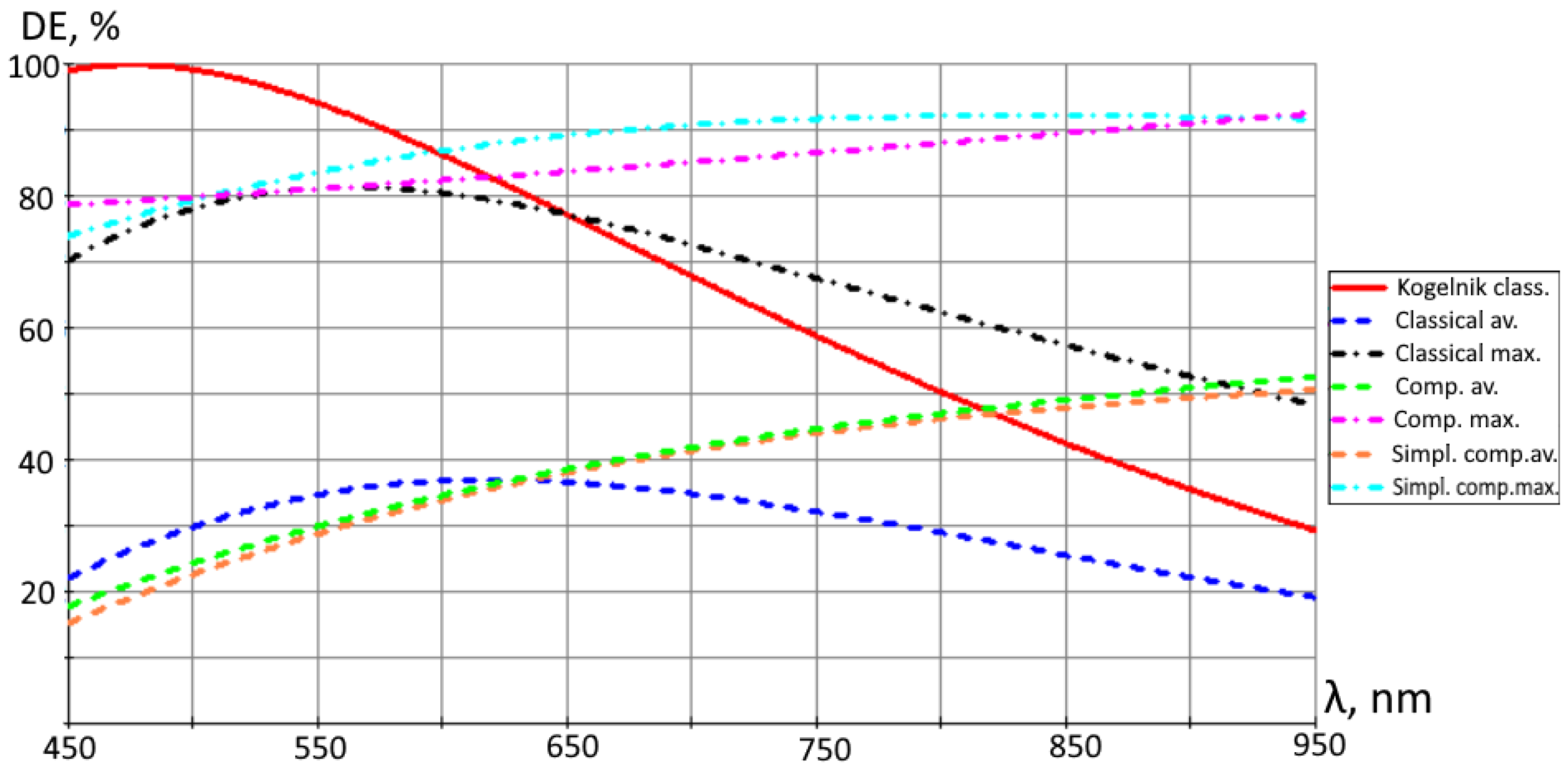We use the analytical equations of Kogelnik’s coupled wave theory [20] to compute the diffraction efficiency and perform this computation in a loop to maximize the sum of DE at five control wavelengths covering the working range uniformly. Note, that we make these calculations only for the FoV center and the chief ray, so the distribution across the field and aperture is ignored. The resulting parameter values are given in the summary table

Table 4. Optimized parameters of the hologram structure.

Zone	Classical		Composite		Simpl. Composite
	t, $\mathsf{\mu }$m	$\delta n$	t, $\mathsf{\mu }$m	$\delta n$	t, $\mathsf{\mu }$m	$\delta n$
A	20.0	0.012	18.5	0.022	20.0	0.019
B	-	-	17.5	0.023	20.0	0.022
C	-	-	22.9	0.018	-	-
D	-	-	20.0	0.028	-	-

and the corresponding DE curve is shown in a comparative plot (Figure 11).

This simplified approach provides us with a starting point and a reference for the hologram structure optimization. However, it is obviously not sufficient to find the best possible design. The grism is mounted in a converging beam and works with an extended FoV; whereas the angle variation across the FoV was shown to be relatively small, the changes across the aperture with $F/\# = 6.8$ are significant. Both the change of the angle of incidence itself and that of the conical diffraction angle take place here. The latter is not taken into account by Kogelnik’s scalar theory. It is necessary that we should use another method to compute the DE precisely. In the present work, we use the rigorous coupled wave analysis (RCWA) [21] implemented in the Reticolo software for these computations. This is a MatLab-based code that computes the diffraction efficiencies and the diffracted amplitudes of gratings composed of stacks of lamellar structures. It incorporates routines for the calculation and visualization of the electromagnetic fields inside and outside the grating. Reticolo implements the RCWA method or frequency–domain modal method for diffraction using 1D structures and is also capable of computing Bloch modes and analyzing stacks of arbitrarily anisotropic multilayered thin films. More details about the RCWA method can be found in [22] and the software description is available at [23].

We use the exact ray tracing results as an input for the diffraction problem to be solved with RCWA across an array of probing points (or elementary gratings), as it was made in [24].

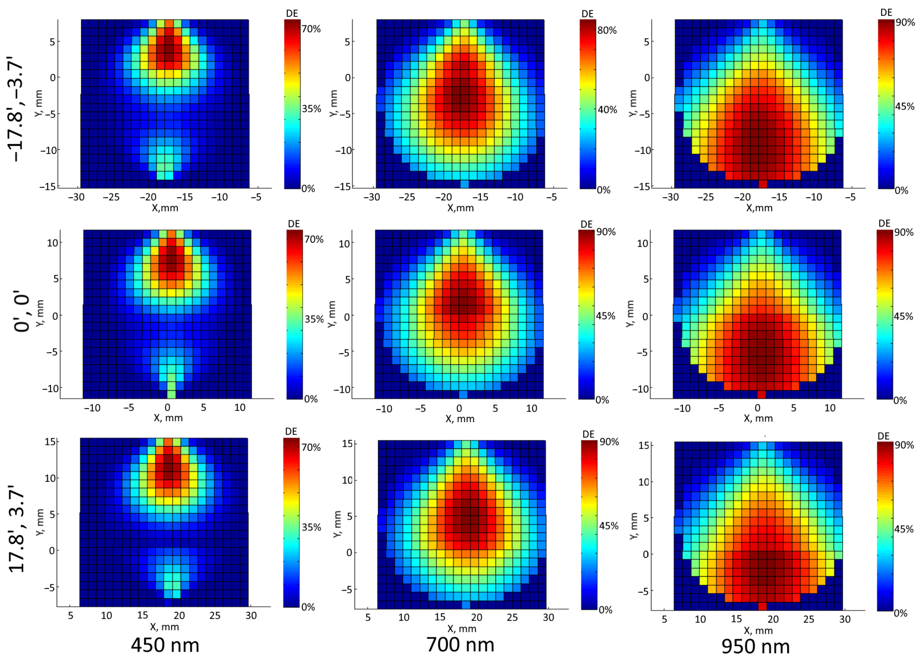
The DE distribution obtained with RCWA for the spectral range center and edges is shown in Figure 8. The corresponding spectral distribution for the FoV center is shown in Figure 11. Note that due to the beam convergence, the DE varies significantly across the aperture, so we plot the average and maximum values in each case separately.

We begin the composite hologram structure design by breaking the recording setup symmetry. We compute the desired fringes’ tilt angle according to the Bragg condition at the central wavelength for the chief ray in the FoV center and obtain angles of incidence of $2.{533}^{\circ }$ and $-7.{141}^{\circ }$. We keep these values fixed whilst performing an automated search of the thickness and modulation depth values to minimize the following function:

$$f(t,\delta n)=\sum _{{\omega }_x=-17.8^{\prime }}^{17.8^{\prime }}\sum _{{\omega }_y=-3.7^{\prime }}^{3.7^{\prime }}\sum _{\lambda =450\mathrm{nm}}^{950\mathrm{nm}}1-{\eta }_{av}(t,\delta n),$$

(7)

here t is the VPH thickness, $\delta n$ is the index modulation depth, and each of them represents a vector of four elements for the A-D zones; $({\omega }_x,{\omega }_y)$ are the angular coordinates of the point in the FoV and ${\eta }_{av}$ is the average DE across the aperture including all the zones of composite grating.

We use a standard simplex method [25] to minimize this function. Since the achievable values of the hologram structure parameters have some technological limits, we apply the following boundary conditions typical for DCG [26]: 10 $\mathsf{\mu }$m $\le t\le$ 30 $\mathsf{\mu }$m and $0.005\le \delta n\le 0.05$.

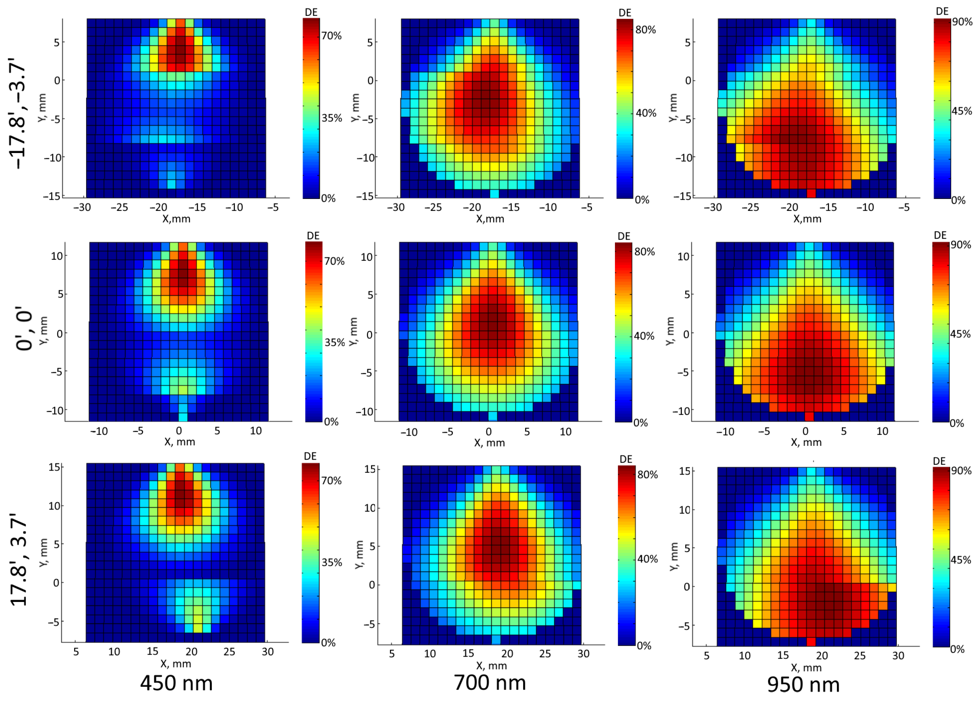
The optimized parameter values are given in Table 4 and the DE distributions are shown in Figure 9. Note that in this case we plot data for points covering the entire FoV since the zone coverage differs across it. One can see that the distribution is more uniform and the values at the red edge are notably higher. Furthermore, these diagrams carry clear footprints of the zone boundaries. The DE at 450 nm represents an illustrative example of the composite hologram concept—the maximum is shifted to the top side of the grating, but the parameters of the lower zone D are optimized locally to partially compensate for this shift. It is necessary to state here that for the RCWA modeling, we introduce some simplification of the recording geometry. When calculating the recording beams’ incidence angles we take into account only the chief ray incidence and the defocus given in Table 1. This allows us to simplify the calculation significantly and avoid the issue of sampling difference in the recording and operation setups, whereas the recording angle deviation does not exceed $0.{16}^{\circ }$.

Similarly, the spectral distribution for the center is shown in Figure 11. Generally, the main qualitative changes are confirmed, but in order to quantify the gain we propose the following metric:

$$Q=\frac{{\int }_{450\mathrm{nm}}^{950\mathrm{nm}}{\eta }_{av}\left(\lambda \right)}{{\int }_{450\mathrm{nm}}^{950\mathrm{nm}}rect\left(\lambda \right)},$$

(8)

i.e., how much energy is diffracted into the working spectral order on average in comparison with an ideal $100\%$ case. After evaluation, the composite grism provides $Q=0.396$, whereas the classical grism had $Q=0.303$. All the values of the Q metrics are summarized in

Table 5. Integral diffraction efficiency metrics.

Field	Classical		Composite		Simpl. Composite
	max	av	max	av	max	av
$-17.8^{\prime },-3.7^{\prime }$	0.690	0.303	0.843	0.383	0.846	0.394
$0^{\prime },0^{\prime }$	0.690	0.303	0.881	0.386	0.853	0.396
$17.8^{\prime },3.7^{\prime }$	0.690	0.303	0.878	0.387	0.845	0.386

. On top of these, we see a very notable increase in the maximum DE.

Next, we perform a similar optimization and analysis for the simplified composite grism. In this case, the hologram thickness is fixed and set equal to 20 $\mathsf{\mu }$m and the hologram consists only of two zones. Therefore, the number of free optimization variables is limited to just two modulation depth values. It would not be enough to provide correction for the entire field of view, so Equation (7) is rewritten for only the FoV center:

$$f^{*}(t,\delta n)=\sum _{\lambda =450nm}^{950nm}1-{\eta }_{av}(t,\delta n),$$

(9)

We minimize this function using the same method and the same boundary conditions and obtain the values listed in Table 4.

The corresponding DE distributions are given in Figure 10. The general distribution patterns are the same, so in comparison with the classical grism, we obtain a more uniform distribution with a better performance at the long-wavelength edge, whereas the specific features of the composite grating are used to recompensate the DE losses at the short-wavelength edge.

The spectral dependencies of the average and maximum DE for the simplified composite grism are shown on the comparative plot Figure 11 together with the other designs. Here the maximum and average values are computed across the beam footprint, i.e., the 2D distribution in every sub-plot in Figure 8, Figure 9 and Figure 10. One can see that despite the simplifications, the performance is superior to that of a classical grism and very close to the case of the initial composite element. We can confirm this using the metric according to Equation (8): $Q=0.386$. From this, it can be seen that in terms of the DE improvement, further complication of the design brings little gain. One possible explanation for this is the grism position. It is located far from the focal and pupil planes, so beams corresponding to different FoV points and aperture parts are mixed, which limits the efficiency of local parameter optimization.

In general, the use of a composite grism will allow us to obtain brighter spectral images and improve the instrument sensitivity, especially in the red part of the spectrum.

Similar to the image quality analysis, we estimate the tolerances for the parameters which define the diffraction efficiency. We use the median value of DE over the working spectral range measured at the FoV center ${\eta }_m$ as the merit function and assume that its acceptable change is $\Delta {\eta }_m=5\%$ in the absolute DE value. Then, we use the following relation, similar to Equation (6):

$$\Delta p=\frac{\Delta {\eta }_m}{\partial {\eta }_m/\partial p}\frac{1}{\sqrt{S}},$$

(10)

In this case, we only consider the hologram structure thickness t, its index modulation depth $\delta n$, and incidence angles in the recording setup $i_{r}ec1$ and $i_{r}ec2$. Even for the slanted fringes, the influence of the two incidence angles on the DE is almost identical. Furthermore, both the frequency and tilt of the fringes change with incident angle deviation. The sensitivity of the DE to the fringes tilt angle change is an order of magnitude higher, so we use the values derived from the fringes tilt angle. All the tolerance estimates are summarized below in

Table 6. Tolerances based on the diffraction efficiency criterion.

Parameter	Classical	Comp.	Simpl. Comp.
$i_{rec}$, deg	0.082	0.046	0.067
t, $\mathsf{\mu }$m	1.6	0.9	1.3
$\delta n\times {10}^{-4}$	6.3	3.5	5.1

.

The values in Table 6 are only estimates, but they indicate a high sensitivity of the DE to the hologram structure parameters. The tolerances on recording angles are tighter than those found with the image quality criterion, but remain at a feasible level >2${}^{\prime }$. The tolerance on thickness is relatively wide—for a 20 $\mathsf{\mu }$m layer a $4\%$ change appears to be acceptable. The highest sensitivity was found for the index modulation depth, but even in the worst case, the tolerance is $2.9\%$. Finally, we can note that the increase of the design variable number obviously causes some tightening of the tolerances, but the difference is moderate.

5. Discussion

The analysis presented above demonstrates that the developed designs of slitless spectrographs based on composite grisms exhibit a clear and measurable gain in performance in terms of both resolution and throughput. Furthermore, these designs, especially the simplified one, are feasible and can be used in the future for an experimental proof-of-concept. From the standpoints of design technique and holographic technology, it introduces some novelty to the field since, to the best of our knowledge, the holographic gratings used in astronomical spectrographs so far could be split into sub-zones [14,27], but did not have local optimization of both aberrations and diffraction efficiency at the same time. However, besides being a demonstrative design, the proposed spectrograph can take its own niche among the astronomical instruments and be useful for real observations. Once we have the numerical estimates of the key performance metrics, it would be useful to compare them with those of some other instruments in order to show the most prospective application areas and the key advantages.

There are a few low-resolution spectrographs working with large ground-based telescopes. They use VPH-based grisms as dispersive elements and operate over an extended field of view. FOCAS [28] and EFOCS [29] can serve as examples. These instruments also try to cover the entire waveband available with a standard CCD detector and utilize the entire field provided by the telescope. The field of view in these cases is smaller than in the proposed design whilst the resolving power and the throughput is comparable or higher than the values we obtained. However, there are notable differences in the optical architectures. In contrast to our design, these spectrographs still use some spatial filters like multi-slit setups in the focal plane and then use auxiliary relay optics and interchangeable dispersers to form the spectral image. This also implies the use of a dedicated detector for the spectral images. Thus, our spectrograph also can be used for observations to take spectra of multiple or extended faint objects. On the one hand, the maximum observable magnitude will be relatively modest, taking into account the difference in collecting area between the telescopes and the optical system transmission. On the other hand, the proposed instrument will benefit from observing a notably larger FoV and the entire waveband at once, whereas its design is much simpler, more compact, and less expensive. The key parameters of the optical designs are compared in

Table 7. Spectrograph characteristics comparison.

Instrument	Comp. Grism	FOCAS	EFOCS	MAO	AFA	Galex-NUV
Wavelengths	450–950 nm	365–900 nm	350–1000 nm	400–1000 nm	350–700 nm	177–283 nm
Spectral resolving power	R425–905	R250–2000	R250–7140	R100	R103–147	R90
Throughput	18–51%	57–82%	18–65%	25–75%	25–75%	10–82%
FoV	35.6${}^{\prime }$ × 7.2${}^{\prime }$	6${}^{\prime }$ × 6${}^{\prime }$	3.5${}^{\prime }$ × 5.7${}^{\prime }$	10.8${}^{\prime }$ × 10.8${}^{\prime }$	14${}^{\prime }$ × 14${}^{\prime }$	⌀1.24${}^{\circ }$
Number of elements	1	15	7	1	1	2
Hosting telescope	CDK500	Subaru	ESO	Zeiss-600	DFM	Galex
	0.5 m ground	8.2 m ground	3.6 m ground	0.6 m ground	0.4 m ground	0.5 m space

.

Another group of instruments that could be compared with our design consists of single-grating slitless spectrographs for small ground-based telescopes. For instance, such an instrument was built at MAO NASU [7,30] for the detection of multiple stellar spectra in a single observation and flare star observations. A similar setup was developed at US AFA [31] and used for the detection of spectra of geosynchronous satellites. In both of these cases, the spectrographs are based on a single transmission grating mounted in a converging telescope beam. Their main parameters are also shown in Table 7. As one can see, the proposed design has a larger FoV and the spectral resolving power is notably higher. For the indicated cases, there are no exact values of transmission available, so we assume that it is close to that of a typical commercial grating [32]. Even with this optimistic assumption, our design shows a comparable performance. This comparison is useful not only to demonstrate the advantages in performance but also to indicate potential applications such as flare star search and spectral characterization as well as the observations of satellites or space debris.

Finally, the developed design can be compared to some space instruments. It is difficult to find a direct analog, but the Galex-NUV channel [6] has a very similar optical design. In comparison with it, our design has a wider working range, higher spectral resolution, and higher minimum throughput. We believe that these advantages can be at least partially maintained if we repeat a composite grism-based design for the NUV domain. We keep this example in the comparative table to emphasize the prospects of our solution for space-based spectrographs as more and more projects of spectral instruments for small satellites like [33] appear.

6. Conclusions and Future Work

In the present work, we have demonstrated the advantages of a composite holographic element being applied in a slitless spectrograph design. It allows for the creation of an extremely compact and simple instrument, which can be mounted in a converging beam at the telescope output, and use the nominal CCD camera of the telescope to detect the spectral image. The key advantage of the composite grism is the astigmatism correction, which allows for decreasing the spot diagram elongation by almost two orders of magnitude. This will make it possible to observe spectra from different objects or different points of an extended object without overlapping, thus implementing the key feature of slitless spectroscopy. On top of this, we can increase the spectral resolving power by a factor up to $4.4$ and improve it significantly at the long-wavelength edge of the spectrum.

In addition to this the composite, VPH has a higher diffraction efficiency that is also distributed more uniformly across the spectral range. Thanks to hologram structure parameters optimization, we can increase the average DE value by a factor of $1.31$. One should keep in mind that when the DE defines the flux power directed to the working diffraction order, the aberrations correction decreases the area in which this flux is focused. Thus, we expect a very significant increase in the spectral image illumination and, therefore, the overall sensitivity of the instrument.

We have considered two versions of the composite grism. The modeling has shown that even with some simplifications, like decreasing the number of zones, using static corrector plates in the holographic recording setup, and using a standard thickness of the holographic layer, it is still possible to obtain a significant gain in performance. Moreover, in terms of DE optimization, a further complication of the design appears to be unnecessary.

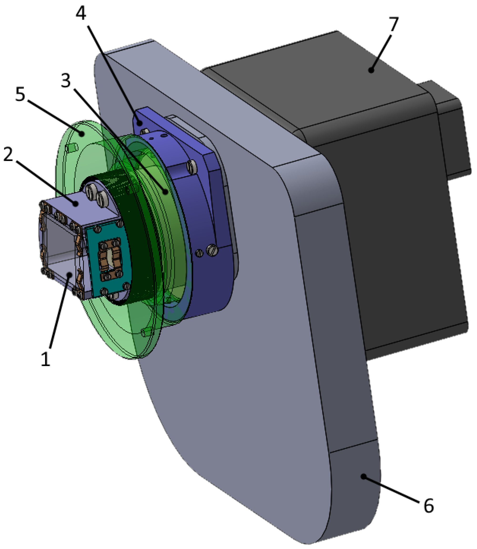
The next stage of our research implies an experimental proof of concept. The plan is to turn the simplified composite grism design into practice and test it experimentally. First, it should be tested in the laboratory, including measurements of the resolution and throughput. Second, we plan to make trial observations with the spectrograph coupled with the CDK500 telescope owned and operated by Kazan Federal Univ. Figure 12 shows the optomechanical design of the slitless spectrograph unit to be mounted on the telescope.

To the best of our knowledge, it would be the first application of a composite holographic dispersion element in an operational astronomical instrument. Thus, it should provide a strong confirmation of the very design concept advantages and to the corresponding design and modeling techniques. We hope that this instrument will open new prospects for spectral instrument design in astronomy and other fields.