Statistical Tool Size Study for Computer-Controlled Optical Surfacing

Abstract

Over the past few decades, computer-controlled optical surfacing (CCOS) systems have become more deterministic. A target surface profile can be predictably achieved with a combination of tools of different sizes. However, deciding the optimal set of tool sizes that will achieve the target residual error in the shortest run time is difficult, and no general guidance has been proposed in the literature. In this paper, we present a computer-assisted study on choosing the proper tool size for a given surface error map. First, we propose that the characteristic frequency ratio (CFR) can be used as a general measure of the correction capability of a tool over a surface map. Second, the performance of different CFRs is quantitatively studied with a computer simulation by applying them to guide the tool size selection for polishing a large number of randomly generated surface maps with similar initial spatial frequencies and root mean square errors. Finally, we find that CFR = 0.75 achieves the most stable trade-off between the total run time and the number of iterations and thus can be used as a general criterion in tool size selection for CCOS processes. To the best of our knowledge, the CFR is the first criterion that ties tool size selection to overall efficiency.

1. Introduction

Computer-controlled optical surfacing (CCOS) [1,2] systems have been successfully used to fabricate high-precision optics in various cutting-edge applications, such as telescopes for space exploration [3,4,5], X-ray mirrors for synchrotron radiation and free-electron laser facilities [6,7,8,9,10], and optics in EUV lithography [11,12]. Different CCOS systems use different tools, which can be adopted based on the requirements for the precision and shape of the desired optical surface.

CCOS uses tools that are much smaller (i.e., sub-aperture tools) than the optical surface to correct the local errors. All CCOS techniques are mathematically modeled and have become much more deterministic [13,14], which enables a desired optical surface to be predictably achieved with a combination of tools with different sizes. In the CCOS process, a tool is simulated by its material removal footprint, known as its tool influence function (TIF). It is well known that certain TIF sizes have limits on the feature sizes within the optical surface that they can correct [2,15,16,17]. Basically, larger TIFs with higher peak removal rates (PRRs) are preferred because they remove material faster. However, while any given TIF can correct features larger than the size of the TIF completely, they cannot correct features that are smaller than the TIF footprint well. On the other hand, if the TIF is too small, then the surfacing efficiency will be low, and unexpected mid-to-high-frequency errors may be left on the optical surface. Therefore, choosing the optimal set of TIF sizes that achieves the target residual surface error with the shortest run time has been a difficult problem in practical CCOS processes. This problem is especially important in the fabrication of large optics, where a small improvement of efficiency leads to a great reduction in manpower and financial resources.

Reducing the fabrication time through more efficient and deterministic computer-controlled grinding, polishing, and metrology will allow larger-aperture space telescopes to be launched since the available budget will extend further [18]. As an example, saving a part of the overall fabrication time and iterative fabrication loops for each of the 798 hexagonal segments of the European Extremely Large Telescope (E-ELT) [19] will save significant time and uncertainties in the overall schedule.

Conventionally, a set of tools was empirically determined by a fabrication artisan’s experience. However, multiple iterations of the trial-and-error cycle are usually required to approach the target residual surface error, which is inefficient. Additionally, this method highly relies on the expertise of the artisan and thus cannot be formalized as a general guidance.

Quantitative characterization of the correction capability of a certain TIF has been attempted by examining the power spectral density (PSD) of the TIF [15,16,17] in the literature. The PSD uses the Fourier transform to decompose a TIF and a surface error map into different spatial frequencies with their respective amplitudes. The amplitudes quantify the contributions of certain spatial frequencies to the entire surface error map. With the help of the PSD, Zhou et al. theoretically analyzed the removal characteristics in the CCOS process using a sinusoidal surface error map that only contained a single spatial frequency. A material removal availability (MRA) value equal to the ratio between the target material removal volume and the actual (or predicted) material volume removed was proposed as an indicator of the correction capability of a particular TIF [15]. The MRA can be used to determine how well a TIF can correct certain spatial frequencies. However, the concept was only verified for individual frequencies, and the relationship between the MRA and the total run time was unclear. Wang et al. presented a procedure for using the PSD to calibrate a specific TIF to determine its capability of correcting features that are smaller than the TIF [16,17]. However, this procedure requires multiple real fabrication runs and metrology to feed back to the result, specifically focusing on the smoothing efficiency of a TIF. Therefore, the method is not generally applicable to other TIFs without running the same procedure.

In this study, we present a computer-assisted analysis of the general guidance to choosing proper tool sizes for a given surface error map. First, the concept of the characteristic frequency ratio (CFR) is developed from Fourier theory and calibrated with a reference single-frequency sinusoidal surface as a proper measure of the correction capability of a certain TIF. Second, the relationship between the CFR and the run time is quantitatively studied via massive computer simulations, where different combinations of CFRs are applied as a reference in choosing the tool sizes for a large number of randomly generated surface error maps with similar initial spatial frequencies and root mean square (RMS) values. The statistics for each CFR combination, including the average of the run time, the standard deviation of the run time, and the number of iterations, are summarized and compared. Finally, the simulation results demonstrate that the CFR of 0.75 achieved the most stable trade-off between the total run time and the number of iterations and thus could be selected as a general efficiency criterion in choosing the tool sizes in CCOS. To the best of our knowledge, this is the first statistical study of tool size selection, and the CFR is the first general criterion that ties the TIF correction capability to the total run time.

The rest of this paper is organized as follows. The necessary background of Fourier theory as applied to analyze surface errors is briefly reviewed in Section 2, followed by a detailed explanation of the novel characteristic frequency (CF) of a TIF and its calibration in Section 3. Section 4 provides examples of determining the CFs for three standard TIF shapes, and then Section 5 describes the proposed CFR criterion. The computer-assisted study of different CFRs is discussed in Section 6, which includes a discussion on the practical applicability and limitations of the study. Section 7 concludes the paper.

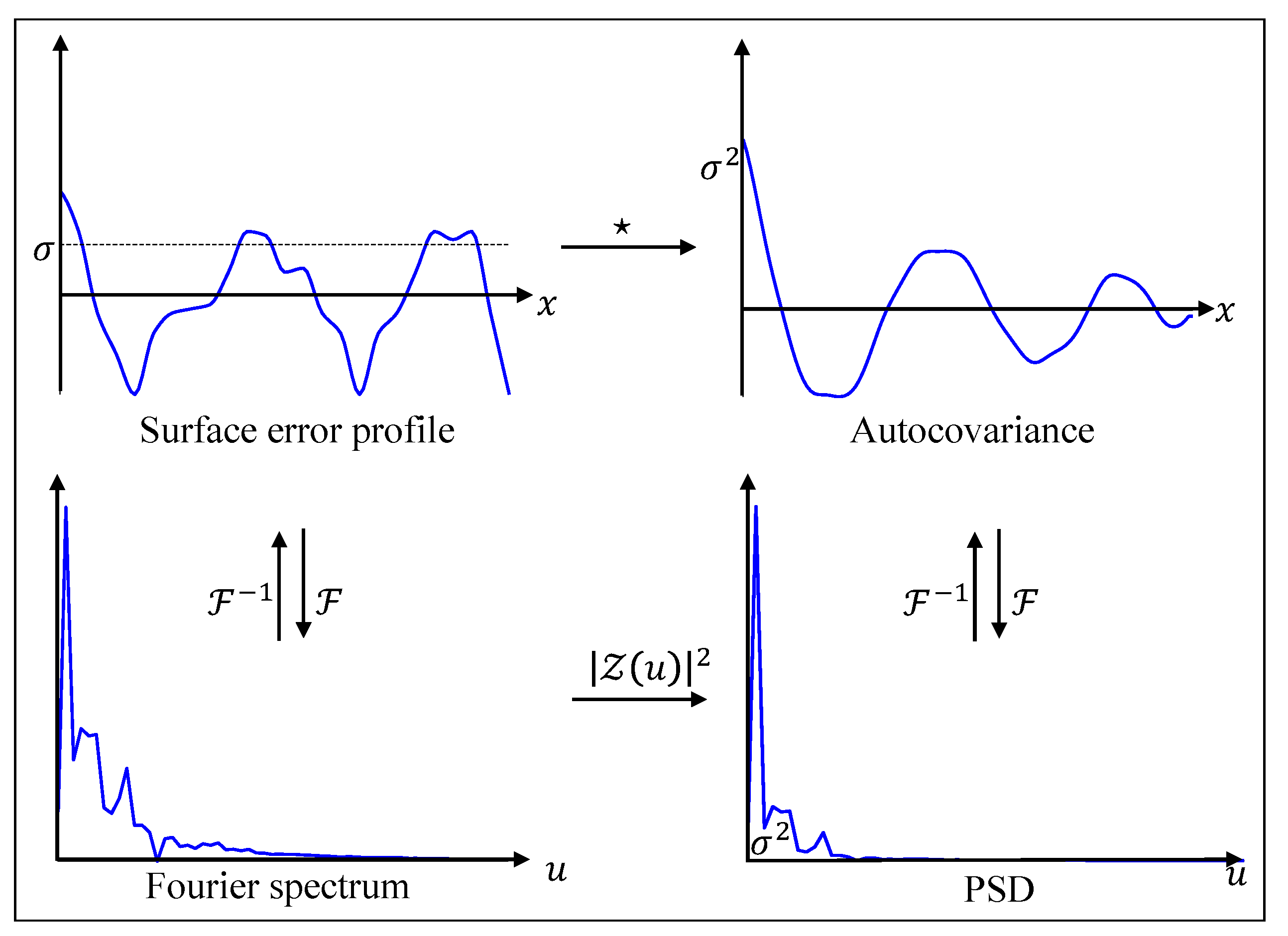
2. Fourier Analysis of Surface Error

2.1. The Fourier Transform

In optical fabrication, surface errors are usually described as a 2D matrix of the difference between the measured and target surface shapes. This surface error map consists of error features which vary in lateral size and magnitude. The discrete Fourier transform (DFT) of the surface error is defined as follows:

$$\mathcal{Z}\left(u,v\right)=l_x{l}_y\sum _{x=0}^{N_x-1}\sum _{y=0}^{N_y-1}Z\left(x,y\right)e^{-i2\pi \left(\frac{u}{N_x}x+\frac{v}{N_y}y\right)},$$

(1)

where $\mathcal{Z}\left(u,v\right)$ is the 2D spatial frequency spectrum of the surface error $Z\left(x,y\right)$ and $l_x\times l_y$ is the pixel size. Here, $l_x=N_x/L_x$ and $l_y=N_y/L_y$, where $N_x$ and $N_y$ are the numbers of sample points in the x and y directions, respectively, and $L_x$ and $L_y$ are the periodicity in the x and y directions, respectively. The DFT decomposes the surface error into all the spatial frequencies which are present in the measurement, represented by sinusoidal features and their respective amplitudes.

2.2. Power Spectral Density

The power spectral density (PSD) of a surface is a statistical tool that decomposes a surface into contributions from different spatial frequencies. Figure 1 illustrates the relationship between the measured surface profile and its one-dimensional PSD curve, namely that the PSD is the Fourier transform of the auto-correlation function of the surface error map, which contains the power across a range of frequencies. An important realization is that the PSD of the mean-removed surface error gives the surface variance of each spatial frequency present in the measurement.

It is worth mentioning that in the real implementation of a DFT defined in Equation (1), it is assumed that $l_x=l_y=1$ so that $1/L_x{L}_y=1/N_x{N}_y$ [20]. Therefore, according to Figure 1, the PSD based on Equation (1) can be calculated as follows:

$$\mathcal{P}\left(u,v\right)=\frac{1}{N_x{N}_y}{\left|\mathcal{Z}\left(u,v\right)\right|}^2.$$

(2)

2.3. Encircled Error

In optical metrology, the encircled energy has been used to measure the concentration of energy of a point spread function (PSF) at the image plane. Analogous to the encircled energy of a PSF, we define the encircled error (EE) of a PSD as follows:

$$E\left(r\right)=\frac{{\displaystyle \sum _{\theta =0}^{2\pi }}{\displaystyle \sum _{\rho =0}^r}\mathcal{P}\left(\rho ,\theta \right)}{{\displaystyle \sum _{\theta =0}^{2\pi }}{\displaystyle \sum _{\rho =0}^{\mathrm{R}}}\mathcal{P}\left(\rho ,\theta \right)},$$

(3)

where $\mathcal{P}\left(\rho ,\theta \right)$ is $\mathcal{P}\left(u,v\right)$ transformed to the polar coordinate system, $\rho$ is the sampled frequency measured radially from the central frequency bin, $\theta$ is the azimuthal angle covering the PSD, and $\mathrm{R}$ is the maximum spatial frequency within the PSD. As an example, Figure 2a shows a randomly generated surface with a total RMS error of 98.8 nm. Figure 2b is its two-dimensional (2D) PSD map, and Figure 2c gives the corresponding EE. Recalling that the PSD of the mean-removed surface error is the surface variance contribution of each spatial frequency contained in the measurement, the EE then reveals what percentage of the error is due to spatial frequencies lower than a given frequency.

2.4. Characteristic Frequency of a Surface Error Map

For an optical image, a typical criterion for the encircled energy is the radius of the PSF at which 50% or 80% of the energy is encircled. As an analogy for this study, we define the characteristic frequency (CF) of a given surface error map to be located at EE = 80% as

$$f_{SURF}^c=\underset{r}{\arg }\left[E\left(r\right)=80\%\right],$$

(4)

where $f_{SURF}^c$ refers to the CF of the surface error map. For example, as shown in Figure 2b,c, the CF of this surface error map is $f_{SURF}^c=3.41$ m${}^{-1}$.

3. The Reference TIF

Zhou, et al. discussed how the amplitude frequency spectrum, given by the Fourier transform of a tool influence function (TIF), is a measure of the correctability of that TIF for localized errors of the same spatial frequencies [15]. We used a reference surface and a reference TIF to calibrate the CF of the TIF.

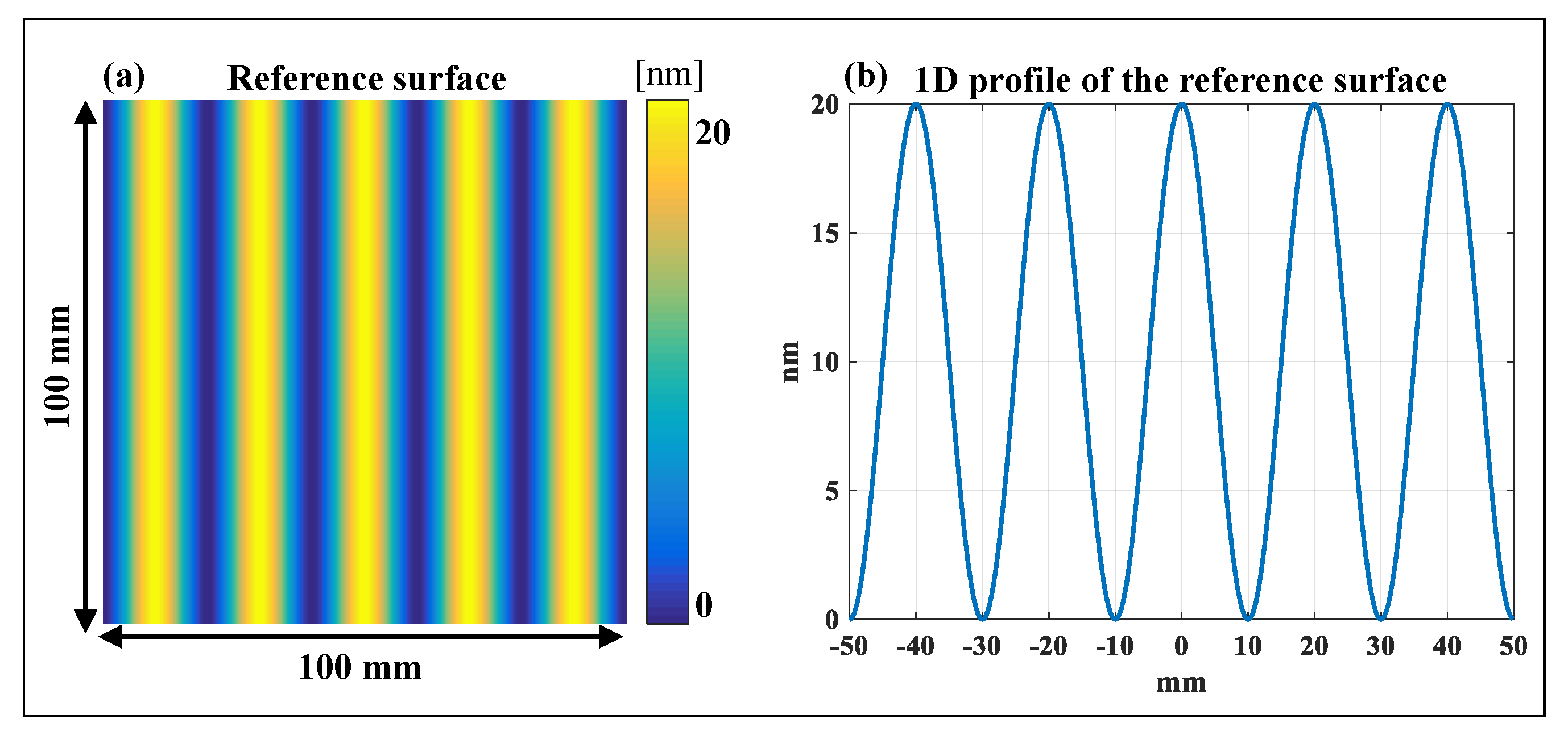
3.1. The Reference Surface

Since the Fourier series decomposes surface errors into sinusoidal patterns, we define a reference surface error map containing a single Fourier mode in the x direction as

$$Z_{REF}\left(x,y\right)=\mathrm{A}·\cos \left(2\pi fx\right)+\mathrm{A},$$

(5)

where A is the amplitude and f is the single spatial frequency of the surface error. The reference surface error map and its profile along the x direction are shown in Figure 3a,b, respectively, where the size of the map is 100 mm × 100 mm, and A = 10 nm and $f=0.05$ mm${}^{-1}$ are used in this study. It is worth mentioning that A and f could be set arbitrarily and not affect the outcome of the analysis. We also note that the surface error was piston-adjusted to have no negative values, since CCOS processes are only capable of removing material.

3.2. Preston’s Equation and the Line TIF

The material removal process is classically defined by Preston’s equation [2] as follows:

$$\frac{\partial Z\left(x,y\right)}{\partial t}=\kappa ·P\left(x,y\right)·V\left(x,y\right)$$

(6)

where the material removal rate per unit time $\partial Z\left(x,y\right)/\partial t$ is proportional to the contact pressure $P\left(x,y\right)$ and the relative velocity $V\left(x,y\right)$ between the tool and the workpiece. Preston’s constant, $\kappa$, is used to consider additional factors that contribute to friction between the tool and the workpiece, such as slurry and polishing interface material. This equation is used to theoretically define a static TIF, which gives the material removal rate of a polishing process if the tool is parked in one spot and allowed to run for one unit of time. According to Equation (6), a TIF which matches the shape of the error feature will perfectly correct that error in the shortest amount of time (i.e., the most efficient TIF for that feature).

The static TIF considers only the motion of the tool without traveling across the workpiece. Many CCOS processes use a spiral tool path, and therefore the Ring TIF was conceived [21]. The Ring TIF considers the motion of tools traveling across the workpiece as the workpiece rotates under the tool and is therefore a function of the radial position from the center of the workpiece. To simplify this technique, we define the Line TIF, which is defined in the same way as the Ring TIF, only a Cartesian raster tool path is assumed rather than a spiral one. Converting the 2D static TIF to the Line TIF is as simple as summing down the columns (or equivalently the rows, depending on the major direction of the raster path) of the static TIF matrix.

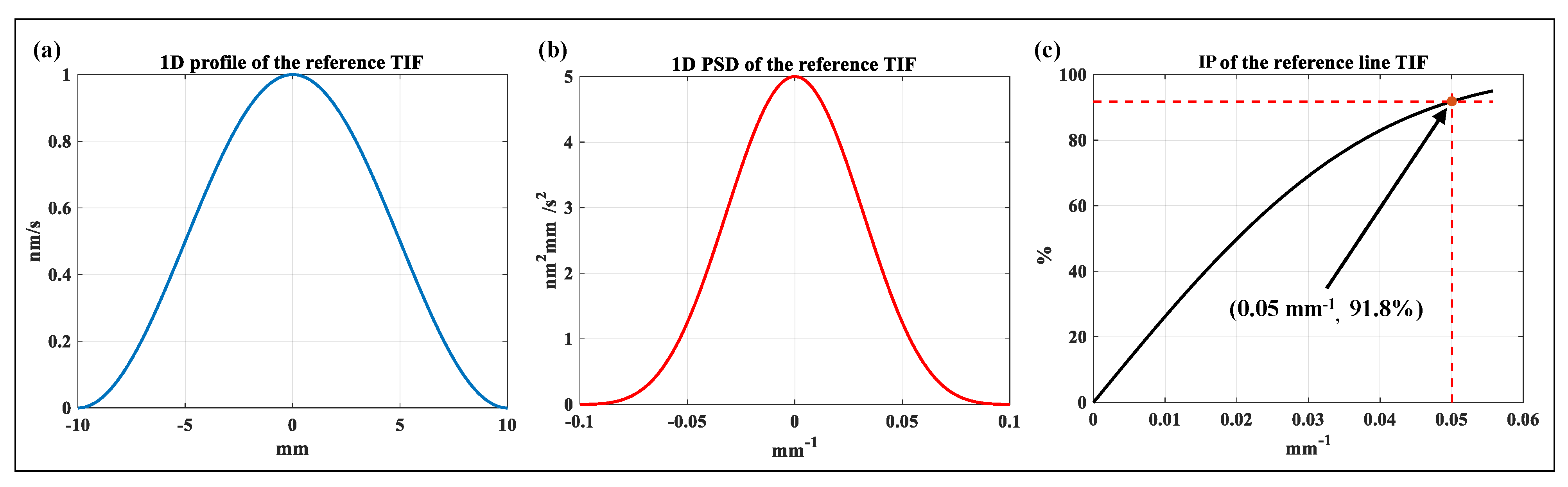
3.3. The Reference TIF

Therefore, the ideal (i.e., reference) Line TIF $I_{REF}\left(x,y\right)$ for the single-frequency surface error map is simply one period of the sinusoid of the same frequency, defined by

$$I_{REF}\left(x,y\right)=\frac{\mathrm{PRR}}{2}·\cos \left(2\pi fx\right)+\frac{\mathrm{PRR}}{2},f=0.05{\mathrm{mm}}^{-1},$$

(7)

where PRR is the peak removal rate of the TIF and the TIF is piston-adjusted by PRR/2 so that there are no negative removal rates. It is obvious from Equations (5) and (7) that the ideal TIF to correct the reference surface in Figure 3 is the sinusoidal reference TIF with a frequency $f=0.05$ mm${}^{-1}$. Therefore, the CF of the reference TIF is defined to be $f_{TIF}^c=0.05$ mm${}^{-1}$. Figure 4a shows the 1D profile of the reference TIF in the x direction with PRR = 1 nm/s.

3.4. Integrated PSD and the Characteristic Frequency of a TIF

To generalize the CF to any TIF, we take the analysis from Zhou et al. further by defining the Integrated PSD (IP) of a TIF to calibrate a TIF’s CF. As shown in Figure 4b,c, the IP is simply a one-dimensional (1D) equivalent of an EE calculation (see Equation (3)) performed on the 1D PSD of the Line TIF. For the reference TIF with $f_{TIF}^c=0.05$ mm${}^{-1}$, as demonstrated in Figure 4c, the corresponding IP occurs at 91.8%. Therefore, we define the CF for any TIF as the spatial frequency where IP = 91.8%; in other words, we have

$$f_{TIF}^c=\underset{r}{\arg }\left[I\left(r\right)=91.8\%\right].$$

(8)

4. Extending the Calibration to Other TIF Shapes

When utilizing the calibration of the $f_{TIF}^c$ (see Equation (8)) by means of the reference TIF illustrated in Section 3.1, we can determine the size of any kind of TIF by simply applying a scale factor, depending on the given TIF shape. In the following subsections, we provide examples that employ Equation (8) to determine the appropriate size of three kinds of typical TIFs in CCOS to correct the reference surface in Figure 3, namely Gaussian TIFs [10], Spin TIFs [22], and Orbital TIFs [22], with the objective that the CF of these TIFs matches the only error frequency present in the reference surface in Section 3.1.

4.1. The Gaussian TIF

The zero-mean, rotationally symmetric Gaussian TIF can be defined as follows:

$$I_G(x,y)=\mathrm{PRR}·\exp \left(\frac{x^2+y^2}{2{\sigma }^2}\right),$$

(9)

where $\sigma$ is the standard deviation of the Gaussian distribution that defines the size of the Gaussian TIF. The size of a Gaussian TIF can be defined by the full width at half maximum (FWHM), defined as $\mathrm{FWHM}=2\sigma \sqrt{2\ln 2}$. Then, the scale factor for the Gaussian TIF is $\mathrm{FWHM}/f_{TIF}^c$.

4.2. The Spin TIF

The Spin TIF is derived from Equation (6) as follows:

$$I_S\left(x,y\right)=\{\begin{array}{ll}\kappa ·P\left(x,y\right)·\omega ·\rho \left(x,y\right),& \rho \le {\mathrm{R}}_T,\\ 0,& \rho >{\mathrm{R}}_T\end{array}$$

(10)

where $\omega$ is the angular velocity of the spinning motion of the machine tool, ${\mathrm{R}}_T$ is the radius of the actual tool, and $\rho (x,y)$ is the radial distance from the center of the tool. The size of the Spin TIF is defined only by the size of the tool such that ${\mathrm{R}}_{TIF}={\mathrm{R}}_T$. The scale factor for the Spin TIF is then ${\mathrm{R}}_{TIF}/f_{TIF}^c$.

4.3. The Orbital TIF

The Orbital TIF is also derived from Equation (6) but is much more complicated than the previous two TIFs. Dong et al. provided a well-organized derivation of the Orbital TIF [23], which is summarized as follows:

$$I_O\left(x,y\right)=\{\begin{array}{ll}\frac{\pi }{30}·\kappa ·P\left(x,y\right),& \rho \le {\mathrm{R}}_T-{\mathrm{R}}_O,\\ \frac{1}{30}·\kappa ·P\left(x,y\right)·\omega ·{\mathrm{R}}_O·arccos\left(\frac{{\rho }^2\left(x,y\right)+{\mathrm{R}}_O^2-{\mathrm{R}}_T^2}{2·\rho \left(x,y\right)·{\mathrm{R}}_O}\right),& {\mathrm{R}}_T-{\mathrm{R}}_O<\rho \le {\mathrm{R}}_T+{\mathrm{R}}_O\\ 0,& \rho >{\mathrm{R}}_T+{\mathrm{R}}_O\end{array}.$$

(11)

where ${\mathrm{R}}_O$ is the radius of the orbital stroke and all the other variables are the same as those presented in Equation (10). Unlike the previous two TIFs, the Orbital TIF is defined by two parameters: ${\mathrm{R}}_T$ and ${\mathrm{R}}_O$, where ${\mathrm{R}}_{TIF}={\mathrm{R}}_O+{\mathrm{R}}_T$. Similar to the Spin TIF, the scale factor for the Orbital TIF is ${\mathrm{R}}_{TIF}/f_{TIF}^c$.

4.4. Determining the TIF Size to Match a Desired CF

In order to determine the desired TIF size for a given CF, we simply generate an arbitrarily sized TIF, calculate the scale factor, and multiply by the desired CF (i.e., $R_{TIF,desired}=R_{TIF,arbitrary}/f_{TIF,arbitrary}^c\ast f_{TIF,desired}^c$). This procedure is demonstrated as follows. First, the 2D TIF is generated based on its governing equation (described above) at an arbitrary size. Next, the 1D Line TIF is obtained by summing down the columns of the 2D TIF, from which the 1D PSD is calculated. The IP is then calculated, where we can determine the $f_{TIF}^C$ for the respective size and shape of the TIF in use. Finally, the scale factor is calculated, and the 2D TIF is scaled accordingly. Figure 5 shows the Gaussian, Spin, and Orbital TIFs scaled to have $f_{TIF}^c=0.05$ mm${}^{-1}$.

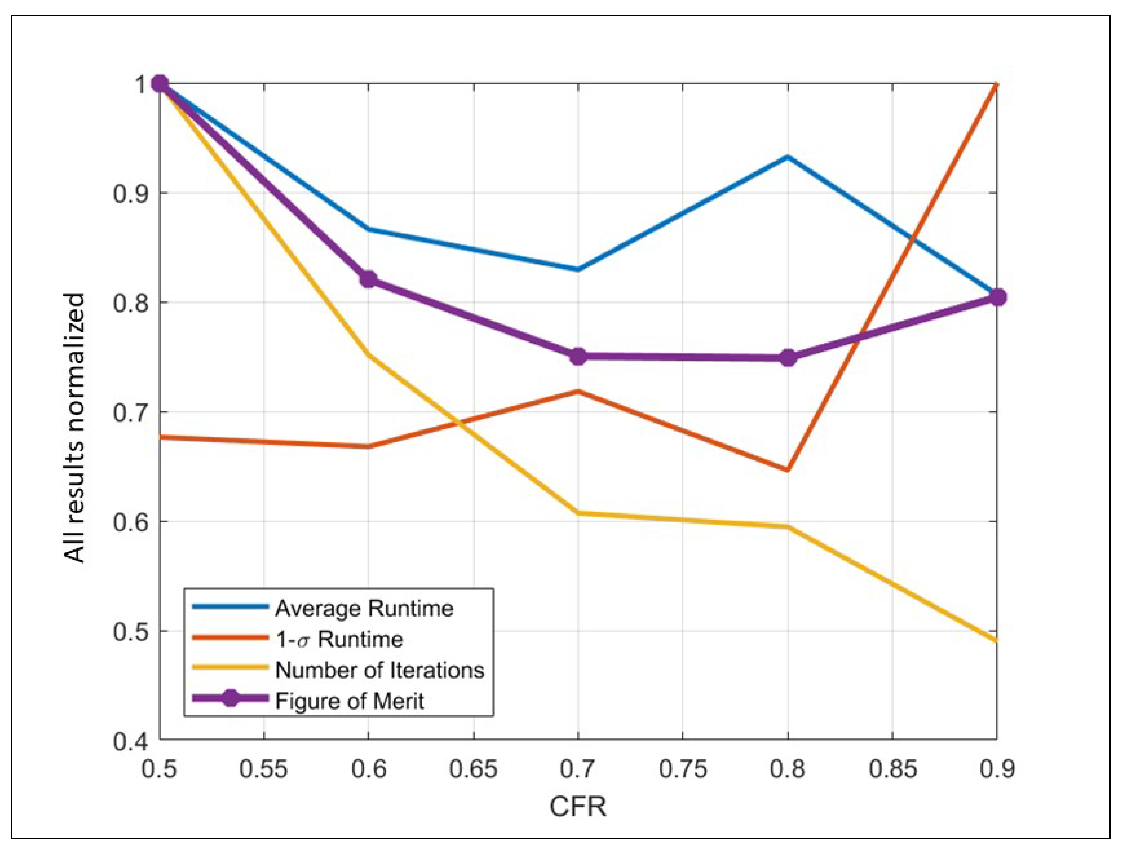
5. The Characteristic Frequency Ratio

We defined $f_{SURF}^c$ for a surface error map and calibrated $f_{TIF}^c$ for a TIF, and we illustrated the method of determining the size of a TIF using $f_{TIF}^c$. Now, we need a new criterion that can combine $f_{SURF}^c$ with $f_{TIF}^c$ to guide tool size selection based on a particular surface error map. To accomplish this, we define the characteristic frequency ratio (CFR), which is simply the ratio between the CF of a TIF and the CF of a surface error map such that

$$\mathrm{CFR}=\frac{f_{TIF}^c}{f_{SURF}^c}.$$

(12)

This simple ratio allows us to quantitatively set the TIF size based on the spatial frequency distribution of the surface error. A CFR of one, based on the definition given in Section 2.4, theoretically implies that the given TIF will correct 80% of the surface error. However, this setting may cost too much processing time, negatively influencing the processing efficiency. In addition, because this TIF only corrects the lower 80% frequency modes, the remaining 20% of the error is now due to higher spatial frequencies not suited for the initial TIF, and thus a new, smaller TIF is now required. Although the frequency content of the new residual error map has changed, the CFR should be able to be used once again to set this TIF size appropriately. Therefore, a well-selected CFR for each TIF is critical for the overall accuracy and efficiency of the fabrication process.

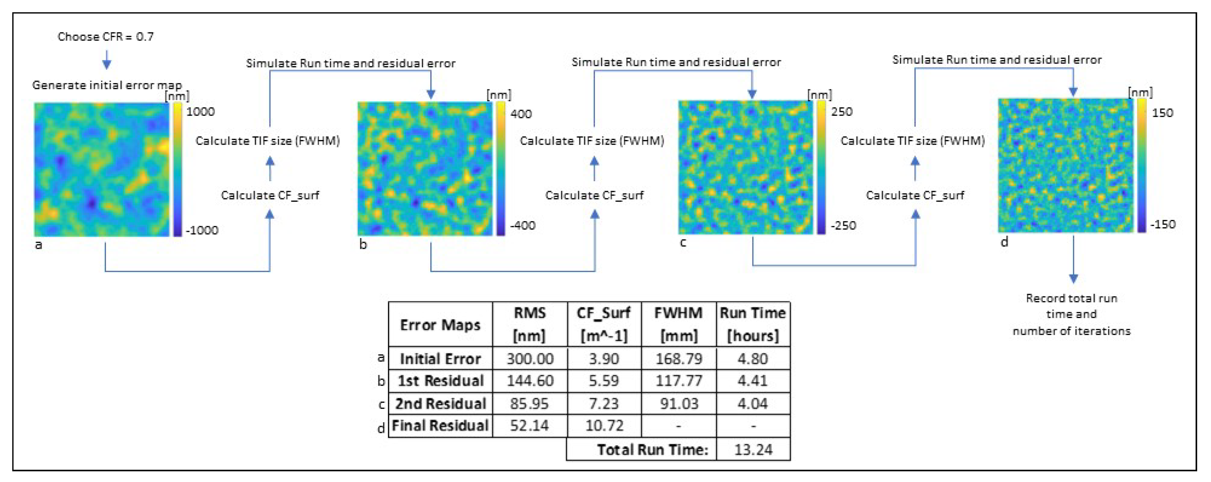
6. Computer-Assisted Study of the Optimal CFR for Tool Size Selection

An optimal CFR should consider the following aspects. First, it should balance the accuracy and efficiency. In other words, we expect that the target residual RMS error can be achieved in the shortest available total run time of all the tools. Secondly, the number of iterations (i.e., the number of tools employed to achieve the target) should be as small as possible, since frequent changing of tools also influences the overall efficiency. Finally, the selected CFR should be stable so that the same CFR can be applied to select the tool size in each iteration. Based on these philosophies, a computer simulation was designed and conducted to statistically study the optimal CFR.

6.1. Simulation Specifications

To study the optimal CFR, different CFR values were applied to select tool sizes for many initial surface error maps that were randomly generated with the same RMS value.

In detail, similar to the surface error map shown in Figure 3a, for a single test case, we first generated a random surface error map with a size of 1.85 m × 1.85 m by using the measured PSD trend of the aspheric DKIST primary mirror [24], adding random amounts of low-to-medium spatial frequency errors and scaling to the same total RMS.

Next, a CFR value was selected to investigate, with $\mathrm{CFR}\in \{0.5,0.6,0.7,0.8,0.9\}$. The CFR, along with the CF of the given surface error map, was used to define the TIF size as detailed in Section 4. The robust iterative Fourier transform-based dwell time algorithm (RIFTA) [25] was used to determine the residual error and the total run time for each iteration, since the RIFTA is fast and minimizes the residual and run time simultaneously. Afterward, on the residual error map, another TIF was chosen with the same method. This procedure was repeated for this test case until the surface was within the target RMS bounds, which were set to be 15% ± 3% of the initial RMS. Each test case (i.e., a certain CFR value) was run on 30 separate randomly generated surface error maps, and the average total run time, run time standard deviation, and average number of iterations over the 30 trials were recorded.

Figure 6 depicts one set of this process on a single initial surface error map. The selected CFR was 0.7, and dwell time optimization with the RIFTA was performed on the residual surface errors iteratively until the target RMS was reached.

6.2. Simulation Results

The results of the simulation are shown in Figure 7. To compare the results of each case, we defined a figure of merit (FoM) for one case to be the root sum square (RSS) of the average run time, standard deviation of the run time, and average number of iterations, each normalized by the maximum case value for its respective category. A smaller FoM value thus corresponds to a more efficient CFR. As shown in Figure 7, the small FoM values appeared between $\mathrm{CFR}=0.7$ and $\mathrm{CFR}=0.8$.

The average run time of each case is shown by in the blue line in Figure 7, which was calculated as the mean run time of the 30 runs of the same CFR. It is obvious that $\mathrm{CFR}=0.5$ and $\mathrm{CFR}=0.8$ do not appear to be a good choice because of their longer run times. The standard deviation of the total run time of each case is shown in red in Figure 7, which represents the stability of the selected CFR. It was found that $\mathrm{CFR}=0.9$ was not very stable. Finally, the average number of iterations of each case that was spent to achieve the target residual error is given in yellow in Figure 7. A small number of iterations indicates a higher overall efficiency for the selected CFR value, primarily due to the down time caused by tool changes. Therefore, larger CFR values tend to be more efficient under this definition than smaller CFR values. It is clear by interpolation that the consistent use of a CFR within 0.75 yielded the most stable balance among the accuracy, total run time, and number of required iterations. Thus, it was selected as a general criterion in choosing tool sizes in CCOS.

7. Conclusions

In this paper, we proposed a straightforward characteristic frequency ratio (CFR) to guide tool size selection in computer-controlled optical surfacing (CCOS) processes. The proposed CFR was statistically studied via computer simulation, and it was the first general criterion that considered both the residual errors and total run time.

The CFR is defined as the ratio between the characteristic frequencies (CFs) of a surface error map and a tool influence function (TIF). While the CF of a surface error map is defined according to the proposed encircled error metric, the CF of a TIF is calibrated based on a reference surface error map containing a single sinusoidal frequency and a reference TIF derived from Preston’s equation. Based on the novel integrated PSD of a TIF metric, the method for generalizing the calibrated CF to determine the sizes of different kinds of TIFs in typical CCOS processes was then presented, verifying the applicability of the method. Finally, the proposed idea was statistically studied with a well-designed computer simulation on many initial surface error maps and different CFRs. The simulation results demonstrate that a CFR of 0.75 consistently achieves the most stable balance among the residual error, total run time, and total number of iterations and thus can be chosen as a simple criterion to guide tool size selection.

References

1. Jones, R.A. Optimization of computer controlled polishing. Appl. Opt. 1977, 16, 218–224. [Google Scholar] [CrossRef]
2. Cheng, H. Independent Variables for Optical Surfacing Systems; Springer: Berlin/Heidelberg, Germany, 2016. [Google Scholar]
3. Fanson, J.; Bernstein, R.; Angeli, G.; Ashby, D.; Bigelow, B.; Brossus, G.; Bouchez, A.; Burgett, W.; Contos, A.; Demers, R.; et al. Overview and status of the Giant Magellan Telescope project. In Proceedings of the Ground-based and Airborne Telescopes VIII. International Society for Optics and Photonics, Online, 14–22 December 2020; Volume 11445, p. 114451F. [Google Scholar]
4. Ghigo, M.; Vecchi, G.; Basso, S.; Citterio, O.; Civitani, M.; Mattaini, E.; Pareschi, G.; Sironi, G. Ion figuring of large prototype mirror segments for the E-ELT. Adv. Opt. Mech. Technol. Telesc. Instrum. 2014, 9151, 225–236. [Google Scholar]
5. Kim, D.; Choi, H.; Brendel, T.; Quach, H.; Esparza, M.; Kang, H.; Feng, Y.T.; Ashcraft, J.N.; Ke, X.; Wang, T.; et al. Advances in Optical Engineering for Future Telescopes. Opto-Electron. Adv. 2021, 4, 210040-1. [Google Scholar] [CrossRef]
6. Schindler, A.; Haensel, T.; Nickel, A.; Thomas, H.J.; Lammert, H.; Siewert, F. Finishing procedure for high-performance synchrotron optics. Opt. Manuf. Test. V 2003, 5180, 64–72. [Google Scholar]
7. Beaucamp, A.; Namba, Y. Super-smooth finishing of diamond turned hard X-ray molding dies by combined fluid jet and bonnet polishing. CIRP Ann. 2013, 62, 315–318. [Google Scholar] [CrossRef]
8. Thiess, H.; Lasser, H.; Siewert, F. Fabrication of X-ray mirrors for synchrotron applications. Nucl. Instrum. Methods Phys. Res. Sect. A Accel. Spectrometers Detect. Assoc. Equip. 2010, 616, 157–161. [Google Scholar] [CrossRef]
9. Wang, T.; Huang, L.; Choi, H.; Vescovi, M.; Kuhne, D.; Zhu, Y.; Pullen, W.C.; Ke, X.; Kim, D.W.; Kemao, Q.; et al. RISE: Robust iterative surface extension for sub-nanometer X-ray mirror fabrication. Opt. Express 2021, 29, 15114–15132. [Google Scholar] [CrossRef]
10. Wang, T.; Huang, L.; Vescovi, M.; Kuhne, D.; Zhu, Y.; Negi, V.S.; Zhang, Z.; Wang, C.; Ke, X.; Choi, H.; et al. Universal dwell time optimization for deterministic optics fabrication. Opt. Express 2021, 29, 38737–38757. [Google Scholar] [CrossRef]
11. Weiser, M. Ion beam figuring for lithography optics. Nucl. Instrum. Methods Phys. Res. Sect. B Beam Interact. Mater. Atoms. 2009, 267, 1390–1393. [Google Scholar] [CrossRef]
12. Wischmeier, L.; Graeupner, P.; Kuerz, P.; Kaiser, W.; van Schoot, J.; Mallmann, J.; de Pee, J.; Stoeldraijer, J. High-NA EUV lithography optics becomes reality. Extrem. Ultrav. (EUV) Lithogr. XI 2020, 11323, 1132308. [Google Scholar]
13. Han, Y.; Duan, F.; Zhu, W.; Zhang, L.; Beaucamp, A. Analytical and stochastic modeling of surface topography in time-dependent sub-aperture processing. Int. J. Mech. Sci. 2020, 175, 105575. [Google Scholar] [CrossRef]
14. Chaves-Jacob, J.; Beaucamp, A.; Zhu, W.; Kono, D.; Linares, J.M. Towards an understanding of surface finishing with compliant tools using a fast and accurate simulation method. Int. J. Mach. Tools Manuf. 2021, 163, 103704. [Google Scholar] [CrossRef]
15. Zhou, L.; Dai, Y.; Xie, X.; Li, S. Frequency-domain analysis of computer-controlled optical surfacing processes. Sci. China Ser. E Technol. Sci. 2009, 52, 2061–2068. [Google Scholar] [CrossRef]
16. Wang, J.; Fan, B.; Wan, Y.; Shi, C.; Zhuo, B. Method to calculate the error correction ability of tool influence function in certain polishing conditions. Opt. Eng. 2014, 53, 075106. [Google Scholar] [CrossRef]
17. Wang, J.; Hou, X.; Wan, Y.; Shi, C. An optimized method to calculate error correction capability of tool influence function in frequency domain. Optifab 2017 2017, 10448, 104481Z. [Google Scholar]
18. Trumper, I.; Hallibert, P.; Arenberg, J.W.; Kunieda, H.; Guyon, O.; Stahl, H.P.; Kim, D.W. Optics technology for large-aperture space telescopes: From fabrication to final acceptance tests. Adv. Opt. Photonics 2018, 10, 644–702. [Google Scholar] [CrossRef]
19. Graves, L.R.; Smith, G.A.; Apai, D.; Kim, D.W. Precision Optics Manufacturing and Control for Next-Generation Large Telescopes. J. Int. Soc. Nanomanuf. 2019, 2, 65–90. [Google Scholar] [CrossRef]
20. Jacobs, T.D.; Junge, T.; Pastewka, L. Quantitative characterization of surface topography using spectral analysis. Surf. Topogr. Metrol. Prop. 2017, 5, 013001. [Google Scholar] [CrossRef] [Green Version]
21. Kim, D.W.; Kim, S.W.; Burge, J.H. Non-sequential optimization technique for a computer controlled optical surfacing process using multiple tool influence functions. Opt. Express 2009, 17, 21850–21866. [Google Scholar] [CrossRef] [Green Version]
22. Kim, D.W.; Park, W.H.; Kim, S.W.; Burge, J.H. Parametric modeling of edge effects for polishing tool influence functions. Opt. Express 2009, 17, 5656–5665. [Google Scholar]
23. Dong, Z.; Cheng, H.; Tam, H.Y. Modified subaperture tool influence functions of a flat-pitch polisher with reverse-calculated material removal rate. Appl. Opt. 2014, 53, 2455–2464. [Google Scholar] [CrossRef] [PubMed]
24. Kim, D.W.; Oh, C.J.; Lowman, A.; Smith, G.A.; Aftab, M.; Burge, J.H. Manufacturing of super-polished large aspheric/freeform optics. Adv. Opt. Mech. Technol. Telesc. Instrum. II 2016, 9912, 99120F. [Google Scholar]
25. Wang, T.; Huang, L.; Kang, H.; Choi, H.; Kim, D.W.; Tayabaly, K.; Idir, M. RIFTA: A Robust Iterative Fourier Transform-based dwell time Algorithm for ultra-precision ion beam figuring of synchrotron mirrors. Sci. Rep. 2020, 10, 8135. [Google Scholar] [CrossRef] [PubMed]
Figure 1. Schematic of the relationship between relevant surface parameters, where “★” is the auto-correlation operator, F and F 1 represent the forward and inverse Fourier transforms, respectively, and σ 2 is the variance of the surface profile.
Photonics 10 00286 g001
Figure 2. An example surface error map (a) and its 2D PSD map (b). The EE of the PSD (c) demonstrates that 80% of the RMS error was due to spatial frequencies lower than 3.41 m 1 .
Photonics 10 00286 g002
Figure 3. (a) The reference surface error map and (b) its 1D profile along the x direction.
Photonics 10 00286 g003
Figure 4. (a) Reference Line TIF with characteristic frequency f T I F c = 0.05 mm 1 , (b) 1D PSD of the reference Line TIF, and (c) IP of the reference TIF.
Photonics 10 00286 g004
Figure 5. Typical TIFs scaled to have a characteristic frequency of f c = 0.05 mm 1 .
Photonics 10 00286 g005
Figure 6. Simulation example for one iteration of test case with CFR = 0.7 showing (a) initial error map, (b) first residual error map, (c) second residual error map, and (d) final residual error map, with a table keeping track of the RMS value and CF of each map, the FWHM of the Gaussian TIF used on each map, and the calculated run time required for each run.
Photonics 10 00286 g006
Figure 7. Simulation results for the average total run time (blue), the standard deviation of the total run time (red), the average number of iterations (yellow), and the figure of merit (purple).
Photonics 10 00286 g007
Disclaimer/Publisher’s Note: The statements, opinions and data contained in all publications are solely those of the individual author(s) and contributor(s) and not of MDPI and/or the editor(s). MDPI and/or the editor(s) disclaim responsibility for any injury to people or property resulting from any ideas, methods, instructions or products referred to in the content.