Three-Dimensional Mapping Technology for Structural Deformation during Aircraft Assembly Process


Abstract
:1. Introduction
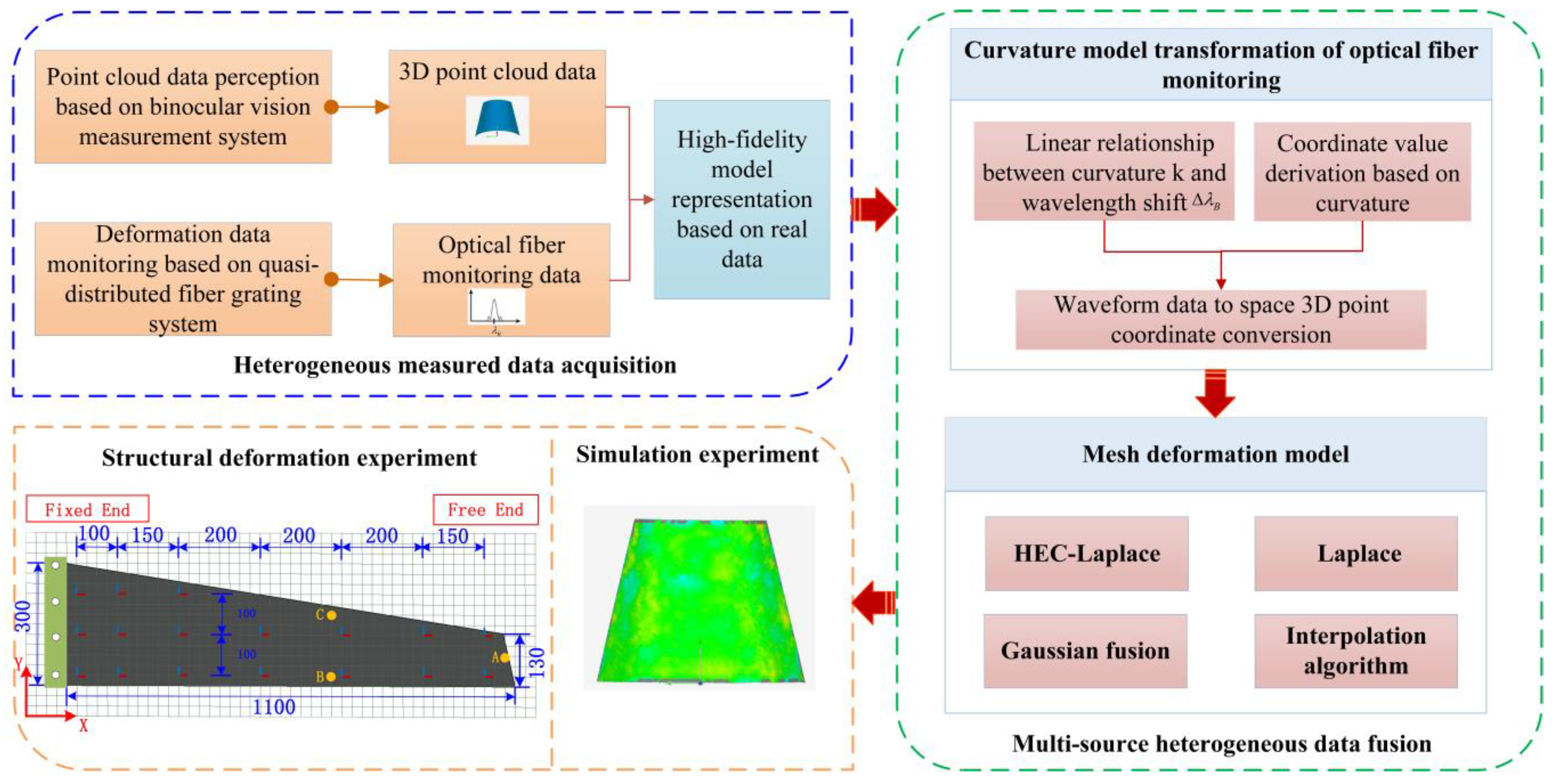
2. General Scheme
3. Methods
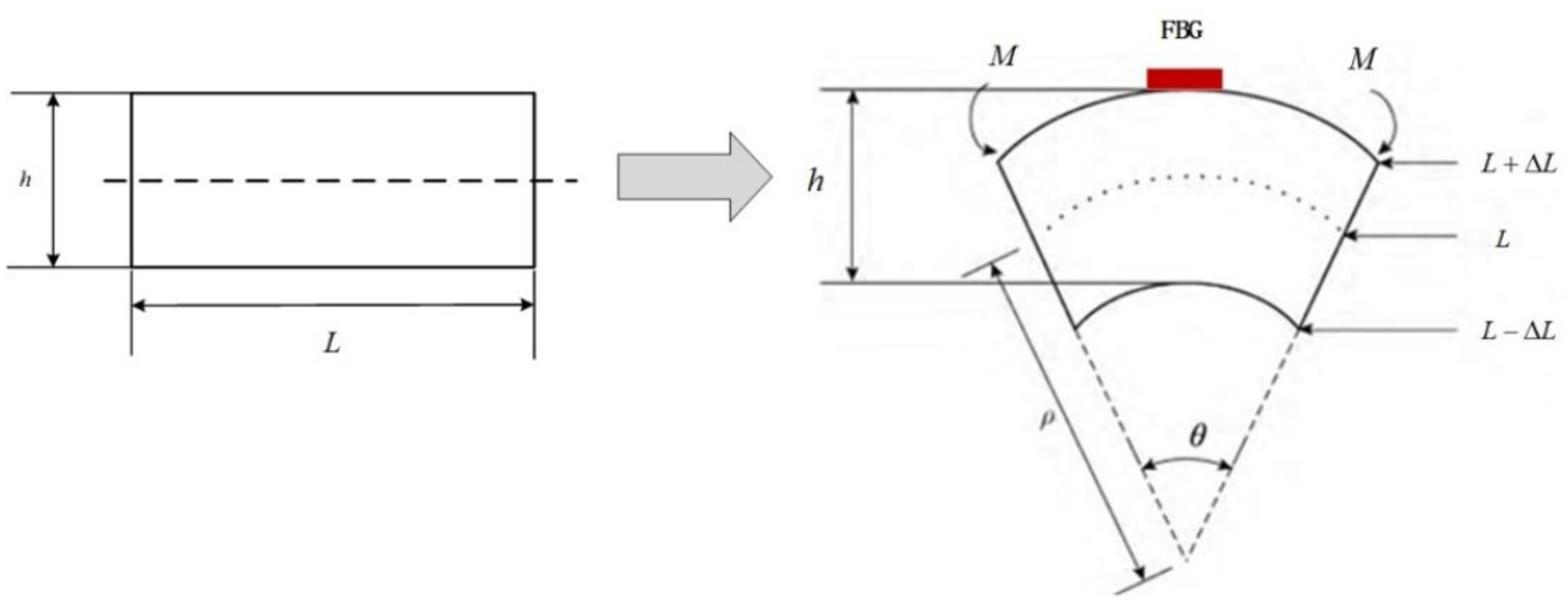
3.1. Curvature Conversion Model of Optical Fiber Monitoring
3.1.1. Curvature Conversion Model
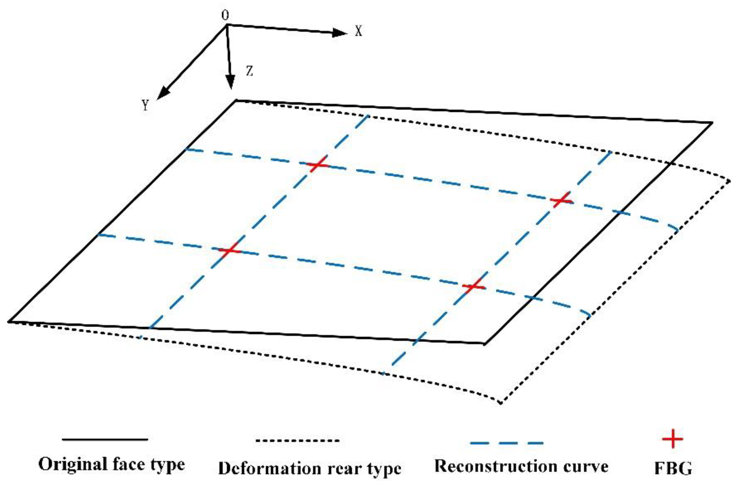
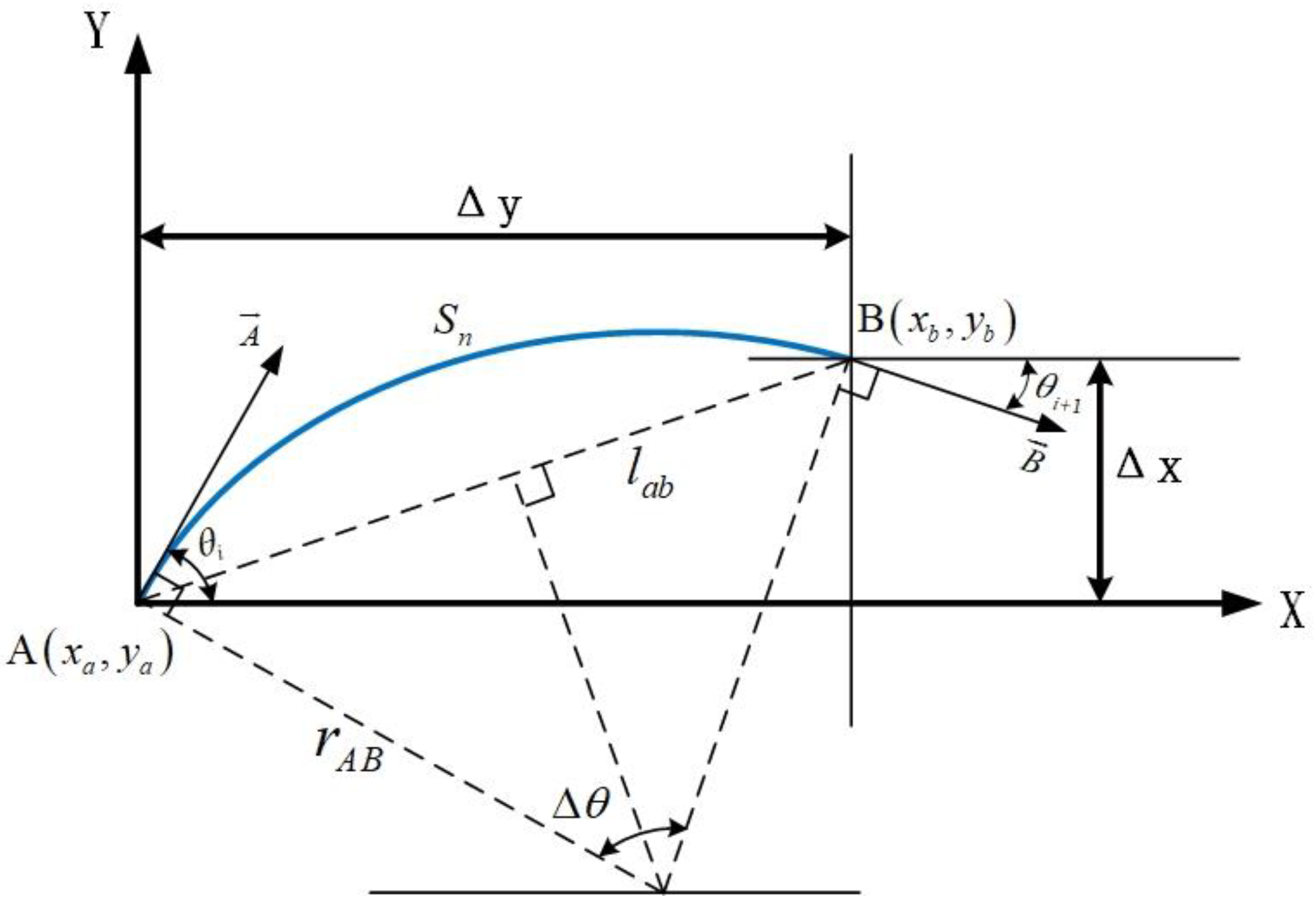
3.1.2. Coordinate Value Derivation Based on Curvature
3.2. Grid Distortion Optimization Algorithm for Base Point-Cloud Optimization
- Based on the optimized half-edge folding method, the original mesh model was simplified to obtain an optimized mesh with sparse point clouds but no effect on surface quality.
- The absolute coordinates of the mesh model were converted into differential coordinates.
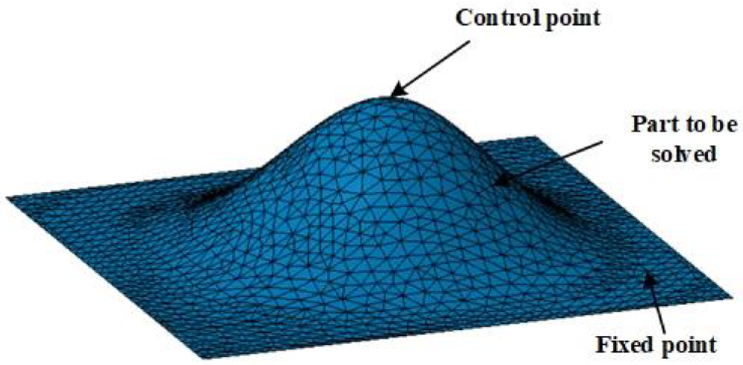
- The optical fiber monitoring point was set as the control point, and the mapping relationship between the original model and the control point was established.
- The absolute coordinate values of control points after distortion were obtained according to optical fiber monitoring data.
- The absolute coordinates of the other vertices of the distorted model were inverted based on the known differential coordinates and the absolute coordinates of the control points.
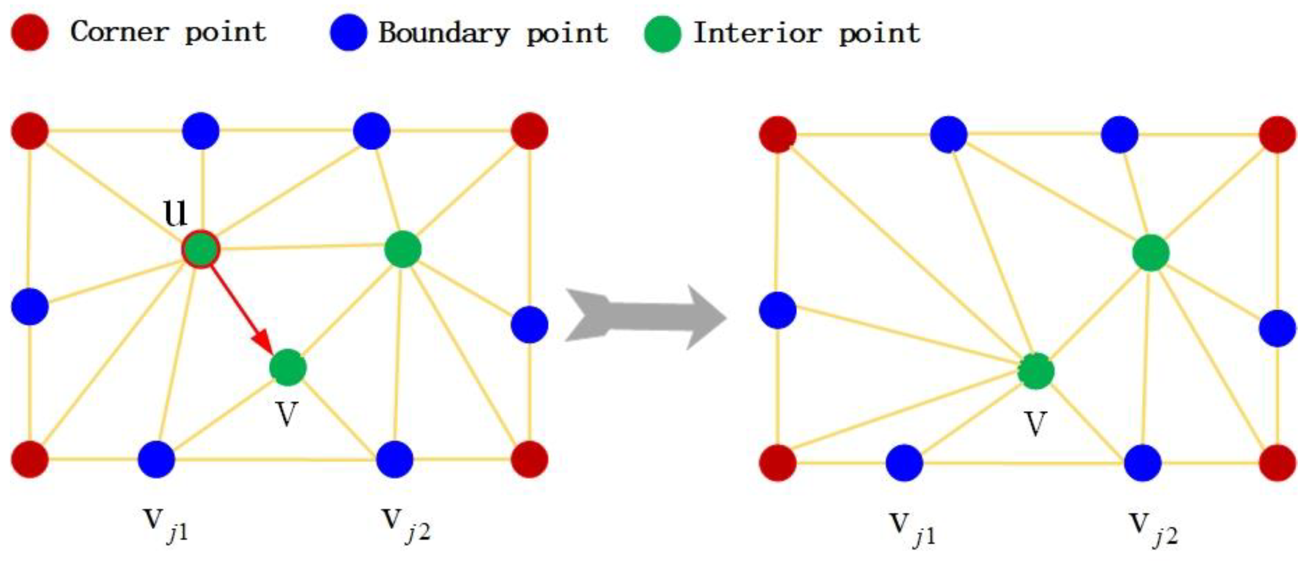
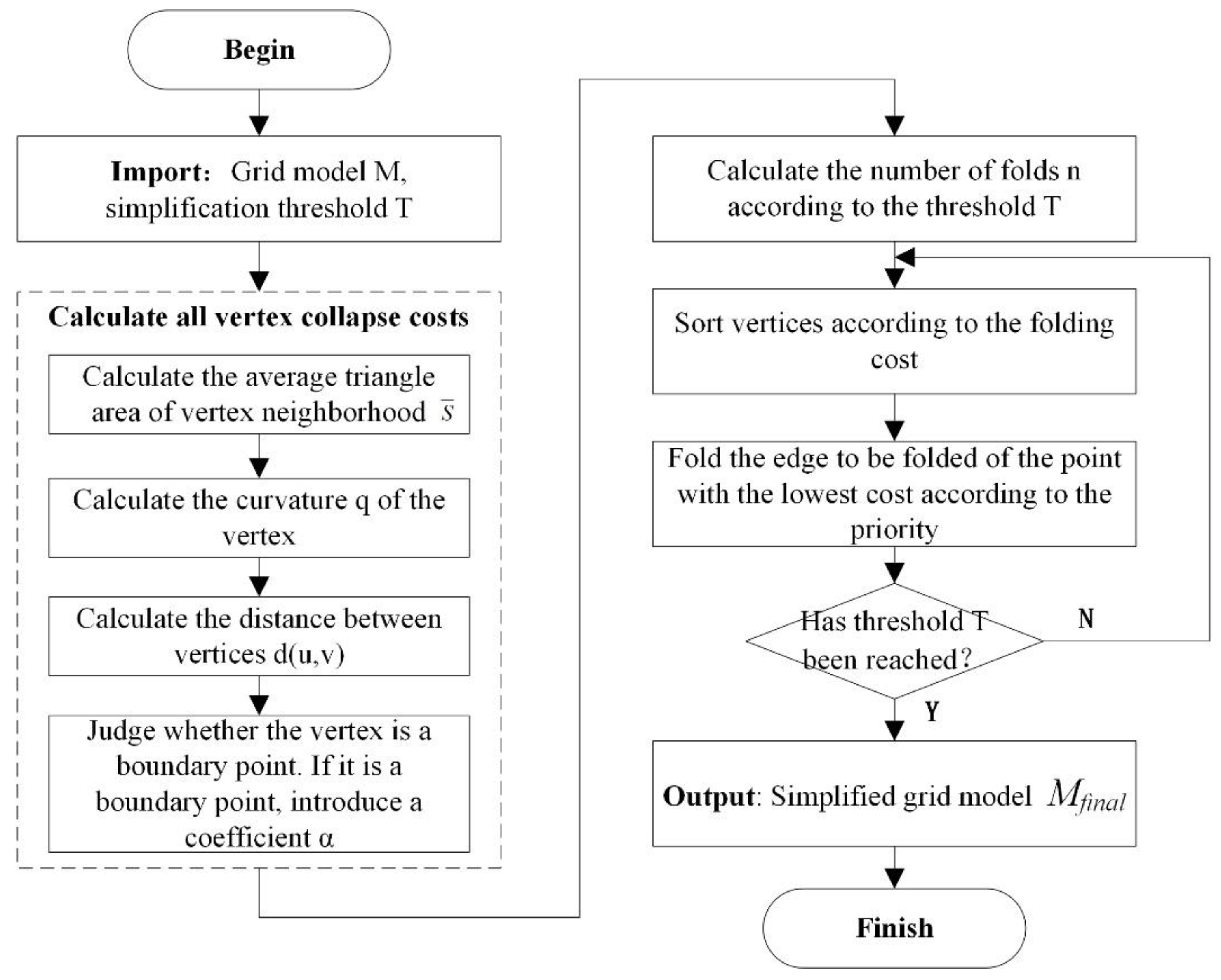
3.2.1. Model Simplification
- Calculation of the average area of a vertex neighborhood triangle
- 2.
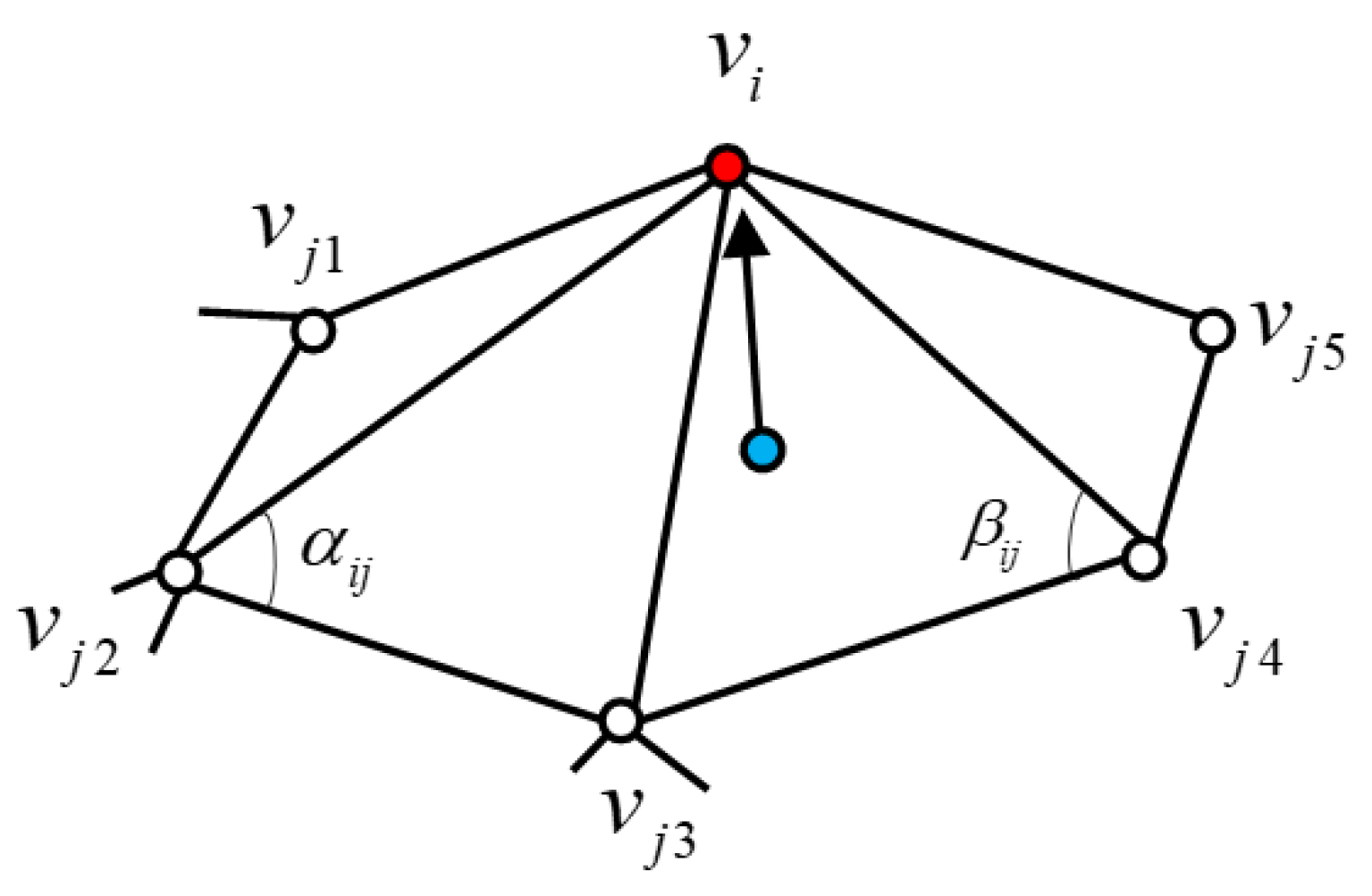
- Calculation of the discrete curvature of vertices
- 3.
- Determination of a boundary point
- 4.
- Calculation of distance between vertices
- 5.
- Fold cost calculation
3.2.2. Mesh Distortion Optimization Algorithm
- Laplacian mesh distortion
- 2.
- Laplacian matrix
- 3.
- Addition of constraints
- 4.
- Establishment of deformation constraints
3.2.3. Pseudocode
| Algorithm 1. Pseudocode for HEC-Laplace | |
| 1: | Input: Original grid control points before and after deformation simplification threshold |
| 2: | Output: Deformed grid runtime |
| 3: | Initialization: |
| 4: | Compute folding times based on simplification threshold |
| 5: | Model simplification: (Section 3.2.1) |
| 6: | Compute folding cost by Equation (15); |
| 7: | Sort vertices according to collapse cost; |
| 8: | Folding edges with the least cost by priority; |
| 9: | Grid Deformation: (Section 3.2.2) |
| 10: | Verify the set of one-ring neighborhood points for each vertex; |
| 11: | According to Equation (16) define the Laplace coordinates of the vertices; |
| 12: | According to Equation (17) compute cotangent weights; |
| 13: | Introduce a Laplacian matrix based on Equation (19) convert Cartesian coordinates to differential coordinates; |
| 14: | According to Equation (23) establishment of statically indeterminate systems of linear equations; |
| 15: | Solve equations to obtain the new position of the vertex under the Cartesian coordinate system. |
4. Results and Discussion
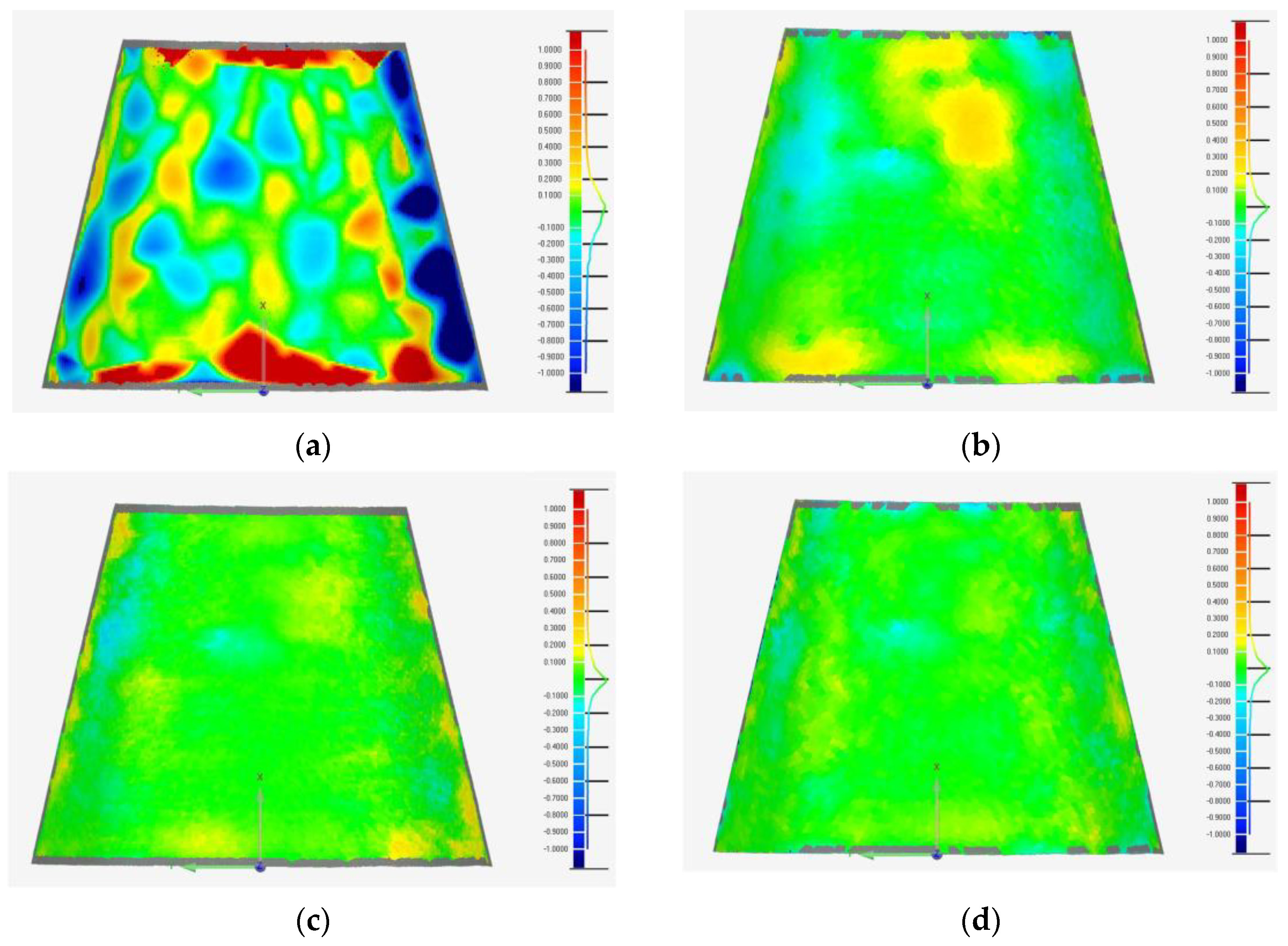
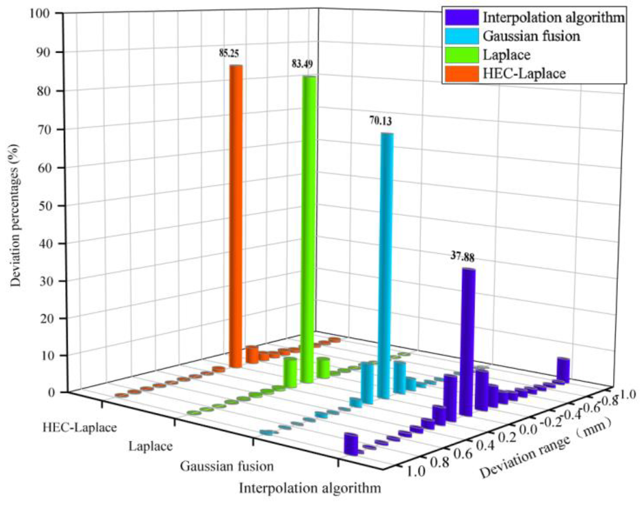
4.1. Comparison of Deformation Algorithm through Simulations
4.1.1. Model Evaluation
4.1.2. Simulation Experiments
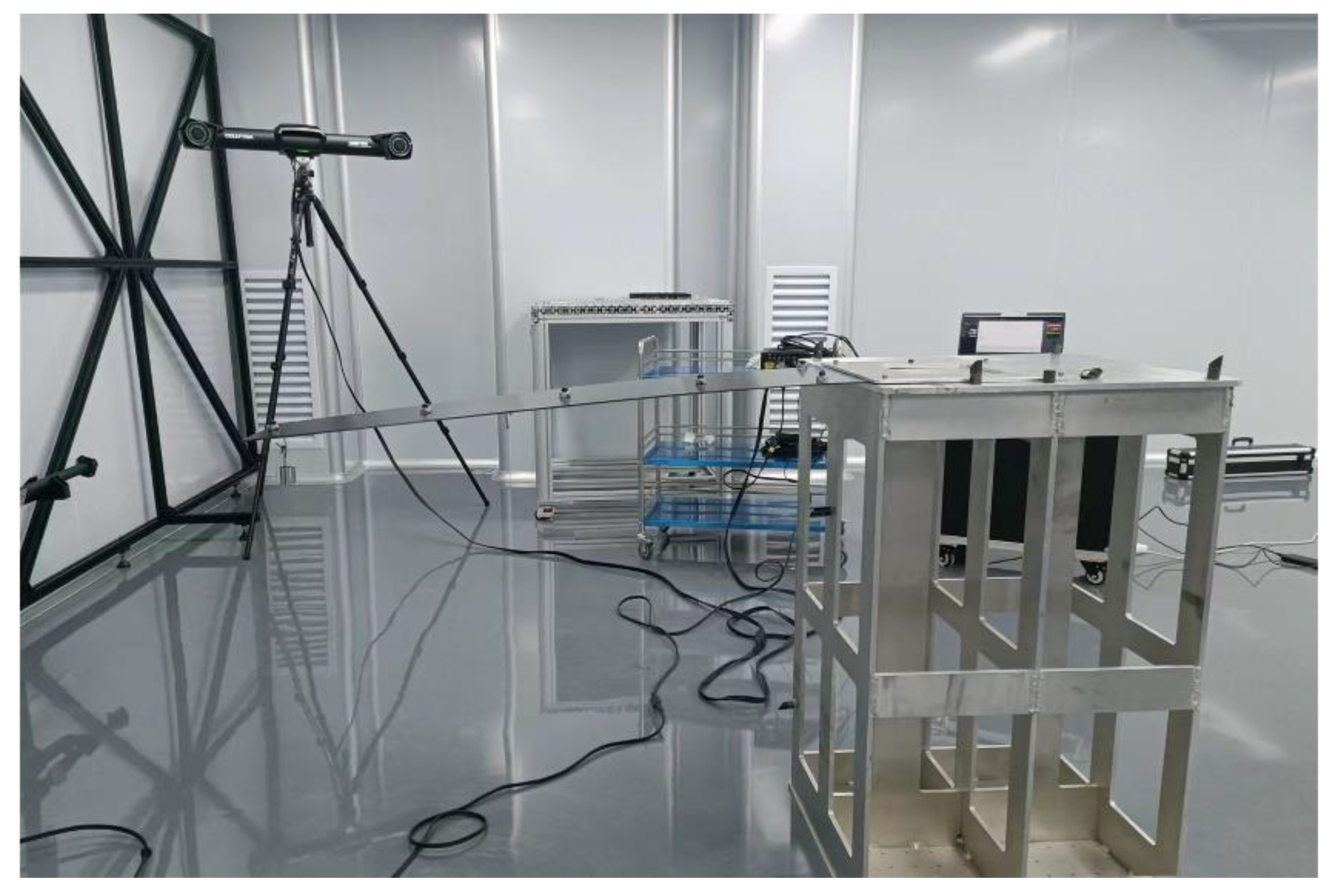
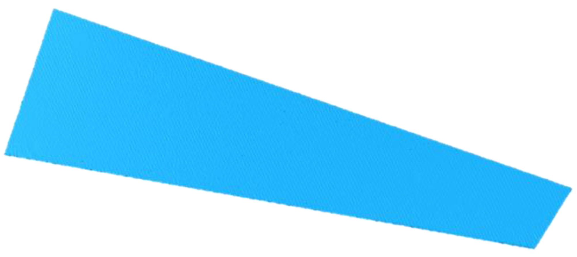
4.2. Application of Structural Deformation Mapping
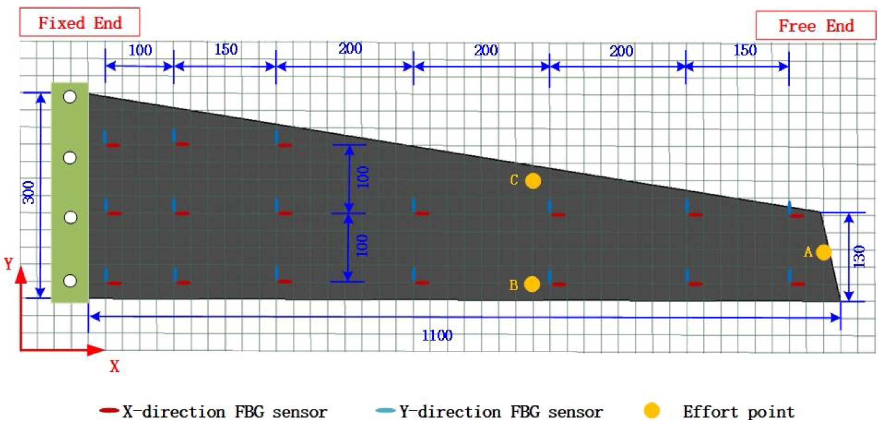
4.2.1. Establishment of Experimental System
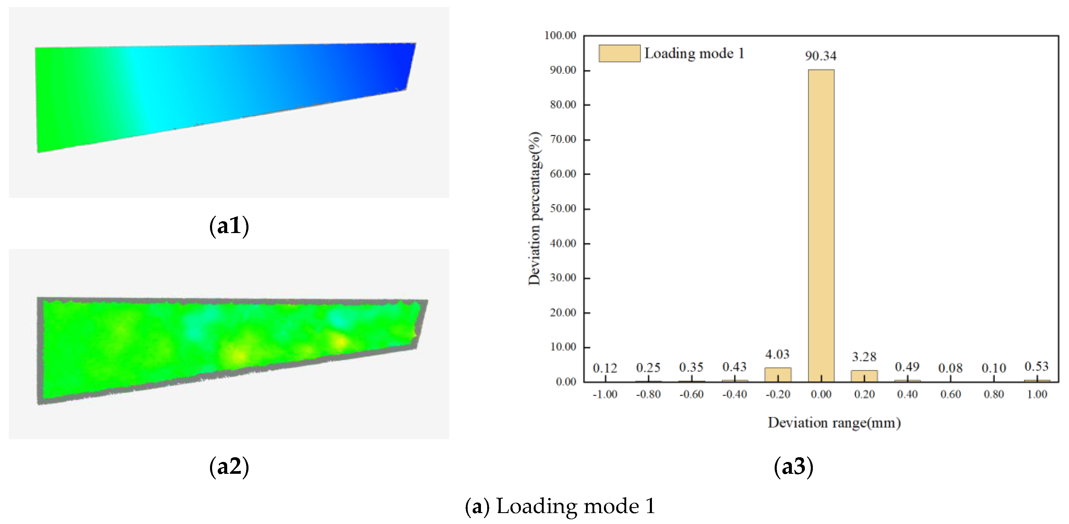
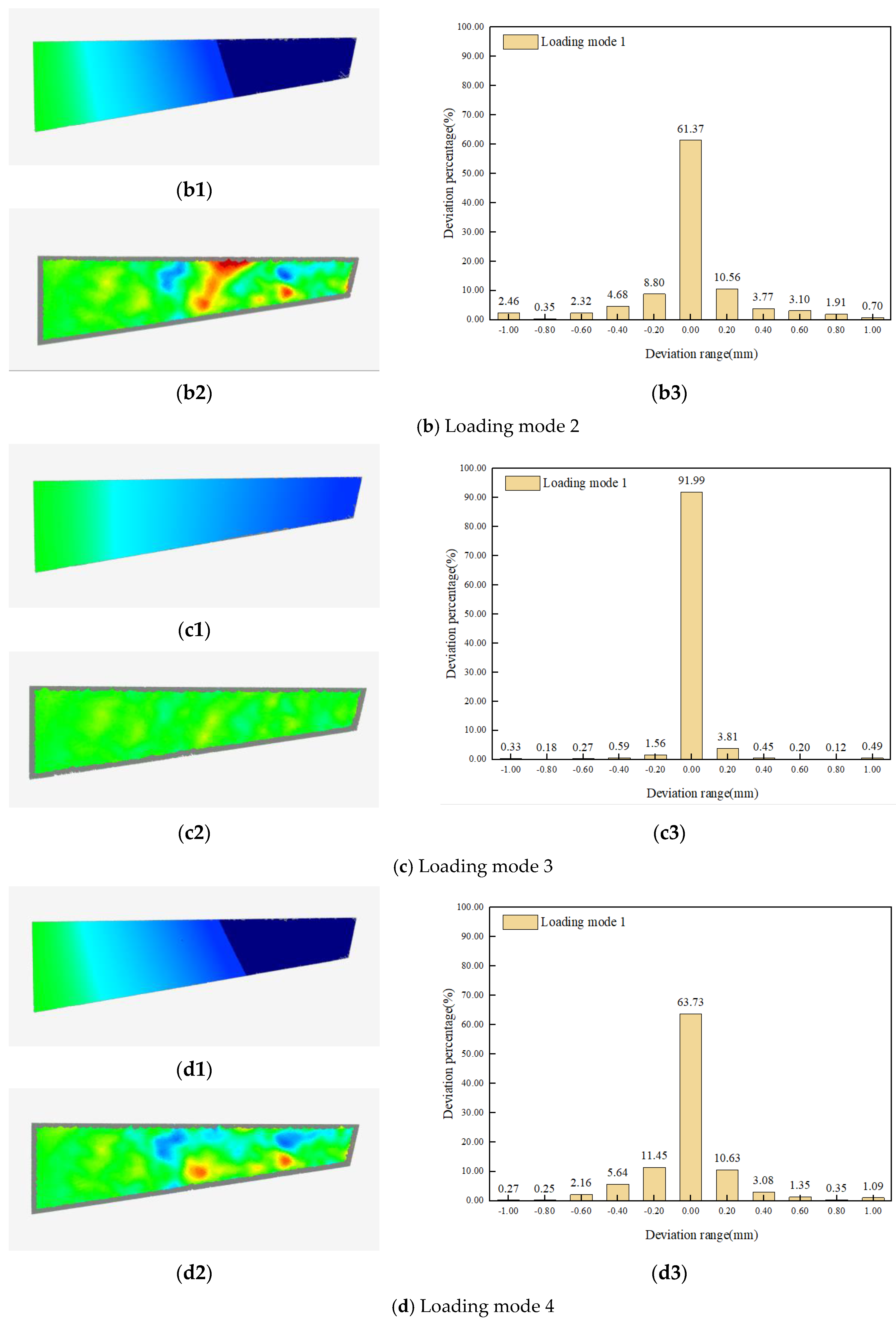
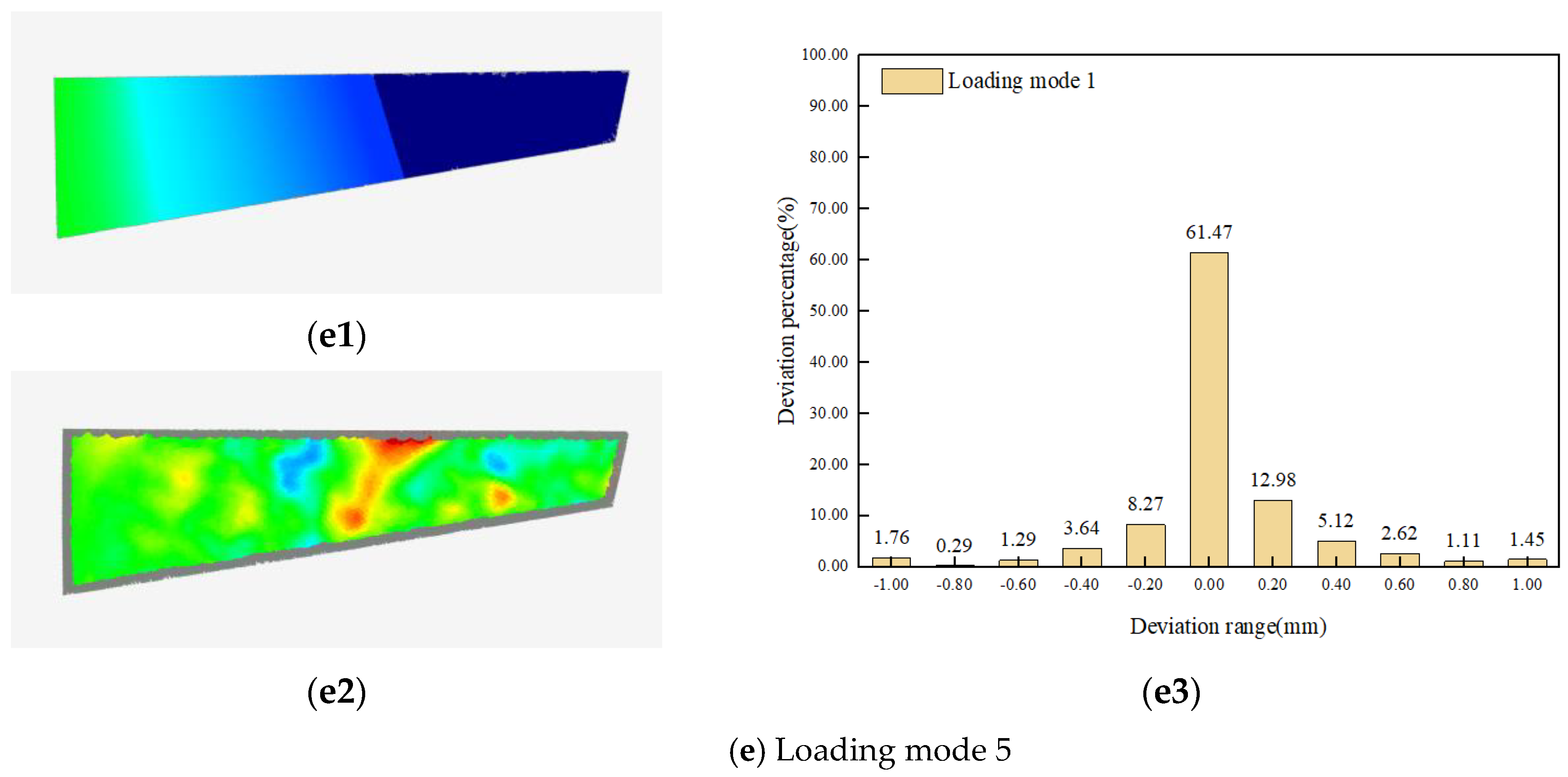
4.2.2. Experimental Results
5. Conclusions
Author Contributions
Funding
Institutional Review Board Statement
Informed Consent Statement
Data Availability Statement
Conflicts of Interest
References
- Zhao, Z.; Gan, X.; Liqun, M.A. A Combined Adjustment Network Method Based on Multi-Sensor System Cooperative Measurement. Chin. J. Sens. Actuators 2019, 32, 100–105. [Google Scholar]
- Zhang, Y.; Shen, Y.; Zhang, W.; Zhang, L.; Zhu, L.; Zhang, Y. Generation of efficient and interference-free scanning path for inspecting impeller on a cylindrical CMM. Measurement 2022, 198, 111352. [Google Scholar] [CrossRef]
- Chen, Z.; Zhang, F.; Qu, X.; Liang, B. Fast Measurement and Reconstruction of Large Workpieces with Freeform Surfaces by Combining Local Scanning and Global Position Data. Sensors 2015, 15, 14328–14344. [Google Scholar] [CrossRef] [PubMed] [Green Version]
- Ser’Eznov, A.N.; Stepanova, L.N.; Laznenko, A.S.; Kabanov, S.I.; Kozhemyakin, V.L.; Chernova, V.V. Static Tests of Wing Box of Composite Aircraft Wing Using Acoustic Emission and Strain Gaging. Russ. J. Nondestruct. Test. 2020, 56, 611–619. [Google Scholar] [CrossRef]
- Wang, Q.; Dou, Y.; Li, J.; Ke, Y.; Keogh, P.; Maropoulos, P.G. An assembly gap control method based on posture alignment of wing panels in aircraft assembly. Assem. Autom. 2017, 37, 422–433. [Google Scholar] [CrossRef] [Green Version]
- Zhang, W. Research on Digital Preassembly Technology of Aircraft Parts Based on Measured Data; Nanjing University of Aeronautics and Astronautics: Nanjing, China, 2016. [Google Scholar]
- Guo, F.; Liu, J.; Zou, F.; Zhai, Y.; Wang, Z.; Li, S. Research on assembly process design and key implementation technology of digital twin drive. Chin. J. Mech. Eng. 2019, 55, 110–132. [Google Scholar]
- Sun, G.; Wu, Y.; Li, H.; Zhu, L. 3D shape sensing of flexible morphing wing using fiber Bragg grating sensing method. Optik 2018, 156, 83–92. [Google Scholar] [CrossRef]
- Ma, Z.; Chen, X. Strain transfer characteristics of surface-attached FBGs in aircraft wing distributed deformation measurement. Optik 2020, 207, 164468. [Google Scholar] [CrossRef]
- Wang, B.; Fan, S.; Chen, Y.; Zheng, L.; Zhu, H.; Fang, Z.; Zhang, M. The replacement of dysfunctional sensors based on the digital twin method during the cutter suction dredger construction process measurement. Measurement 2022, 189, 110523. [Google Scholar] [CrossRef]
- Zhang, S.; Yan, J.; Jiang, M.; Sui, Q.; Zhang, L.; Luo, Y. Visual reconstruction of flexible structure based on fiber grating sensor array and extreme learning machine algorithm. Optoelectron. Lett. 2022, 18, 390–397. [Google Scholar] [CrossRef]
- Brindisi, A.; Vendittozzi, C.; Travascio, L.; Di Palma, L.; Ignarra, M.; Fiorillo, V.; Concilio, A. A Preliminary Assessment of an FBG-Based Hard Landing Monitoring System. Photonics 2021, 8, 450. [Google Scholar] [CrossRef]
- Ding, G.; Wang, F.; Gao, X.; Jiang, S. Research on Deformation Reconstruction Based on Structural Curvature of CFRP Propeller with Fiber Bragg Grating Sensor Network. Photon- Sens. 2022, 12, 220412. [Google Scholar] [CrossRef]
- Yi, L.; Xue, Z.; Ding, Y.; Wang, M.; Guo, Z.; Shi, J. Surface Curvature Sensor Based on Intracavity Sensing of Fiber Ring Laser. Photonics 2022, 9, 781. [Google Scholar] [CrossRef]
- Alexa, M. Differential coordinates for local mesh morphing and deformation. Vis. Comput. 2003, 19, 105–114. [Google Scholar] [CrossRef]
- Jäckle, S.; Strehlow, J.; Heldmann, S. Shape sensing with fiber bragg grating sensors-a realistic model of curvature interpolation for shape reconstruction. In Bildverarbeitung für die Medizin; Springer: Wiesbaden, Germany, 2019; pp. 258–263. [Google Scholar]
- Taubin, G. Estimating the tensor of curvature of a surface from a polyhedral approximation. In Proceedings of the IEEE International Conference on Computer Vision, Cambridge, MA, USA, 20–23 June 1995. [Google Scholar]
- Hao, J.; Tang, L.; Zeng, P. A Simplification Algorithm for Curvature and Area-Weighted Quadric Error Metrics Mesh. J. Donghua Univ. 2012, 38, 318–322. [Google Scholar]
- Ding, J.; Liu, T.-Y.; Bai, L.; Sun, Z. A multisensor data fusion method based on gaussian process model for precision measurement of complex surfaces. Sensors 2020, 20, 278. [Google Scholar] [CrossRef] [PubMed] [Green Version]
- González-Gaxiola, O.; Biswas, A.; Moraru, L.; Moldovanu, S. Highly Dispersive Optical Solitons in Absence of Self-Phase Modulation by Laplace-Adomian Decomposition. Photonics 2023, 10, 114. [Google Scholar] [CrossRef]
- Wu, J.; Cai, X.; Wei, J.; Wang, C.; Zhou, Y.; Sun, K. A Measurement System with High Precision and Large Range for Structured Surface Metrology Based on Atomic Force Microscope. Photonics 2023, 10, 289. [Google Scholar] [CrossRef]


| Model | Evaluation Index | |||
|---|---|---|---|---|
| MAE | RE | RMSE | Time (s) | |
| Interpolation algorithm | 0.388 | 19.77% | 0.609 | 10.47 |
| Gaussian fusion | 0.064 | 5.28% | 0.090 | 50.54 |
| Laplace | 0.058 | 3.47% | 0.075 | 591.22 |
| HEC−Laplace | 0.046 | 2.92% | 0.062 | 42.47 |
| Node Number | Loading Mode | Load Size | Load Application Position |
|---|---|---|---|
| 1 | Single point | 2 N | Point A |
| 2 | Single point | 5 N | Point A |
| 3 | Single point | 5 N | Point B |
| 4 | Multipoint loading | 2 N 5 N | Point A Point C |
| 5 | Multipoint loading | 2 × 5 N | Points B and C |
| Node Number | Maximum Deformation (mm) | Evaluation Index | ||
|---|---|---|---|---|
| MAE | RE | RMSE | ||
| 1 | 29.94 | 0.104 | 3.78% | 0.146 |
| 2 | 73.68 | 0.210 | 3.02% | 0.307 |
| 3 | 28.06 | 0.094 | 2.62% | 0.111 |
| 4 | 64.03 | 0.200 | 2.82% | 0.272 |
| 5 | 63.70 | 0.247 | 3.50% | 0.325 |
Disclaimer/Publisher’s Note: The statements, opinions and data contained in all publications are solely those of the individual author(s) and contributor(s) and not of MDPI and/or the editor(s). MDPI and/or the editor(s) disclaim responsibility for any injury to people or property resulting from any ideas, methods, instructions or products referred to in the content. |
© 2023 by the authors. Licensee MDPI, Basel, Switzerland. This article is an open access article distributed under the terms and conditions of the Creative Commons Attribution (CC BY) license (https://creativecommons.org/licenses/by/4.0/).
Share and Cite
Liu, Y.; Yan, D.; Li, L.; Lin, X.; Guo, L. Three-Dimensional Mapping Technology for Structural Deformation during Aircraft Assembly Process. Photonics 2023, 10, 318. https://doi.org/10.3390/photonics10030318
Liu Y, Yan D, Li L, Lin X, Guo L. Three-Dimensional Mapping Technology for Structural Deformation during Aircraft Assembly Process. Photonics. 2023; 10(3):318. https://doi.org/10.3390/photonics10030318
Chicago/Turabian StyleLiu, Yue, Dongming Yan, Lijuan Li, Xuezhu Lin, and Lili Guo. 2023. "Three-Dimensional Mapping Technology for Structural Deformation during Aircraft Assembly Process" Photonics 10, no. 3: 318. https://doi.org/10.3390/photonics10030318