Observer-Based State Estimation for Recurrent Neural Networks: An Output-Predicting and LPV-Based Approach

Abstract

An innovative cascade predictor is presented in this study to forecast the state of recurrent neural networks (RNNs) with delayed output. This cascade predictor is a chain-structured observer, as opposed to the conventional single observer, and is made up of several sub-observers that individually estimate the state of the neurons at various periods. This new cascade predictor is more useful than the conventional single observer in predicting neural network states when the output delay is arbitrarily large but known. In contrast to examining the stability of error systems solely employing the Lyapunov–Krasovskii functional (LKF), several new global asymptotic stability standards are obtained by combining the application of the Linear Parameter Varying (LPV) approach, LKF and convex principle. Finally, a series of numerical simulations verify the efficacy of the obtained results.

1. Introduction

Over the past decades, delayed recurrent neural networks were successfully applied in many fields, including pattern recognition, image processing, and combinatorial optimization [1,2,3,4,5], and the dynamic behaviors of RNNs have quickly become a research hotspot. At present, many stability results about the dynamic behavior of RNNs have been obtained [6,7,8,9,10,11,12]. Meanwhile, the state information of neurons is very important, because it may participate in the design process of control law, such as feedback control. Therefore, neural networks’ state estimation research is of significant importance in practical applications.

The issue of state estimation for RNNs is currently of great interest to many scholars, and many significant results have been made [13,14,15,16,17,18,19,20]. In [13], the authors discussed the state estimation problem for delayed RNNs and obtained delay-independent results using LMI technique. The state estimation problem for Markov jump RNNs with distributed delays was discussed in [14]; the authors proposed an effective LMI technique to solve the problem of neuron states’ estimation. The state estimation problem of uncertain RNNs was addressed via a robust state estimator in [15], and it was shown that the suggested robust estimator can be ensured by the feasibility of solving a set of LMIs. An interesting delay partition method was proposed in [17]; the authors used this method to investigate the state estimation problem for delayed static neural networks. In [20], the authors solved the memristive neural networks’ (MNNs) state estimation problem by using a novel full-order state observer. It is well known that the effectiveness of the designed observer is usually related to system parameters and the size of various time delays. For example, in most of the works mentioned above, the output states do not have a time delay or the size of the delay is limited to a small range, and a full-order observer is designed based on the measured output. In [21], during the identification of RNN models, a subspace encoder is co-estimated to reconstruct the state of the model from past input and output data. However, such an explicit form of an observer might run into difficulties if the state delay is not known, and needs an excessively large number of past input–output samples.

For arbitrary large known output delays, it is still an open problem to construct an effective observer to predict the current accurate states of the neuron. In fact, the proposal of the cascade predictor in the field of nonlinear systems has attracted much attention from researchers in recent years. In [22], the authors first proposed a cascade predictor for a class of triangular nonlinear systems that have only output delay; the cascade predictor is made up of a series of subsystems, and each subsystem has a similar structure. However, due to the complexity of the structure of the cascade predictor in [22], the observation estimation is not easily implemented by computer simulation. Since then, the cascade predictor has been studied and a series of results have been achieved on such triangular nonlinear systems with only output delay [23,24,25]. It can be observed that the cascade predictor has a promising application value in the state estimation of delay systems. It will be a challenge to incorporate cascade predictors into the state estimation of RNNs, and new state estimation approaches may arise.

Inspired by the arguments mentioned above, we focus on the state estimation of delayed RNNs based on cascade predictors. The designed cascade predictor is composed of a limited amount of subsystems; each subsystem estimates the neuron states at different delays, and the last subsystem estimates the current actual states of the neuron. The following are the paper’s primary innovative ideas.

(1) This paper theoretically describes the reason why a single observer cannot observe the neuron state information when the output delay is large enough. Then, inspired by [22,23], we design a new cascade predictor for estimating the state of RNNs with state and output delays. To our best knowledge, this is the first time that a cascade predictor has been applied to state estimation in neural networks.

(2) For the activation function, most papers usually use the traditional Lipschitz condition hypothesis; however, for the activation with the large Lipschitz constant, it may indirectly lead to the conservatism of the design process and theoretical results. To overcome these difficulties, a new reformulated Lipschitz property of the activation function, which is the outcome of applying the LPV approach to the Lipschitz condition, is provided. This property is motivated by [26,27] and can lessen conservatism in the observer design process.

(3) In contrast to [14,16,20], the case when the output states have an arbitrarily large delay is explored, and the state prediction problem of delayed RNNs is resolved based on the measured output. A set of LMIs may be used to calculate the observer gain, and new adequate requirements for the global asymptotic stability of each error system are obtained based on the LKF, the LMI technique, and the convex principle.

The structure of this paper is as follows. The RNNs model and its associated assumptions are introduced in Section 2 of this article. The main results of this paper are presented in Section 3. The efficiency of the results obtained is demonstrated in Section 4 by numerical simulations. Section 5 closes with a general conclusion.

Notations: $\mathcal{R}$, $\mathcal{Z}$ denote, respectively, the set of real numbers and the positive integer set. ${\mathcal{R}}^n$ represents the n dimensional Euclidean space with the Euclidean norm $\parallel ·\parallel$. ${\mathcal{R}}^{n\times m}$ denotes the set of all $n\times m$ real matrices. The superscript $“T”$ and $``-1"$ represent the transpose and inverse of a matrix. $X>Y$ ($X<Y$) means that $X-Y$ is a positive (negative) matrix. $\parallel A\parallel$ denotes the operator norm of matrix A, i.e., $A=\left(a_{ij}\right),\parallel A\parallel =\sqrt{{\lambda }_{max}\left(A^{T}A\right)}$, where ${\lambda }_{max}\left(A\right)$ is the largest eigenvalue of A. $diag\{···\}$ represents a block diagonal matrix. The symbol $“\ast ”$ denotes the symmetric term of the matrix. Let $\tau >0$, $\mathcal{C}\left([-\tau ,0];{\mathcal{R}}^n\right)$ denote the family of continuous functions $\psi$ from $[-\tau ,0]$ to ${\mathcal{R}}^n$. I stands for an identity matrix with the proper dimensions.

2. Problem Formulation

Consider the following RNNs with delayed output [28,29]:

$$\begin{array}{c}\hfill \left\{\begin{array}{c}\dot{x}\left(t\right)=-Ax\left(t\right)+W_{0}f\left(x\left(t\right)\right)+W_{1}f\left(x(t-h_x)\right),\hfill \\ y\left(t\right)=Cx(t-h_y),\hfill \\ x\left(s\right)=\varphi \left(s\right),s\in [-\tau ,0],\hfill \end{array}\right.\end{array}$$

(1)

where $x\left(t\right)={[x_1\left(t\right),\cdots ,x_n\left(t\right)]}^T\in {\mathcal{R}}^n$ denotes the state vector, $A=diag\{a_1,\cdots ,a_n\}$ is a diagonal matrix with $a_i>0$, $W_0$ and $W_1$ represent the connection weight matrices, $f\left(x\left(t\right)\right)={[f_1\left(x_1\left(t\right)\right),\cdots ,f_n\left(x_n\left(t\right)\right)]}^T\in {\mathcal{R}}^n$ denotes the activation function, C is a output matrix, $y\left(t\right)$ represents the measured output. $h_x,h_y$ denote the known discrete delays, and $\varphi \left(s\right)\in \mathcal{C}\left([-\tau ,0];{\mathcal{R}}^n\right)$ is an initial condition, $\tau =max\{h_x,h_y\}$.

The primary objective of this research is to construct an effective observer that can accurately predict the neuron states when the output delay $h_y$ is arbitrarily large yet known. Next, for a subsequent analysis, the following corresponding lemmas are given.

Assumption 1. 

The activation function $f_i(·)$ is bounded and satisfies

$$\begin{array}{c}\hfill \left|f_i\left(u\right)-f_i\left(v\right)\right|\le l_i\left|u-v\right|,\forall u,v\in \mathcal{R},\end{array}$$

(2)

where $f_i\left(0\right)=0$ and $l_i>0$ is a Lipschitz constant.

Some conservative conditions in the observer design may result from the Lipschitz condition of the activation function in (2). However, it is generally known that LPV approach can reduce the Lipschitz condition’s conservatism, making it useful for designing observers for nonlinear systems with a large Lipschitz constant [26,27]. Here, we will extend this method to RNNs (1) and derive the subsequent lemma.

Lemma 1. 

The activation function $f(·)$ has the following two properties that are equal:

(1) 

Lipschitz property: $f_i(·)$ is $l_i$ -Lipschitz, i.e.,

$$\begin{array}{c}\hfill \left|f_i\left(x_i\right)-f_i\left(y_i\right)\right|\le l_i\left|x_i-y_i\right|,\forall x_i,y_i\in \mathcal{R}.\end{array}$$

(3)

(2) 

Lipschitz property reformulated: for all $i=1,···,n$, there exist functions ${\psi }_{ii}\left(t\right):\mathcal{R}\to \mathcal{R}$ and constants $\overline{{\gamma }_{ii}},\underline{{\gamma }_{ii}}$, such that

$$\begin{array}{c}\hfill f\left(x\right)-f\left(y\right)={\displaystyle \sum _{i=1}^n}{\psi }_{ii}\left(t\right)H_{ii}(x-y),\forall x,y\in {\mathcal{R}}^n\end{array}$$

(4)

with $\underline{{\gamma }_{ii}}\le {\psi }_{ii}\left(t\right)\le \overline{{\gamma }_{ii}}$, where $H_{ii}=e_n\left(i\right)e_n^T\left(i\right)$ and $e_n\left(i\right)={[0,\cdots ,\stackrel{i-th}{\overbrace{1}},\cdots ,0]}^T\in {\mathcal{R}}^n$.

The proofs of Lemma 1 are similar to Lemma 6 and Lemma 7 in [26]; we omit it here. Note that ${\psi }_{ii}\left(t\right)$ in (4) is expressed as follows

$$\begin{array}{c}\hfill {\psi }_{ii}\left(t\right)=\left\{\begin{array}{c}\frac{f_i\left(x_i\right)-f_i\left(y_i\right)}{x_i-y_i},x_i\ne y_i,\hfill \\ 0,x_i=y_i.\hfill \end{array}\right.\end{array}$$

(5)

Remark 1. 

Compared with the traditional global Lipschitz condition hypothesis of activation functions in [13,14,15,16,30], the reformulation (4) in Lemma 1 offers a best less conservative Lipschitz condition and deals with the activation functions $f\left(x\right)$ with the best accuracy. For instance, for $f\left(x\right)={[tanh\left(x_1\right)+\frac{1}{2}sin\left(x_1\right),\frac{1}{2}cos\left(x_2\right)+\frac{1}{2}(\left|x_2+1\right|-\left|x_2-1\right|)]}^T$, we have $\underline{{\gamma }_{11}}=-\frac{1}{2},$$\overline{{\gamma }_{11}}=\frac{3}{2},\underline{{\gamma }_{22}}=-\frac{1}{2},\overline{{\gamma }_{22}}=\frac{3}{2}$. For $g\left(x\right)={[\frac{3}{4}(\left|x_1+1\right|-\left|x_1-1\right|),\frac{3}{2}tanh\left(x_2\right)]}^T$, we have $\underline{{\gamma }_{11}}=0,\overline{{\gamma }_{11}}=\frac{3}{2},\underline{{\gamma }_{22}}=0,\overline{{\gamma }_{22}}=\frac{3}{2}$. If we use the global Lipschitz condition in Assumption 1, we can only obtain $\left|f_i\left(x_i\right)-f_i\left(y_i\right)\right|\le \frac{3}{2}\left|x_i-y_i\right|$ and $\left|g_i\left(x_i\right)-g_i\left(y_i\right)\right|\le \frac{3}{2}\left|x_i-y_i\right|$, $i=1,2$, we cannot accurately distinguish between $f\left(x\right)$ and $g\left(x\right)$, and the related properties of $f\left(x\right)$ and $g\left(x\right)$ cannot be effectively utilized.

Lemma 2 

(Finsler’s Lemma [31]). For $x\in {\mathcal{R}}^n$, $M\in {\mathcal{R}}^{n\times n}$ is a symmetric matrix, and the matrix $\mathcal{G}\in {\mathcal{R}}^{m\times n}$, such that $rank\left(\mathcal{G}\right)<n$. The subsequent properties are equivalent:

$$\begin{array}{cc}\hfill & \left(1\right)x^{T}Mx<0,\forall x\in {\mathcal{R}}^n/\mathcal{G}x=0,x\ne 0,\hfill \\ \hfill & \left(2\right){\mathcal{G}}^{{\perp }^T}M{\mathcal{G}}^{\perp }<0,\hfill \end{array}$$

where ${\mathcal{G}}^{\perp }$ is a right orthogonal complement of $\mathcal{G}$.

Lemma 3 

(Moon’s Inequality [32]). Assume that $x\left(s\right)\in {\mathcal{R}}^{n_a},y\left(s\right)\in {\mathcal{R}}^{n_b}$ are defined on the interval Ω and $Y\in {\mathcal{R}}^{n_a\times n_b}$. Then, for matrices $D\in {\mathcal{R}}^{n_a\times n_a},T\in {\mathcal{R}}^{n_a\times n_b}$ and $Z\in {\mathcal{R}}^{n_b\times n_b}$, the following holds:

$$\begin{array}{c}\hfill -2{\int }_{\Omega }{x}^T\left(s\right)Yy\left(s\right)ds\le {\int }_{\Omega }{\left[\begin{array}{c}x\left(s\right)\\ y\left(s\right)\end{array}\right]}^T·\left[\begin{array}{cc}D& T-Y\\ \ast & Z\end{array}\right]·\left[\begin{array}{c}x\left(s\right)\\ y\left(s\right)\end{array}\right]ds,\end{array}$$

where

$$\begin{array}{c}\hfill \left[\begin{array}{cc}D& T\\ \ast & Z\end{array}\right]>0.\end{array}$$

3. Results

3.1. Single Observer

In this section, we will employ a full-order observer to handle the matter of RNNs’ state estimation. First, in order to accurately estimate the RNNs’ state information, we will design the full-order observer based on the measured delayed output as

$$\begin{array}{c}\hfill \dot{\widehat{x}}\left(t\right)=-A\widehat{x}\left(t\right)+W_{0}f\left(\widehat{x}\left(t\right)\right)+W_{1}f\left(\widehat{x}(t-h_x)\right)+L\left(C\widehat{x}(t-h_y)-y\left(t\right)\right),\end{array}$$

(6)

where $\widehat{x}\left(t\right)$ is an estimation of the state $x\left(t\right)$ of (1). Then, by defining the estimation error $e\left(t\right)=\widehat{x}\left(t\right)-x\left(t\right)$, we can obtain the error system given, as follows

$$\begin{array}{cc}\hfill \dot{e}\left(t\right)=& -Ae\left(t\right)+W_0\Delta f\left(t\right)+W_1\Delta f(t-h_x)+LCe(t-h_y),\hfill \end{array}$$

(7)

where $\Delta f\left(t\right)=f\left(\widehat{x}\left(t\right)\right)-f\left(x\left(t\right)\right)$. Due to Lemma 1, there are functions ${\psi }_{ii}\left(t\right)$ and ${\psi }_{ii}^{h_x}\left(t\right)$, such that

$$\begin{array}{c}\hfill \left\{\begin{array}{c}\Delta f\left(t\right)={\displaystyle \sum _{i=1}^n}{\psi }_{ii}\left(t\right)H_{ii}e\left(t\right),\hfill \\ \Delta f(t-h_x)={\displaystyle \sum _{i=1}^n}{\psi }_{ii}^{h_x}\left(t\right)H_{ii}e(t-h_x),\hfill \end{array}\right.\end{array}$$

(8)

where ${\psi }_{ii}^{h_x}\left(t\right)={\psi }_{ii}(t-h_x)$.

Define the time-varying matrices $\Psi \left(t\right)=diag\{{\psi }_{11}\left(t\right),\cdots ,{\psi }_{nn}\left(t\right)\}$, ${\Psi }_{h_x}\left(t\right)=diag$$\{{\psi }_{11}^{h_x}\left(t\right),\cdots ,{\psi }_{nn}^{h_x}\left(t\right)\}$, and bounded convex set ${\mathcal{H}}_n$, where the vertex set of ${\mathcal{H}}_n$ is defined as

$$\begin{array}{c}\hfill {\mathcal{V}}_{{\mathcal{H}}_n}=\left[\varphi =diag[{\varphi }_{11},{\varphi }_{22},\cdots ,{\varphi }_{nn}]\in {\mathcal{R}}^{n\times n}|{\varphi }_{ii}\in \{\underline{{\gamma }_{ii}},\overline{{\gamma }_{ii}}\}\right].\end{array}$$

(9)

It is obvious that time-varying matrix parameters $\Psi \left(t\right)$ and ${\Psi }_{h_x}\left(t\right)$ belong to the bounded convex set ${\mathcal{H}}_n$. Now, we define the following matrices:

$$\begin{array}{c}\hfill \left\{\begin{array}{c}\mathcal{A}\left(\Psi \left(t\right)\right)=-A+W_0{\displaystyle \sum _{i=1}^n}{\psi }_{ii}\left(t\right)H_{ii}=-A+W_0\Psi \left(t\right),\hfill \\ \mathcal{B}\left({\Psi }_{h_x}\left(t\right)\right)=W_1{\displaystyle \sum _{i=1}^n}{\psi }_{ii}^{h_x}\left(t\right)H_{ii}=W_1{\Psi }_{h_x}\left(t\right),\hfill \end{array}\right.\end{array}$$

(10)

then, by using (10), the LPV error system (7) can be reconstructed as

$$\begin{array}{c}\hfill \dot{e}\left(t\right)=\mathcal{A}\left(\Psi \left(t\right)\right)e\left(t\right)+\mathcal{B}\left({\Psi }_{h_x}\left(t\right)\right)e(t-h_x)+LCe(t-h_y).\end{array}$$

(11)

The sufficient condition for the global asymptotic stability of error system (11) is presented in the following theorem.

Theorem 1. 

The error system (11) is globally asymptotically stable for all $h_y\in [0,h^{\ast }]$, if there exist matrices $P>0$, $Q>0$, $M>0$, $Z>0$, $S>0$, a matrix R, and positive scalars ${\rho }_i>0,i=1,2$, such that for $\forall \Psi ,{\Psi }_{h_x}\in {\mathcal{V}}_{{\mathcal{H}}_n}$, the following LMIs hold with observer gain $L=P^{-1}R$:

$$\begin{array}{c}\hfill \left[\begin{array}{ccccc}{\Omega }_1& P\mathcal{B}\left({\Psi }_{h_x}\right)+\frac{Z}{h_x}& RC+\frac{S}{h^{\ast }}& h_x{\mathcal{A}}^T(\Psi )P& h^{\ast }{\mathcal{A}}^T(\Psi )P\\ \ast & {\Omega }_2& 0& h_x{\mathcal{B}}^T\left({\Psi }_{h_x}\right)P& h^{\ast }{\mathcal{B}}^T\left({\Psi }_{h_x}\right)P\\ \ast & \ast & {\Omega }_3& h_x{C}^T{R}^T& h^{\ast }{C}^T{R}^T\\ \ast & \ast & \ast & {\Omega }_4& 0\\ \ast & \ast & \ast & \ast & {\Omega }_5\end{array}\right]<0,\end{array}$$

(12)

where ${\Omega }_1=P\mathcal{A}(\Psi )+{\mathcal{A}}^T(\Psi )P+Q+M-\frac{Z}{h_x}-\frac{S}{h^{\ast }}$, ${\Omega }_2=-Q-\frac{Z}{h_x}$, ${\Omega }_3=-M-\frac{S}{h^{\ast }}$, ${\Omega }_4=-h_x(2{\rho }_{1}P-{\rho }_1^{2}Z)$ and ${\Omega }_5=-h^{\ast }(2{\rho }_{2}P-{\rho }_2^{2}S)$.

Proof. 

Consider the following Lyapunov–Krasovskii functions as

$$\begin{array}{cc}\hfill V\left(t\right)=& e^T\left(t\right)Pe\left(t\right)+{\int }_{t-h_x}^t{e}^T\left(\tau \right)Qe\left(\tau \right)d\tau +{\int }_{t-h_y}^t{e}^T\left(\tau \right)Me\left(\tau \right)d\tau \hfill \\ \hfill & +{\int }_{-h_x}^0{\int }_{t+\beta }^t{\dot{e}}^T\left(\tau \right)Z\dot{e}\left(\tau \right)d\tau d\beta +{\int }_{-h_y}^0{\int }_{t+\beta }^t{\dot{e}}^T\left(\tau \right)S\dot{e}\left(\tau \right)d\tau d\beta ,\hfill \end{array}$$

(13)

and the time derivative of $V\left(t\right)$ can be evaluated as

$$\begin{array}{cc}\hfill \dot{V}\left(t\right)=& 2e^T\left(t\right)P\dot{e}\left(t\right)+e^T\left(t\right)Qe\left(t\right)-e^T(t-h_x)Qe(t-h_x)+e^T\left(t\right)Me\left(t\right)\hfill \\ \hfill & -e^T(t-h_y)Me(t-h_y)+h_x{\dot{e}}^T\left(t\right)Z\dot{e}\left(t\right)-{\int }_{t-h_x}^t{\dot{e}}^T\left(\tau \right)Z\dot{e}\left(\tau \right)d\tau \hfill \\ \hfill & +h_y{\dot{e}}^T\left(t\right)S\dot{e}\left(t\right)-{\int }_{t-h_y}^t{\dot{e}}^T\left(\tau \right)S\dot{e}\left(\tau \right)d\tau .\hfill \end{array}$$

(14)

Applying the Jensen’s Inequality [33], we can obtain

$$\begin{array}{cc}\hfill & -{\int }_{t-h_x}^t{\dot{e}}^T\left(\tau \right)Z\dot{e}\left(\tau \right)d\tau \le -\frac{1}{h_x}\Delta e_{h_x}^T\left(t\right)Z\Delta e_{h_x}\left(t\right),\hfill \end{array}$$

(15)

$$\begin{array}{cc}\hfill & -{\int }_{t-h_y}^t{\dot{e}}^T\left(\tau \right)S\dot{e}\left(\tau \right)d\tau \le -\frac{1}{h_y}\Delta e_{h_y}^T\left(t\right)S\Delta e_{h_y}\left(t\right),\hfill \end{array}$$

(16)

where $\Delta e_{h_x}\left(t\right)=e\left(t\right)-e(t-h_x)$, $\Delta e_{h_y}\left(t\right)=e\left(t\right)-e(t-h_y)$.

By using (14)–(16), $\dot{V}\left(t\right)$ satisfies

$$\begin{array}{c}\hfill \dot{V}\left(t\right)\le {\chi }^T\left(t\right){\rm Y}(h_x,h_y)\chi \left(t\right),\end{array}$$

(17)

where

$$\begin{array}{cc}\hfill & \chi \left(t\right)={[{\dot{e}}^T\left(t\right),e^T\left(t\right),e^T(t-h_x),e^T(t-h_y),\Delta e_{h_x}^T\left(t\right),\Delta e_{h_y}^T\left(t\right)]}^T,\hfill \\ \hfill & {\rm Y}(h_x,h_y)=\left[\begin{array}{cccccc}{h}_{x}Z+h_{y}S& P& 0& 0& 0& 0\\ \ast & Q+M& 0& 0& 0& 0\\ \ast & \ast & -Q& 0& 0& 0\\ \ast & \ast & \ast & -M& 0& 0\\ \ast & \ast & \ast & \ast & -\frac{Z}{h_x}& 0\\ \ast & \ast & \ast & \ast & \ast & -\frac{S}{h_y}\end{array}\right].\hfill \end{array}$$

Moreover, it follows from the error system (11) and the definition of $y_{h_x}\left(t\right)$ and $y_{h_y}\left(t\right)$ that $\Gamma \left(\Psi \left(t\right),{\Psi }_{h_x}\left(t\right)\right)\chi \left(t\right)=0$ with

$$\begin{array}{c}\hfill \Gamma \left(\Psi \left(t\right),{\Psi }_{h_x}\left(t\right)\right)=\left[\begin{array}{cccccc}I& -\mathcal{A}\left(\Psi \left(t\right)\right)& -\mathcal{B}\left({\Psi }_{h_x}\left(t\right)\right)& -P^{-1}RC& 0& 0\\ 0& -I& I& 0& I& 0\\ 0& -I& 0& I& 0& 0\end{array}\right].\end{array}$$

Therefore, the error system (11) is globally asymptotically stable if, for all $\Gamma (\Psi (t),$${\Psi }_{h_x}\left(t\right))\chi \left(t\right)=0$ with $\chi \left(t\right)\ne 0$, there holds ${\chi }^T\left(t\right){\rm Y}(h_x,h_y)\chi \left(t\right)<0$. Then, according to Lemma 2 and the convexity principle [34], ${\chi }^T\left(t\right){\rm Y}(h_x,h_y)\chi \left(t\right)<0$ is equivalent to

$$\begin{array}{c}\hfill {\left({\Gamma }^{\perp }(\Psi ,{\Psi }_{h_x})\right)}^T{\rm Y}(h_x,h_y){\Gamma }^{\perp }(\Psi ,{\Psi }_{h_x})<0,\forall \Psi ,{\Psi }_{h_x}\in {\mathcal{V}}_{{\mathcal{H}}_n},\end{array}$$

(18)

where ${\Gamma }^{\perp }(\Psi ,{\Psi }_{h_x})$ is a right orthogonal complement of $\Gamma (\Psi ,{\Psi }_{h_x})$ and

$$\begin{array}{c}\hfill {\Gamma }^{\perp }(\Psi ,{\Psi }_{h_x})=\left[\begin{array}{ccc}\mathcal{A}(\Psi )& \mathcal{B}\left({\Psi }_{h_x}\right)& P^{-1}RC\\ I& 0& 0\\ 0& I& 0\\ 0& 0& I\\ I& -I& 0\\ I& 0& -I\end{array}\right].\end{array}$$

(19)

Further, (18) can be rewritten as

$$\begin{array}{cc}\hfill & \left[\begin{array}{ccc}P\mathcal{A}(\Psi )+{\mathcal{A}}^T(\Psi )P+Q+M& P\mathcal{B}\left({\Psi }_{h_x}\right)& RC\\ \ast & -Q& 0\\ \ast & \ast & -M\end{array}\right]+h_x{\Pi }_{1}Z{\Pi }_1^T\hfill \\ \hfill & -\frac{1}{h_x}{\Pi }_{2}Z{\Pi }_2^T+h_y{\Pi }_{1}S{\Pi }_1^T-\frac{1}{h_y}{\Pi }_{3}S{\Pi }_3^T<0,\forall \Psi ,{\Psi }_{h_x}\in {\mathcal{V}}_{{\mathcal{H}}_n},\hfill \end{array}$$

(20)

where ${\Pi }_1={[\mathcal{A}(\Psi ),\mathcal{B}\left({\Psi }_{h_x}\right),P^{-1}RC]}^T$, ${\Pi }_2={[I,-I,0]}^T$ and ${\Pi }_3={[I,0,-I]}^T$. Since $Z>0$ and $S>0$, (20) cannot hold when $h_y$ is large enough. Therefore, there exists an upper bound $h^{\ast }$ for $h_y$ such that (20) holds when $h_y\in [0,h^{\ast }]$, and ${\left({\Gamma }^{\perp }(\Psi ,{\Psi }_{h_x})\right)}^T{\rm Y}(h_x,h_y){\Gamma }^{\perp }(\Psi ,{\Psi }_{h_x})<0$, $\forall \Psi ,{\Psi }_{h_x}\in {\mathcal{V}}_{{\mathcal{H}}_n}$ is a sufficient condition for (18).

By employing a Schur complement [34], ${\left({\Gamma }^{\perp }(\Psi ,{\Psi }_{h_x})\right)}^T{\rm Y}(h_x,h_y){\Gamma }^{\perp }(\Psi ,{\Psi }_{h_x})<0$ with $\forall \Psi ,{\Psi }_{h_x}\in {\mathcal{V}}_{{\mathcal{H}}_n}$ is equivalent to

$$\begin{array}{cc}\hfill & \left[\begin{array}{ccccc}{\Omega }_1& P\mathcal{B}\left({\Psi }_{h_x}\right)+\frac{Z}{h_x}& RC+\frac{S}{h^{\ast }}& h_x{\mathcal{A}}^T(\Psi )Z& h^{\ast }{\mathcal{A}}^T(\Psi )S\\ \ast & {\Omega }_2& 0& h_x{\mathcal{B}}^T\left({\Psi }_{h_x}\right)Z& h^{\ast }{\mathcal{B}}^T\left({\Psi }_{h_x}\right)S\\ \ast & \ast & {\Omega }_3& h_x{C}^T{R}^T{P}^{-1}Z& h^{\ast }{C}^T{R}^T{P}^{-1}S\\ \ast & \ast & \ast & -h_{x}Z& 0\\ \ast & \ast & \ast & \ast & -h^{\ast }S\end{array}\right]<0,\hfill \end{array}$$

(21)

with $\forall \Psi ,{\Psi }_{h_x}\in {\mathcal{V}}_{{\mathcal{H}}_n}$, then, multiplying both sides of (21) on the left and on the right by $diag\{I,I,I,P{Z}^{-1},P{S}^{-1}\}$ and its transpose, respectively, and using the inequalities $-P{Z}^{-1}P\le -2{\rho }_{1}P+{\rho }_1^{2}Z$, $-P{S}^{-1}P\le -2{\rho }_{2}P+{\rho }_2^{2}S$, we can deduce that (12) is a sufficient condition for (21). We finish the proof. □

Remark 2. 

Different from the stability analysis of the nonlinear error system in [12,13,15,16,20], we provide an LPV formulation of the error system for RNNs with Lipschitz activation functions, which leads us to study the stability of the linear error system (11) by using the convexity principle. Obviously, our LPV-based approach is a useful tool for the state estimation of RNNs.

Remark 3. 

It follows from Theorem 1, which depends on the output delay, that the designed full-order observer (6) cannot predict the current state of RNNs (1) if $h_y\gg h\ast$. This is due to our inability to choose the appropriate observer gain L to stabilize the error system (11). From the later numerical simulations, it is clear that this is a drawback of the full-order observer. In addition, the conditions shown in (12) can be checked against a set of fixed values by standard LMI routines and an estimate of $h^{\ast }$ is obtained. The algorithm for finding a feasible solution to (12) is summarized as follows:

• Step 1: Fix the value of $h^{\ast }$ to constant $\overline{h}$ and make an initial guess for $\overline{h}$.
• Step 2: Fix the value of ${\rho }_1$, ${\rho }_2$ to some constants ${\overline{\rho }}_1$, ${\overline{\rho }}_2$ and make an initial guess for the values of ${\overline{\rho }}_1$, ${\overline{\rho }}_2$.
• Step 3: Solve the LMI (12) for L with the fixed values ${\overline{\rho }}_1$, ${\overline{\rho }}_2$ and $\overline{h}$; if a feasible value of L cannot be computed, return to step 2 to reset the initial values of ${\overline{\rho }}_1$ and ${\overline{\rho }}_2$; if a feasible value of L can be computed, return to step 1 and increase the value of $\overline{h}$ until L cannot be solved.

3.2. Cascade Predictor

If $h\gg h^{\ast }$, the full-order observer (6) will fail. In this case, cascade predictor design can be used to solve this problem. Let $h=\frac{h_y}{m}$, $m\in \mathcal{Z}$ and define

$$\begin{array}{c}\hfill x_i\left(t\right):\left\{\begin{array}{c}{\dot{x}}_i\left(t\right)=-A{x}_i\left(t\right)+W_{0}f\left(x_i\left(t\right)\right)+W_{1}f\left(x_i(t-h_x)\right),t\in [(m-i)h,+\infty ),\hfill \\ \\ x_i\left(s\right)=\varphi (s-(m-i)h),s\in [-\tau +(m-i)h,(m-i)h],\hfill \end{array}\right.\end{array}$$

(22)

where $i=1,2,\cdots ,m$. Through mathematical analysis, we obtain $x_i\left(t\right)=x(t-h_y+i·h)=x_{i+1}(t-h)$, $i=1,2,\cdots ,m-1$ and $x_m\left(t\right)=x\left(t\right)$. Then, the cascade predictor can be constructed as

$$\begin{array}{c}\hfill \left\{\begin{array}{cc}\hfill {\dot{\widehat{x}}}_1\left(t\right)=& -A{\widehat{x}}_1\left(t\right)+W_{0}f\left({\widehat{x}}_1\left(t\right)\right)+W_{1}f\left({\widehat{x}}_1(t-h_x)\right)+L_1\left(C{\widehat{x}}_1(t-h)-y\left(t\right)\right),\hfill \\ \hfill {\dot{\widehat{x}}}_2\left(t\right)=& -A{\widehat{x}}_2\left(t\right)+W_{0}f\left({\widehat{x}}_2\left(t\right)\right)+W_{1}f\left({\widehat{x}}_2(t-h_x)\right)+L_2\left(C{\widehat{x}}_2(t-h)-{\widehat{y}}_1\left(t\right)\right),\hfill \\ ⋮\hfill \\ \hfill {\dot{\widehat{x}}}_m\left(t\right)=& -A{\widehat{x}}_m\left(t\right)+W_{0}f\left({\widehat{x}}_m\left(t\right)\right)+W_{1}f\left({\widehat{x}}_m(t-h_x)\right)+L_m\left(C{\widehat{x}}_m(t-h)-{\widehat{y}}_{m-1}\left(t\right)\right),\hfill \end{array}\right.\end{array}$$

(23)

where ${\varphi }_i\left(s\right)\in \mathcal{C}\left([-{\tau }_1,0];{\mathcal{R}}^n\right)$ is an initial condition for the subsystem ${\widehat{x}}_i$, $i=1,2,\cdots ,m$, ${\tau }_1=max\{h_x,h\}$, and ${\widehat{y}}_i\left(t\right)=C{x}_i\left(t\right)$, $i=1,2,\cdots ,m-1$. In the cascade predictor (23), the subsystem ${\widehat{x}}_i\left(t\right)$ estimates the state $x_i\left(t\right),i=1,2,\cdots ,m-1$, and the subsystem ${\widehat{x}}_m\left(t\right)$ estimates the state $x\left(t\right)$.

Remark 4. 

The idea behind the cascade predictor (23) is that regardless of how long the output delay $h_y$ is, we can split it into m small time periods. Then, each sub-observer ${\widehat{x}}_i\left(t\right)$ in the cascade predictor estimates the delayed state $x(t-h_y+i\frac{h_y}{m})$, and the last sub-observer ${\widehat{x}}_m\left(t\right)$ estimates the current state $x\left(t\right)$. Compared with [14,15,16,17,18,19,20], which discuss the state estimation of neural networks with only a small output delay or even no output delay using a full-order observer, the output delay $h_y$ in this paper is arbitrarily large yet known, and, in this sense, this is an advancement in the study of neural networks’ state estimation.

Remark 5. 

Moreover, the idea of this novel predictor was first proposed in [22], and the authors used this predictor with a chain structure for a class of triangular nonlinear systems with only the output delay. In this paper, we will discuss the state estimation problem of RNNs with both the state delay and output delay using this novel cascade predictor.

Next, define the estimation error $e_i\left(t\right)={\widehat{x}}_i\left(t\right)-x_i\left(t\right)$, $i=1,2,\cdots ,m$; then, similar to (10)–(11), which use the LPV approach, we can obtain the following error systems

$$\begin{array}{c}\hfill \left\{\begin{array}{c}{\dot{e}}_1\left(t\right)=\mathcal{A}\left(\Psi \left(t\right)\right)e_1\left(t\right)+\mathcal{B}\left({\Psi }_{h_x}\left(t\right)\right)e_1(t-h_x)+L_{1}C{e}_1(t-h),\hfill \\ {\dot{e}}_j\left(t\right)=\mathcal{A}\left(\Psi \left(t\right)\right)e_j\left(t\right)+\mathcal{B}\left({\Psi }_{h_x}\left(t\right)\right)e_j(t-h_x)+L_{j}C{e}_j(t-h)-L_j{e}_{j-1}\left(t\right),j=2,3,\cdots ,m.\hfill \end{array}\right.\end{array}$$

(24)

Theorem 2. 

For given output delay $h_y$ and scalar $m\in \mathcal{Z}$, the error systems (24) are globally asymptotically stable if there exist matrices $P_j>0$, $Q_j>0$, $M_j>0$, $Z_j>0$, $S_j>0$, $X_i>0$, $D_i>0$, $i=1,2,\cdots ,m$, matrices $R_i$, $Y_i$, $T_i$, $i=1,2,\cdots ,m$ and a positive scalar $\gamma >0$, such that $L_i=P_i^{-1}{R}_i$, $i=1,2,\cdots ,m$ and the following LMIs are satisfied:

$$\begin{array}{c}\hfill \left[\begin{array}{cccc}{\Xi }_i& -T_i+P_i\mathcal{B}\left({\Psi }_{h_x}\right)& -Y_i+R_{i}C& \gamma \mathcal{A}(\Psi )P_i\\ \ast & -Q_i& 0& \gamma {\mathcal{B}}^T\left({\Psi }_{h_x}\right)P_i\\ \ast & \ast & -M_i& \gamma C^T{R}_i^T\\ \ast & \ast & \ast & -2\gamma P_i+h_x{Z}_i+h{S}_i\end{array}\right]<0,\end{array}$$

(25)

with $\forall \Psi \in {\mathcal{V}}_{{\mathcal{H}}_n}$, $\forall {\Psi }_{h_x}\in {\mathcal{V}}_{{\mathcal{H}}_n}$ and

$$\begin{array}{c}\hfill \left[\begin{array}{cc}{X}_i& Y_i\\ \ast & S_i\end{array}\right]<0,\end{array}$$

(26)

$$\begin{array}{c}\hfill \left[\begin{array}{cc}{D}_i& T_i\\ \ast & Z_i\end{array}\right]<0,\end{array}$$

(27)

where ${\Xi }_i=P_i\mathcal{A}(\Psi )+{\mathcal{A}}^T(\Psi )P_i+T_i+T_i^T+Y_i+Y_i^T+h_x{D}_i+h{X}_i+Q_i+M_i$.

Proof. 

The stability of the error systems (24) will be proved gradually:

Step 1: we consider the first error system $e_1\left(t\right)$ in (24):

$$\begin{array}{c}\hfill {\dot{e}}_1\left(t\right)=\mathcal{A}\left(\Psi \left(t\right)\right)e_1\left(t\right)+\mathcal{B}\left({\Psi }_{h_x}\left(t\right)\right)e_1(t-h_x)+L_{1}C{e}_1(t-h).\end{array}$$

(28)

Using the Newton–Leibniz formula, we have

$$\begin{array}{c}\hfill \left\{\begin{array}{c}{e}_1(t-h_x)=e_1\left(t\right)-{\int }_{t-h_x}^t{\dot{e}}_1\left(\tau \right)d\tau ,\hfill \\ e_1(t-h)=e_1\left(t\right)-{\int }_{t-h}^t{\dot{e}}_1\left(\tau \right)d\tau ,\hfill \end{array}\right.\end{array}$$

(29)

then, ${\dot{e}}_1\left(t\right)$ in (28) can be reconstructed as

$$\begin{array}{c}\hfill {\dot{e}}_1\left(t\right)=\left[\mathcal{A}\left(\Psi \left(t\right)\right)+\mathcal{B}\left({\Psi }_{h_x}\left(t\right)\right)+L_{1}C\right]e_1\left(t\right)-\mathcal{B}\left({\Psi }_{h_x}\left(t\right)\right){\int }_{t-h_x}^t{\dot{e}}_1\left(\tau \right)d\tau -L_{1}C{\int }_{t-h}^t{\dot{e}}_1\left(\tau \right)d\tau .\end{array}$$

(30)

Constructing the Lyapunov–Krasovskii functions as follows

$$\begin{array}{cc}\hfill V_1\left(t\right)=& \stackrel{V_{11}\left(t\right)}{\overbrace{e_1^T\left(t\right)P_1{e}_1\left(t\right)}}+\stackrel{V_{12}\left(t\right)}{\overbrace{{\int }_{t-h_x}^t{e}_1^T\left(\tau \right)Q_1{e}_1\left(\tau \right)d\tau }}+\stackrel{V_{13}\left(t\right)}{\overbrace{{\int }_{t-h}^t{e}_1^T\left(\tau \right)M_1{e}_1\left(\tau \right)d\tau }}\hfill \\ \hfill & +\stackrel{V_{14}\left(t\right)}{\overbrace{{\int }_{-h_x}^0{\int }_{t+\eta }^t{\dot{e}}_1^T\left(\tau \right)Z_1{\dot{e}}_1\left(\tau \right)d\tau d\eta }}+\stackrel{V_{15}\left(t\right)}{\overbrace{{\int }_{-h}^0{\int }_{t+\eta }^t{\dot{e}}_1^T\left(\tau \right)S_1{\dot{e}}_1\left(\tau \right)d\tau d\eta }}.\hfill \end{array}$$

(31)

then, the derivative of $V_{11}\left(t\right)$ along (30) is as follows

$$\begin{array}{cc}\hfill {\dot{V}}_{11}\left(t\right)=& e_1^T\left(t\right)\left[P_1\mathcal{A}\left(\Psi \left(t\right)\right)+{\mathcal{A}}^T\left(\Psi \left(t\right)\right)P_1+P_1\mathcal{B}\left({\Psi }_{h_x}\left(t\right)\right)+{\mathcal{B}}^T\left({\Psi }_{h_x}\left(t\right)\right)P_1+R_{1}C+C^T{R}_1\right]\hfill \\ \hfill & \times e_1\left(t\right)-2e_1^T\left(t\right)P_1\mathcal{B}\left({\Psi }_{h_x}\left(t\right)\right){\int }_{t-h_x}^t{\dot{e}}_1\left(\tau \right)d\tau -2e_1^T\left(t\right)R_{1}C{\int }_{t-h}^t{\dot{e}}_1\left(\tau \right)d\tau .\hfill \end{array}$$

(32)

According to Lemma 2 and (26)–(27), we have

$$\begin{array}{cc}\hfill -2e_1^T\left(t\right)P_1\mathcal{B}\left({\Psi }_{h_x}\left(t\right)\right){\int }_{t-h_x}^t{\dot{e}}_1\left(\tau \right)d\tau \le & h_x{e}_1^T\left(t\right)D_1{e}_1\left(t\right)+2e_1^T\left(t\right)\left[T_1-P_1\mathcal{B}\left({\Psi }_{h_x}\left(t\right)\right)\right]\hfill \end{array}$$

$$\begin{array}{cc}\hfill & \times \left[e_1\left(t\right)-e_1(t-h_x)\right]+{\int }_{t-h_x}^t{\dot{e}}_1^T\left(\tau \right)Z_1{\dot{e}}_1\left(\tau \right)d\tau ,\hfill \\ \hfill -2e_1^T\left(t\right)R_{1}C{\int }_{t-h}^t{\dot{e}}_1\left(\tau \right)d\tau \le & h{e}_1^T\left(t\right)X_1{e}_1\left(t\right)+2e_1^T\left(t\right)[Y_1-R_{1}C]\left[e_1\left(t\right)-e_1(t-h)\right]\hfill \end{array}$$

(33)

$$\begin{array}{cc}\hfill & +{\int }_{t-h}^t{\dot{e}}_1^T\left(\tau \right)S_1{\dot{e}}_1\left(\tau \right)d\tau .\hfill \end{array}$$

(34)

By (32)–(34), ${\dot{V}}_{11}\left(t\right)$ satisfies

$$\begin{array}{cc}\hfill {\dot{V}}_{11}\le & e_1^T\left(t\right)\left[P_1\mathcal{A}\left(\Psi \left(t\right)\right)+{\mathcal{A}}^T\left(\Psi \left(t\right)\right)P_1+T_1^T+T_1+Y_1^T+Y_1+h_x{D}_1+h{X}_1\right]e_1\left(t\right)\hfill \\ \hfill & -2e_1^T\left(t\right)\left[T_1-P_1\mathcal{B}\left({\Psi }_{h_x}\left(t\right)\right)\right]e_1(t-h_x)-2e_1^T\left(t\right)\left[Y_1-R_{1}C\right]e_1(t-h)\hfill \\ \hfill & +{\int }_{t-h_x}^t{\dot{e}}_1^T\left(\tau \right)Z_1{\dot{e}}_1\left(\tau \right)d\tau +{\int }_{t-h}^t{\dot{e}}_1^T\left(\tau \right)S_1{\dot{e}}_1\left(\tau \right)d\tau .\hfill \end{array}$$

(35)

The derivatives of $V_{12}\left(t\right)$, $V_{13}\left(t\right)$, $V_{14}\left(t\right)$ and $V_{15}\left(t\right)$ are as follows

$$\begin{array}{cc}\hfill {\dot{V}}_{12}\left(t\right)=& e_1^T\left(t\right)Q_1{e}_1\left(t\right)-e_1^T(t-h_x)Q_1{e}_1(t-h_x),\hfill \end{array}$$

(36)

$$\begin{array}{cc}\hfill {\dot{V}}_{13}\left(t\right)=& e_1^T\left(t\right)M_1{e}_1\left(t\right)-e_1^T(t-h)M_1{e}_1(t-h),\hfill \end{array}$$

(37)

$$\begin{array}{cc}\hfill {\dot{V}}_{14}\left(t\right)=& h_x{\dot{e}}_1^T\left(t\right)Z_1{\dot{e}}_1\left(t\right)-{\int }_{t-h_x}^t{\dot{e}}_1^T\left(\tau \right)Z_1{\dot{e}}_1\left(\tau \right)d\tau ,\hfill \end{array}$$

(38)

$$\begin{array}{cc}\hfill {\dot{V}}_{15}\left(t\right)=& h{\dot{e}}_1^T\left(t\right)S_1{\dot{e}}_1\left(t\right)-{\int }_{t-h}^t{\dot{e}}_1^T\left(\tau \right)S_1{\dot{e}}_1\left(\tau \right)d\tau ,\hfill \end{array}$$

(39)

and for arbitrary constant $\gamma >0$, we have

$$\begin{array}{c}\hfill -2\gamma {\dot{e}}_1^T\left(t\right)P_1\left[{\dot{e}}_1\left(t\right)-\mathcal{A}\left(\Psi \left(t\right)\right)e_1\left(t\right)-\mathcal{B}\left({\Psi }_{h_x}\left(t\right)\right)e_1(t-h_x)-P_1^{-1}{R}_{1}C{e}_1(t-h)\right]=0.\end{array}$$

(40)

Combining (35)–(40), we obtain

$$\begin{array}{c}\hfill {\dot{V}}_1\left(t\right)\le {\xi }_1^T\left(t\right){\Omega }_1{\xi }_1\left(t\right),\end{array}$$

(41)

where ${\xi }_1\left(t\right)={[e_1^T\left(t\right),e_1^T(t-h_x),e_1^T(t-h),{\dot{e}}_1^T\left(t\right)]}^T$ and

$${\Omega }_1=\left[\begin{array}{cccc}{\Xi }_1& -T_1+P_1\mathcal{B}\left({\Psi }_{h_x}\left(t\right)\right)& -Y_1+R_{1}C& \gamma \mathcal{A}\left(\Psi \left(t\right)\right)P_1\\ \ast & -Q_1& 0& \gamma {\mathcal{B}}^T\left({\Psi }_{h_x}\left(t\right)\right)P_1\\ \ast & \ast & -M_1& \gamma C^T{R}_1^T\\ \ast & \ast & \ast & -2\gamma P_1+h_x{Z}_1+h{S}_1\end{array}\right].$$

Due to $\forall \Psi \in {\mathcal{V}}_{{\mathcal{H}}_n}$, $\forall {\Psi }_{h_x}\in {\mathcal{V}}_{{\mathcal{H}}_n}$, according to the convex principle, one obtains

$$\begin{array}{c}\hfill {\Omega }_1<0,\forall \Psi ,{\Psi }_{h_x}\in {\mathcal{V}}_{{\mathcal{H}}_n},\end{array}$$

(42)

which leads to ${\dot{V}}_1\left(t\right)<0$. Then, it follows from (41) that

$$\begin{array}{c}\hfill {\dot{V}}_1\left(t\right)\le -{\lambda }_{min}(-{\Omega }_1){\xi }_1^T\left(t\right){\xi }_1\left(t\right)\le -{\lambda }_{min}(-{\Omega }_1)e_1^T\left(t\right)e_1\left(t\right),\end{array}$$

(43)

this indicates that the error system $e_1\left(t\right)$ is globally asymptotically stable. Obviously, conditions (25) ensure that ${\Omega }_1<0$ holds.

Step j: To recursively prove the stability of the error system $e_j\left(t\right)$, we assume that $e_{j-1}\left(t\right)$ is globally asymptotically stable. Similar to (28) and using the Newton–Leibniz formula, $e_j\left(t\right)$$(j=2,3,\cdots ,m)$ can be rewritten, as follows

$$\begin{array}{cc}\hfill {\dot{e}}_j\left(t\right)=& \left[\mathcal{A}\left(\Psi \left(t\right)\right)+\mathcal{B}\left({\Psi }_{h_x}\left(t\right)\right)+L_{j}C\right]e_j\left(t\right)-\mathcal{B}\left({\Psi }_{h_x}\left(t\right)\right){\int }_{t-h_x}^t{\dot{e}}_j\left(\tau \right)d\tau -L_{j}C{\int }_{t-h}^t{\dot{e}}_j\left(\tau \right)d\tau \hfill \\ \hfill & -L_{j}C{e}_{j-1}\left(t\right).\hfill \end{array}$$

(44)

Then, we construct the following Lyapunov–Krasovskill functions

$$\begin{array}{cc}\hfill V_j\left(t\right)=& \stackrel{V_{j1}\left(t\right)}{\overbrace{e_j^T\left(t\right)P_j{e}_j\left(t\right)}}+\stackrel{V_{j2}\left(t\right)}{\overbrace{{\int }_{t-h_x}^t{e}_j^T\left(\tau \right)Q_j{e}_j\left(\tau \right)d\tau }}+\stackrel{V_{j3}\left(t\right)}{\overbrace{{\int }_{t-h}^t{e}_j^T\left(\tau \right)M_j{e}_j\left(\tau \right)d\tau }}\hfill \\ \hfill & +\stackrel{V_{j4}\left(t\right)}{\overbrace{{\int }_{-h_x}^0{\int }_{t+\eta }^t{\dot{e}}_j^T\left(\tau \right)Z_j{\dot{e}}_j\left(\tau \right)d\tau d\eta }}+\stackrel{V_{j5}\left(t\right)}{\overbrace{{\int }_{-h}^0{\int }_{t+\eta }^t{\dot{e}}_j^T\left(\tau \right)S_j{\dot{e}}_j\left(\tau \right)d\tau d\eta }}.\hfill \end{array}$$

(45)

Taking the derivative of $V_{j1}\left(t\right)$ along with (44), we have

$$\begin{array}{cc}\hfill {\dot{V}}_{j1}\left(t\right)=& e_j^T\left(t\right)\left[P_j\mathcal{A}\left(\Psi \left(t\right)\right)+{\mathcal{A}}^T\left(\Psi \left(t\right)\right)P_j+P_j\mathcal{B}\left({\Psi }_{h_x}\left(t\right)\right)+{\mathcal{B}}^T\left({\Psi }_{h_x}\left(t\right)\right)P_j+R_{j}C+C^T{R}_j\right]\times \hfill \\ \hfill & e_j\left(t\right)-2e_j^T\left(t\right)P_j\mathcal{B}\left({\Psi }_{h_x}\left(t\right)\right){\int }_{t-h_x}^t{\dot{e}}_j\left(\tau \right)d\tau -2e_j^T\left(t\right)R_{j}C{\int }_{t-h}^t{\dot{e}}_j\left(\tau \right)d\tau \hfill \\ \hfill & -e_j^T\left(t\right)R_{j}C{e}_{j-1}\left(t\right).\hfill \end{array}$$

(46)

Now, by using Young’s inequality [27], we obtain

$$\begin{array}{c}\hfill -e_j^T\left(t\right)R_{j}C{e}_{j-1}\left(t\right)\le {\epsilon }_1{e}_j^T\left(t\right)e_j\left(t\right)+\frac{1}{{\epsilon }_1}\parallel R_j{C\parallel }^2{\parallel e_{j-1}\parallel }^2,\end{array}$$

(47)

with ${\epsilon }_1>0$. Then, similar to (33)–(34) in step 1 and using (46)–(47), we have

$$\begin{array}{cc}\hfill {\dot{V}}_{j1}\le & e_j^T\left(t\right)\left[P_j\mathcal{A}\left(\Psi \left(t\right)\right)+{\mathcal{A}}^T\left(\Psi \left(t\right)\right)P_j+T_j^T+T_j+Y_j^T+Y_j+h_x{D}_j+h{X}_j+{\epsilon }_{1}I\right]e_j\left(t\right)\hfill \\ \hfill & -2e_j^T\left(t\right)\left[T_j-P_j\mathcal{B}\left({\Psi }_{h_x}\left(t\right)\right)\right]e_j(t-h_x)-2e_j^T\left(t\right)[Y_j-R_{j}C]e_j(t-h)\hfill \\ \hfill & +{\int }_{t-h_x}^t{\dot{e}}_j^T\left(\tau \right)Z_j{\dot{e}}_j\left(\tau \right)d\tau +{\int }_{t-h}^t{\dot{e}}_j^T\left(\tau \right)S_j{\dot{e}}_j\left(\tau \right)d\tau +\frac{1}{{\epsilon }_1}\parallel R_j{C\parallel }^2{\parallel e_{j-1}\parallel }^2.\hfill \end{array}$$

(48)

For arbitrary constants $\gamma >0$ and ${\epsilon }_2>0$, we obtain

$$\begin{array}{c}\hfill \left\{\begin{array}{c}-2\gamma {\dot{e}}_j^T\left(t\right)P_j[{\dot{e}}_j\left(t\right)-\mathcal{A}\left(\Psi \left(t\right)\right)e_j\left(t\right)-\mathcal{B}\left({\Psi }_{h_x}\left(t\right)\right)e_j(t-h_x)-P_j^{-1}{R}_{j}C{e}_j(t-h)\hfill \\ +P_j^{-1}{R}_{j}C{e}_{j-1}\left(t\right)]=0,\hfill \\ -2\gamma e_j^T\left(t\right)R_{j}C{e}_{j-1}\left(t\right)\le {\epsilon }_2{e}_j^T\left(t\right)e_j\left(t\right)+\frac{{\gamma }^2}{{\epsilon }_2}\parallel R_j{C\parallel }^2{\parallel e_{j-1}\parallel }^2.\hfill \end{array}\right.\end{array}$$

(49)

Then, combining the derivative of ${\sum }_{i=2}^5{V}_{ji}\left(t\right)$ and using (48)–(49), we have

$$\begin{array}{c}\hfill {\dot{V}}_j\left(t\right)\le {\xi }_j^T\left(t\right){\widehat{\Omega }}_j{\xi }_j\left(t\right)+(\frac{1}{{\epsilon }_1}+\frac{{\gamma }^2}{{\epsilon }_2})\parallel R_j{C\parallel }^2{\parallel e_{j-1}\parallel }^2,\end{array}$$

(50)

where ${\xi }_j\left(t\right)={[e_j^T\left(t\right),e_j^T(t-h_x),e_j^T(t-h),{\dot{e}}_j^T\left(t\right)]}^T$,

$${\widehat{\Omega }}_j=\left[\begin{array}{cccc}{\widehat{\Xi }}_j& -T_j+P_j\mathcal{B}\left({\Psi }_{h_x}\left(t\right)\right)& -Y_j+R_{j}C& \gamma \mathcal{A}\left(\Psi \left(t\right)\right)P_j\\ \ast & -Q_j& 0& \gamma {\mathcal{B}}^T\left({\Psi }_{h_x}\left(t\right)\right)P_j\\ \ast & \ast & -M_j& \gamma C^T{R}_j^T\\ \ast & \ast & \ast & -2\gamma P_j+h_x{Z}_j+h{S}_j+{\epsilon }_{2}I\end{array}\right]$$

and ${\widehat{\Xi }}_j=P_j\mathcal{A}\left(\Psi \left(t\right)\right)+{\mathcal{A}}^T\left(\Psi \left(t\right)\right)P_j+T_j+T_j^T+Y_j+Y_j^T+h_x{D}_j+h{X}_j+Q_j+M_j+{\epsilon }_{1}I$. Similar to ${\Omega }_1$ in step 1, if

$$\begin{array}{c}\hfill {\widehat{\Omega }}_j<0,\forall \Psi ,{\Psi }_{h_x}\in {\mathcal{V}}_{{\mathcal{H}}_n}\end{array}$$

(51)

is true, we have

$$\begin{array}{c}\hfill {\dot{V}}_j\left(t\right)\le -{\lambda }_{min}(-{\widehat{\Omega }}_j)e_j^T\left(t\right)e_j\left(t\right)+(\frac{1}{{\epsilon }_1}+\frac{{\gamma }^2}{{\epsilon }_2})\parallel R_j{C\parallel }^2{\parallel e_{j-1}\parallel }^2.\end{array}$$

(52)

Then, employing the comparison Lemma [35], we can conclude that if $e_{j-1}\left(t\right)$ is globally asymptotically stable, then $e_j\left(t\right)$ is also globally asymptotically stable.

Furthermore, it not difficult to observe that ${\widehat{\Omega }}_j={\Omega }_j+{\epsilon }_1{\Pi }_1^T{\Pi }_1+{\epsilon }_2{\Pi }_2^T{\Pi }_2$, where ${\Pi }_1={[I,0,0,0]}^T$, ${\Pi }_2={[0,0,0,I]}^T$, and

$${\Omega }_j=\left[\begin{array}{cccc}{\Xi }_j& -T_j+P_j\mathcal{B}\left({\Psi }_{h_x}\right)& -Y_j+R_{j}C& \gamma \mathcal{A}(\Psi )P_j\\ \ast & -Q_j& 0& \gamma {\mathcal{B}}^T\left({\Psi }_{h_x}\right)P_j\\ \ast & \ast & -M_j& \gamma C^T{R}_j^T\\ \ast & \ast & \ast & -2\gamma P_j+h_x{Z}_j+h{S}_j\end{array}\right]<0.$$

Since ${\epsilon }_1$ and ${\epsilon }_2$ are selected arbitrarily, ${\Omega }_j<0$ ensures that ${\widehat{\Omega }}_j<0$ holds when ${\epsilon }_1$ and ${\epsilon }_2$ are sufficiently small. Finally, it observes that conditions (25) ensure that ${\Omega }_j<0$ holds. We finish the proof. □

Remark 6. 

It follows from Theorem 2 that for a given output delay $h_y$, whether the LMI set (25), (26) and (27) have feasible solutions depends on the size of the parameter $h=\frac{h_y}{m}$. Obviously, for a large output delay of $h_y$, a sufficiently large m can ensure that the LMI sets (25), (26) and (27) have feasible solutions. However, the complexity of the cascade predictor is proportional to m; in other words, a larger m will reduce the observational performance of the cascade predictor. Therefore, we should choose a suitable value of m to balance the stability requirement and the complexity limitation of the cascade predictor.

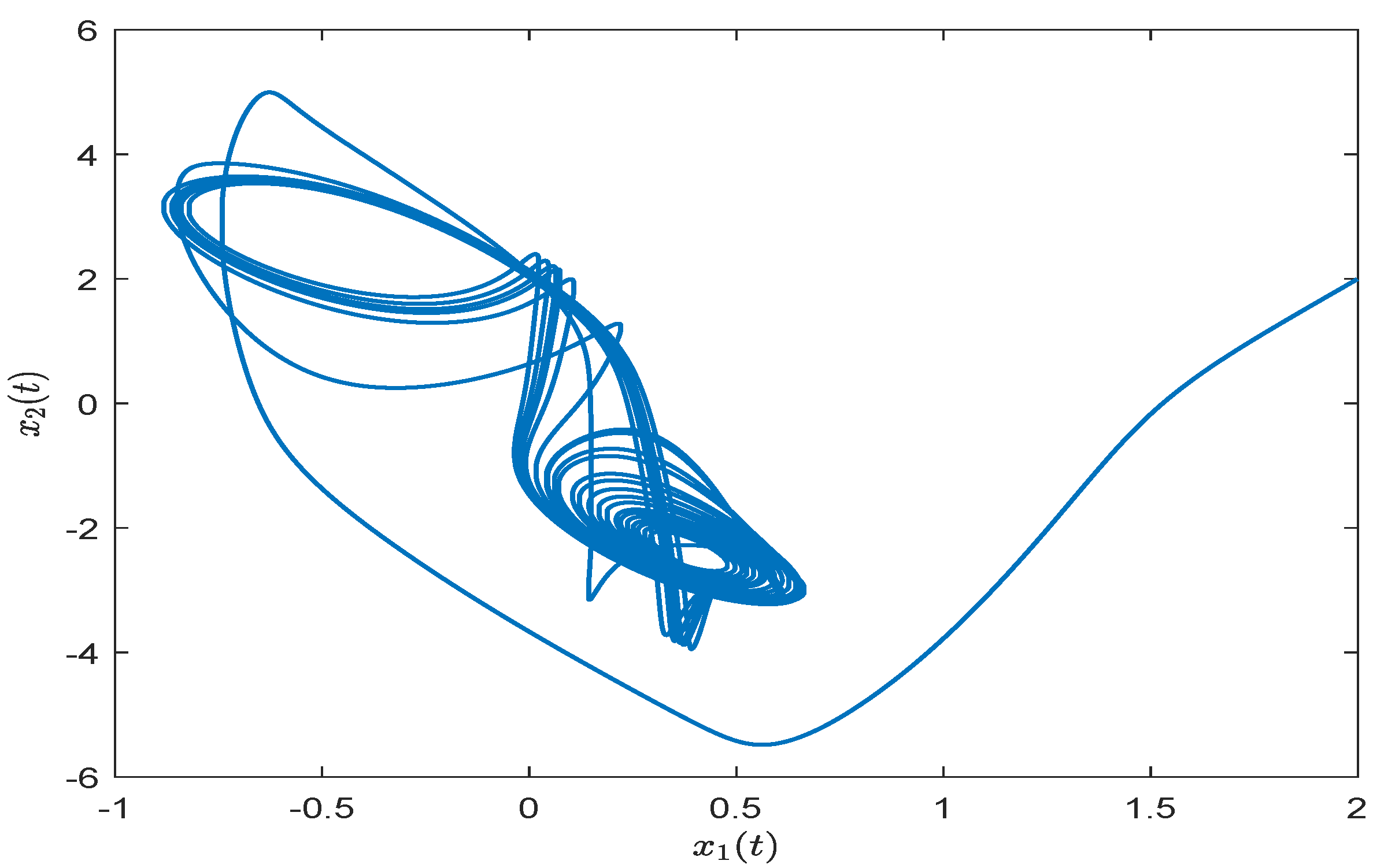
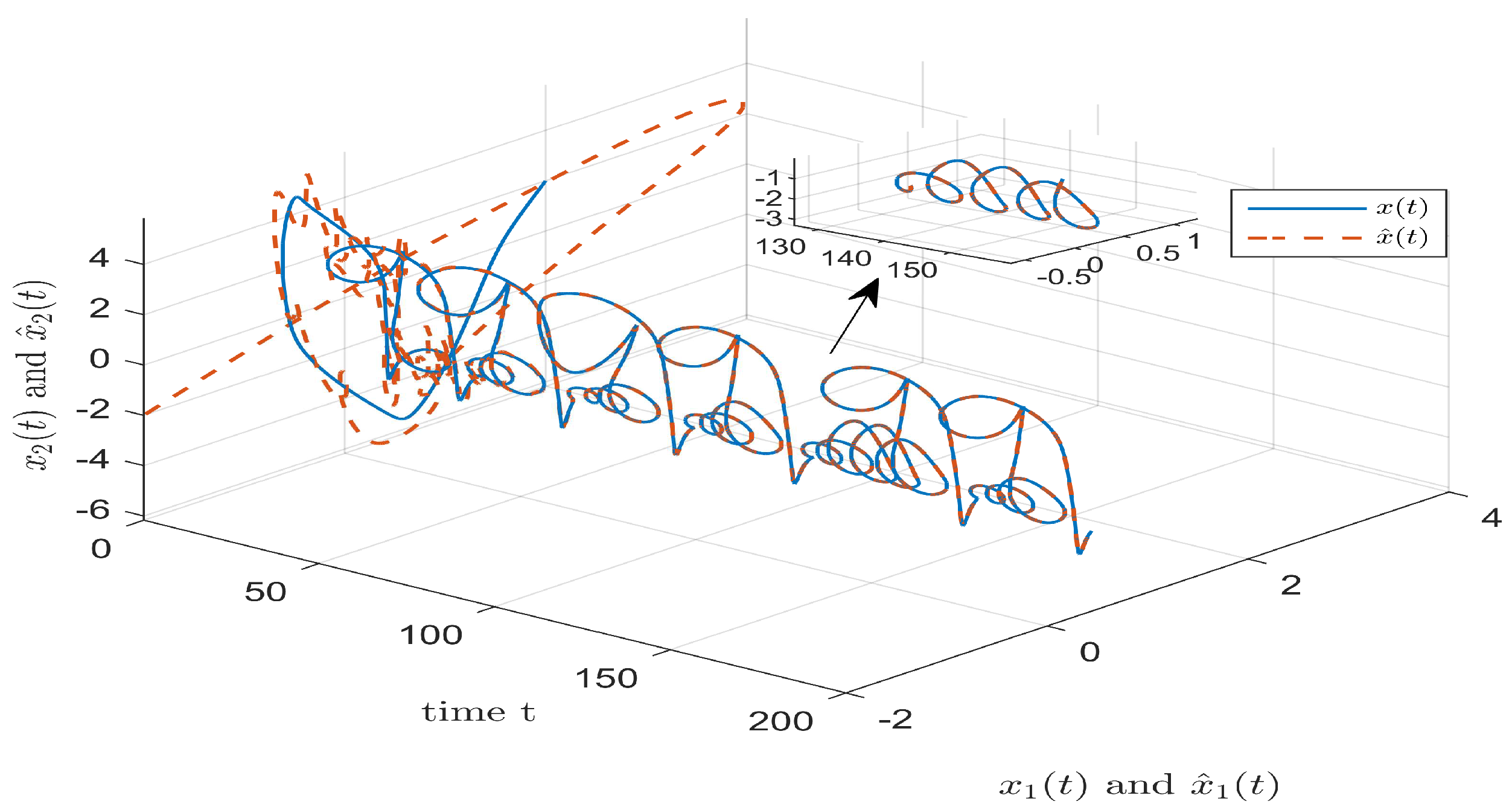
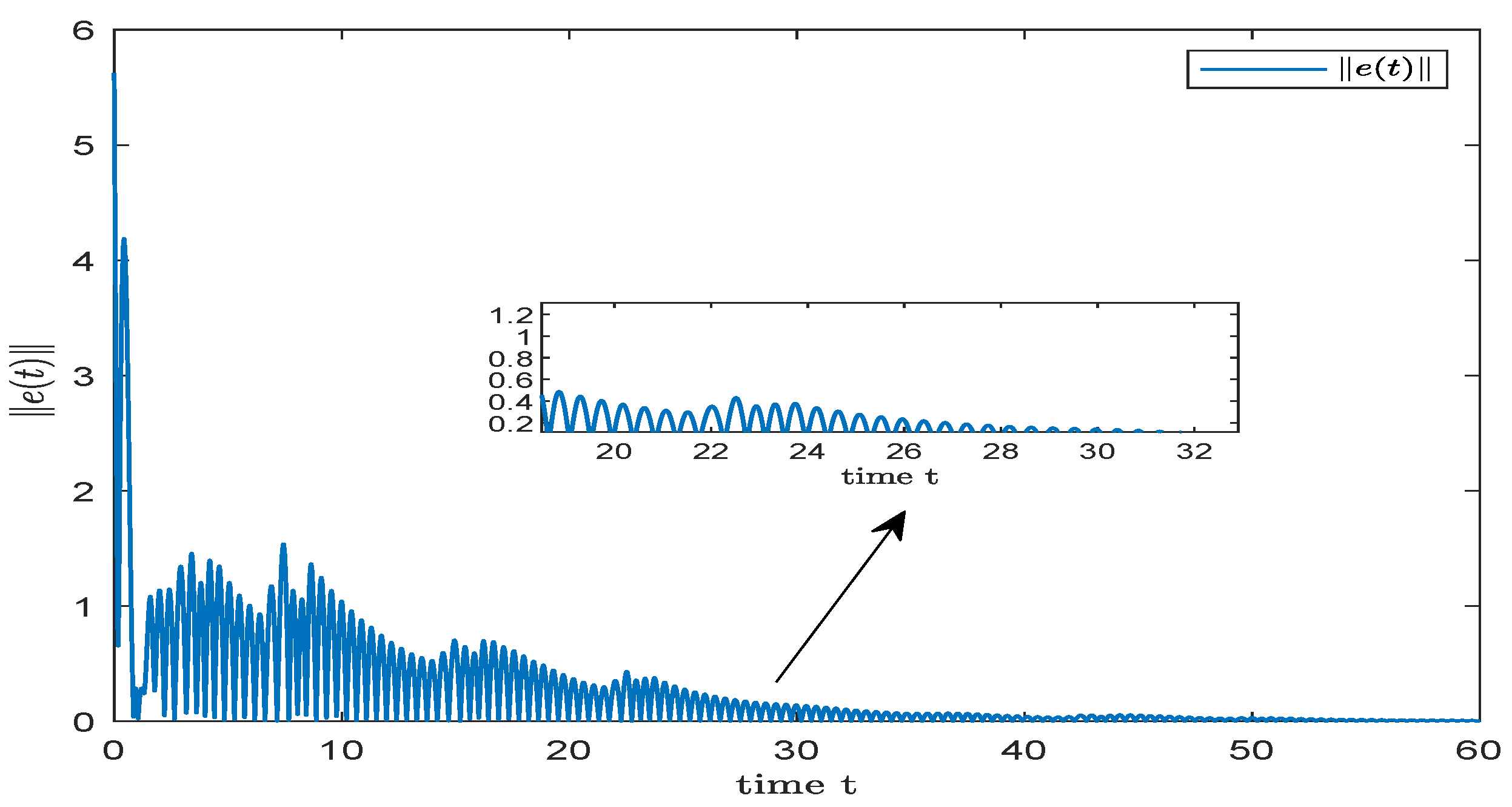
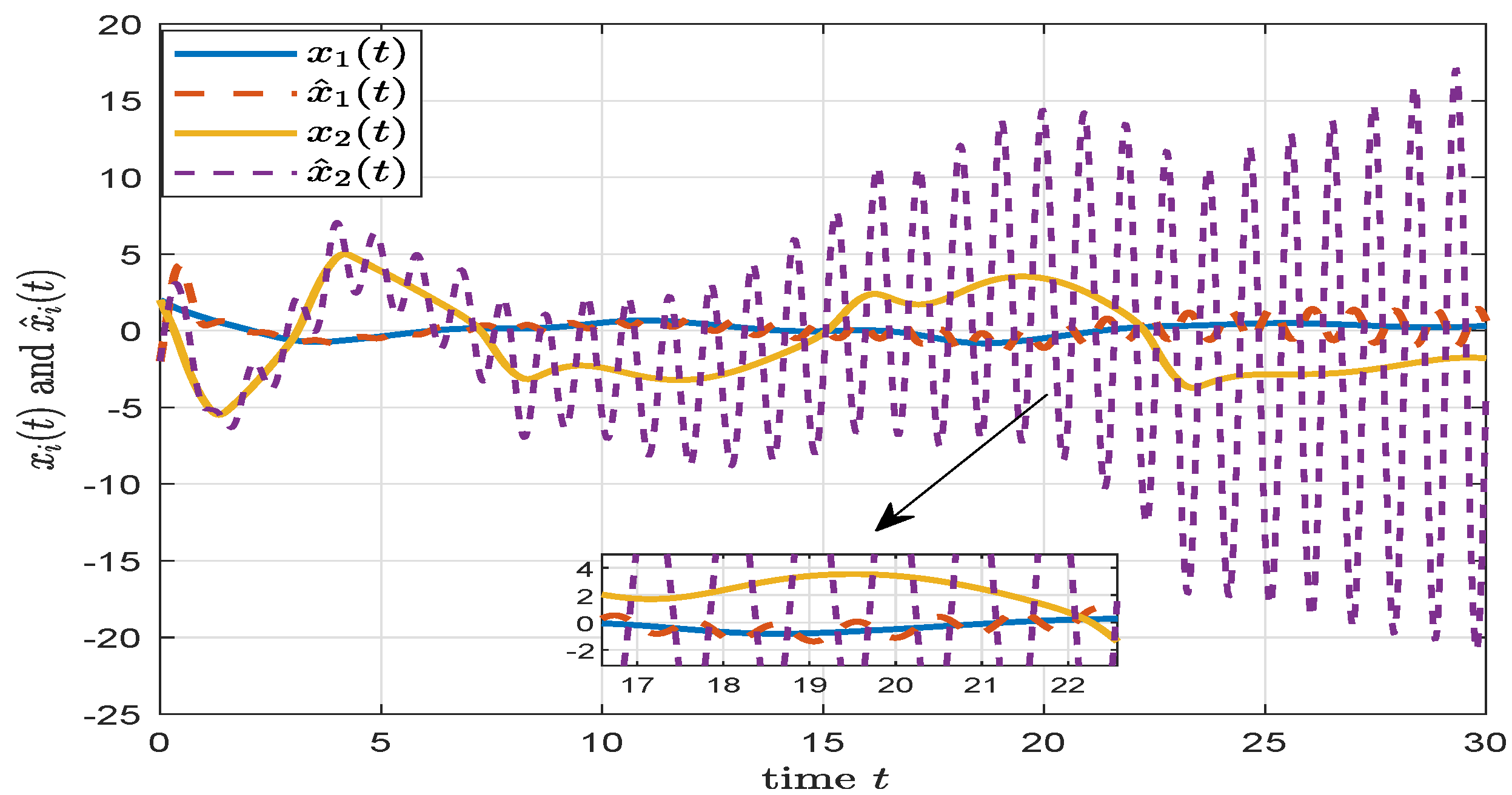
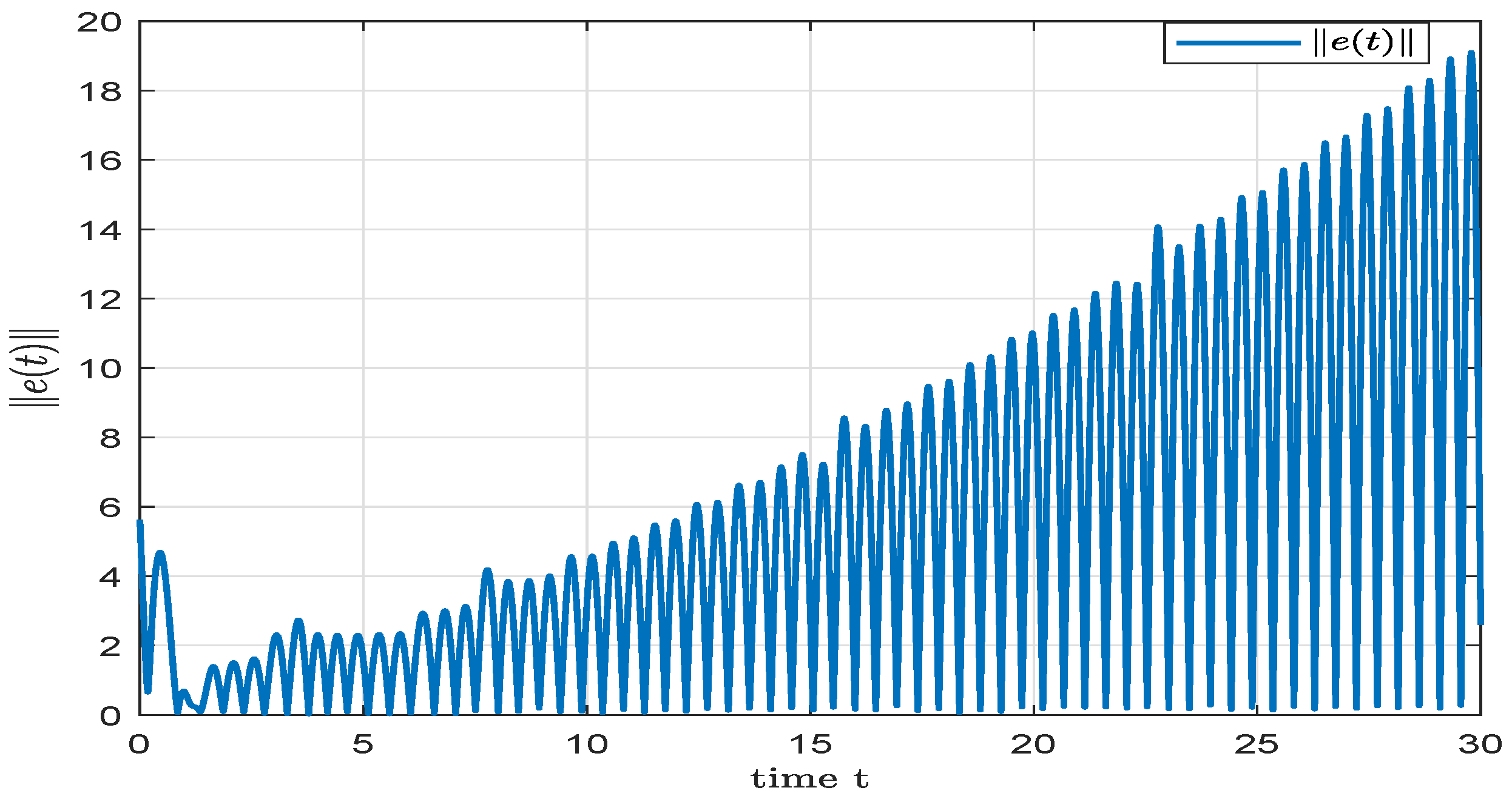
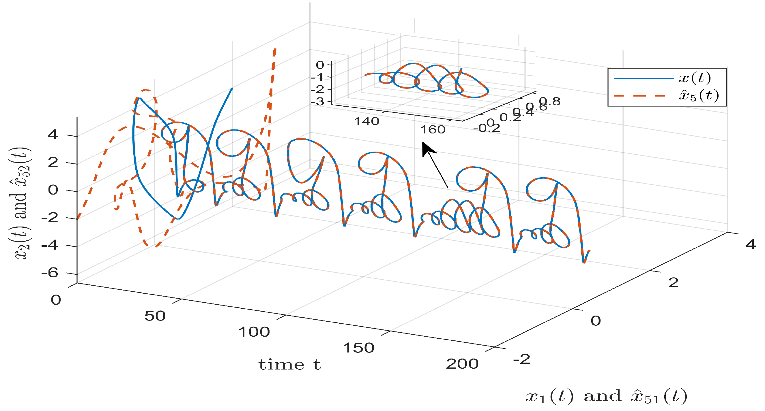
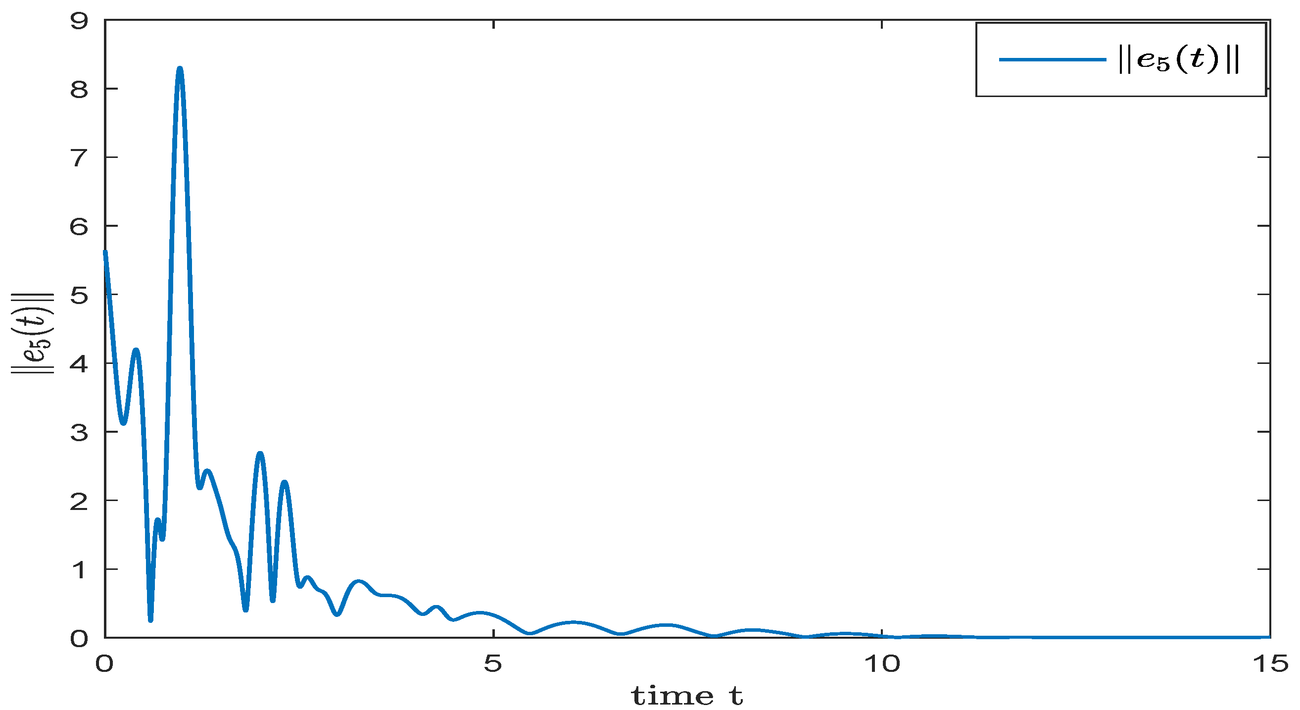
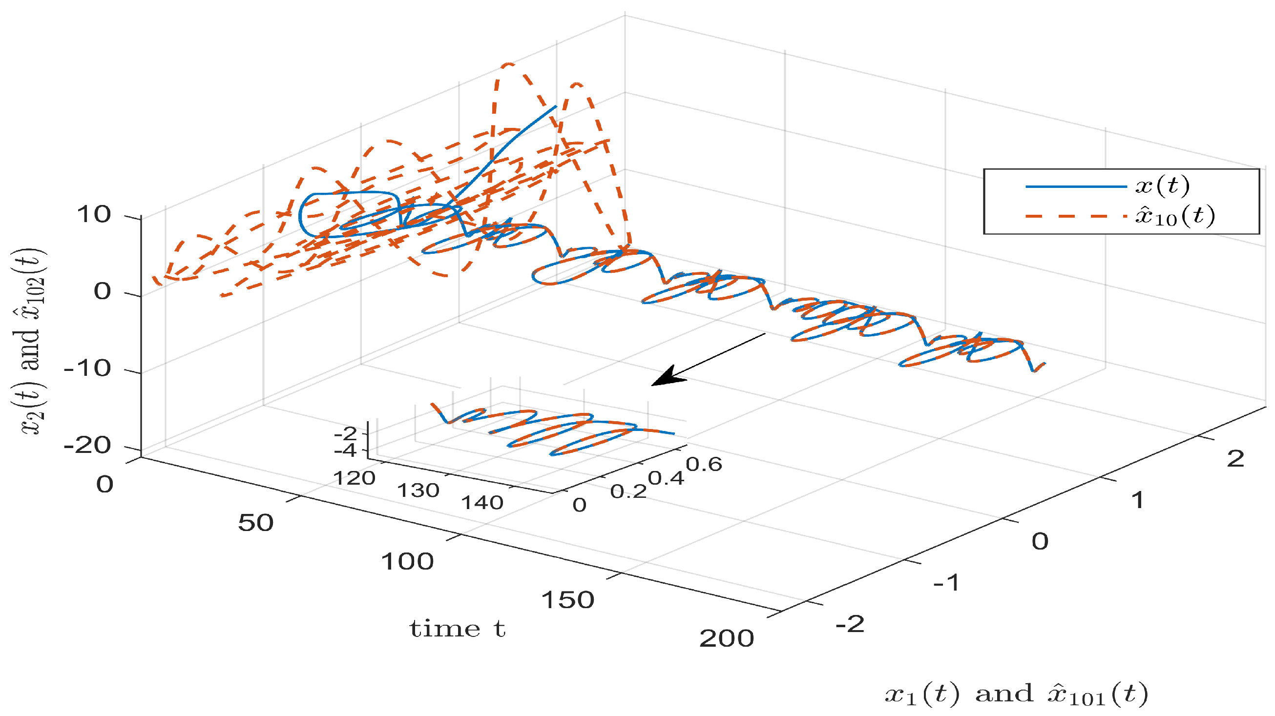
4. Numerical Simulation

This section provides a series of numerical simulations to demonstrate the efficacy of our results.

Let $x\left(t\right)={[x_1\left(t\right),x_2\left(t\right)]}^T$. Consider the RNNs (1) with the following parameters:

$$\begin{array}{cc}\hfill & A=\left[\begin{array}{cc}1& 0\\ 0& 1\end{array}\right],W_0=\left[\begin{array}{cc}2.0& -0.1\\ -5.0& 3.0\end{array}\right],W_1=\left[\begin{array}{cc}-1.5& -0.1\\ -0.2& -2.5\end{array}\right],C=\left[\begin{array}{cc}3& 0.3\\ 0.3& 3\end{array}\right],\hfill \\ \hfill & h_x=1,\varphi \left(s\right)={[2,2]}^T,f\left(x\left(t\right)\right)={[tanh\left(x_1\left(t\right)\right),tanh\left(x_2\left(t\right)\right)]}^T,\hfill \end{array}$$

where $h_y$ exists if we take the value later. It can be observed from Figure 1 that these RNNs have complex chaotic behaviors. Then, from Theorem 1, it follows that there is a nonfeasible solution to the LMI set (12) when $h^{\ast }>0.24$. Therefore, when $h_y\le 0.24$, we only use the full-order observer (6). When $h_y>0.24$, we use the cascade predictor (23).

Example 1. 

For $h_y=0.23$, assume that the initial conditions of the full-order observer $\widehat{x}$ are $\widehat{x}\left(s\right)={[-2,-2]}^T$, $s\in [-1,0)$. Then, from Theorem 1, we can obtain feasible solutions:

$$\begin{array}{c}\hfill P=\left[\begin{array}{cc}15.9540& 0.3889\\ 0.3889& 2.3080\end{array}\right],L=\left[\begin{array}{cc}-1.4728& 0.1894\\ 1.1641& -2.3357\end{array}\right].\end{array}$$

The simulation results are shown in Figure 2 and Figure 3. Figure 2 represents the trajectory profiles of $\widehat{x}\left(t\right)$ and $x\left(t\right)$, which implies the validity of our designed full-order observer (6). Figure 3 represents the converged trajectory of $\parallel e\left(t\right)\parallel =\parallel \widehat{x}\left(t\right)-x\left(t\right)\parallel$, which implies the convergence performance of the full-order observer (6). However, when $h=0.25$, it can be observed from Figure 4 and Figure 5 that the full-order observer cannot accurately estimate the state of the original system and the estimation error $\parallel e\left(t\right)\parallel$ becomes larger, since $h=0.25$ is greater than $h^{\ast }=0.24$.

Example 2. 

This example considers the case $h_y>0.24$; thus, we only use the cascade predictor (23).

(i) For $h_y=0.5$, we select $m=5$ and $h=0.1$ and assume that the initial conditions of ${\widehat{x}}_i$, $i=1,\cdots ,5$ are ${\widehat{x}}_i\left(s\right)={[-2,-2]}^T$, $s\in [-1,0)$. Then, from Theorem 2, we obtain feasible solutions:

$$\begin{array}{c}\hfill P_i=\left[\begin{array}{cc}142.1455& -3.8554\\ -3.8554& 16.5776\end{array}\right],L_i=\left[\begin{array}{cc}-1.5129& 0.1483\\ 1.5729& -2.8071\end{array}\right](i=1,\cdots 5).\end{array}$$

As illustrated in Figure 6 and Figure 7, the cascade predictor is valid and the estimation error $\parallel e_5\left(t\right)\parallel =\parallel {\widehat{x}}_5\left(t\right)-x\left(t\right)\parallel$ finally converges to 0.

(ii) For $h_y=1$, we select $m=10$ and $h=0.1$ and assume that the initial conditions of ${\widehat{x}}_i$, $i=1,\cdots ,10$ are ${\widehat{x}}_i\left(s\right)={[-1,-1]}^T$, $s\in [-1,0)$. Since the value of h is equal to the value of h in i), the observer gain $L_i$$(i=1,\cdots ,10)$ can be equal to the observer gain in (i). Then, from Figure 8 and Figure 9, it is clear that the cascade predictor is valid, and the observer error $\parallel e_{10}\left(t\right)\parallel =\parallel {\widehat{x}}_{10}\left(t\right)-x\left(t\right)\parallel$ finally converges to 0.

Example 3. 

This example will further discuss the effect of the size of the output delay on the convergence of the two predictors. The simulation results are shown in Figure 10, Figure 11 and Figure 12, and the influence of m and h on the convergence time is given in

Table 1. The convergence time for two types of predictors by setting observer error $\parallel e\parallel =0.1$.

Predictor∖${\mathit{h}}_{\mathit{y}}$		${\mathit{h}}_{\mathit{y}}=0.1$	${\mathit{h}}_{\mathit{y}}=0.2$	${\mathit{h}}_{\mathit{y}}=0.5$	${\mathit{h}}_{\mathit{y}}=1$	${\mathit{h}}_{\mathit{y}}=1.5$	${\mathit{h}}_{\mathit{y}}=2$
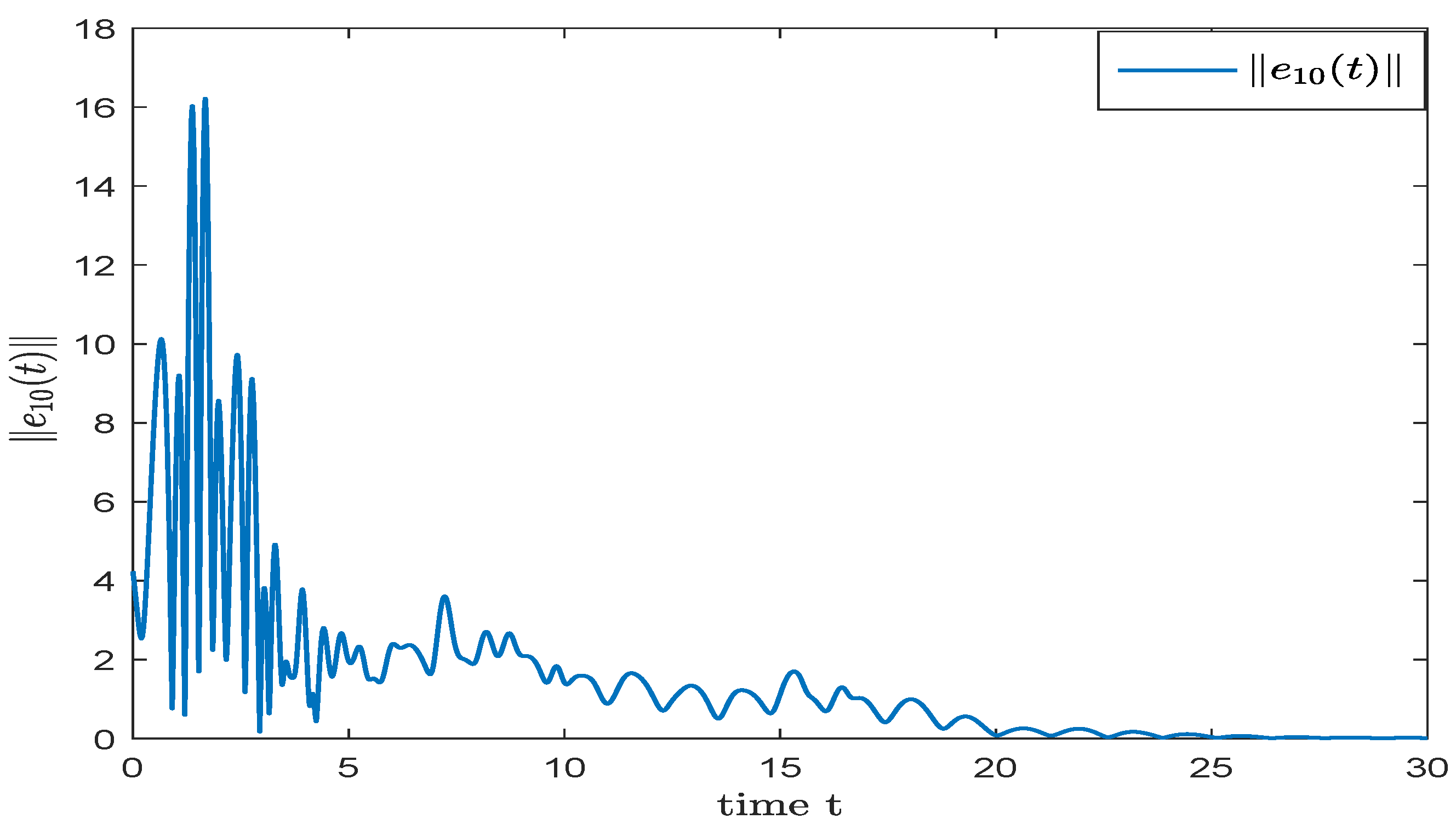
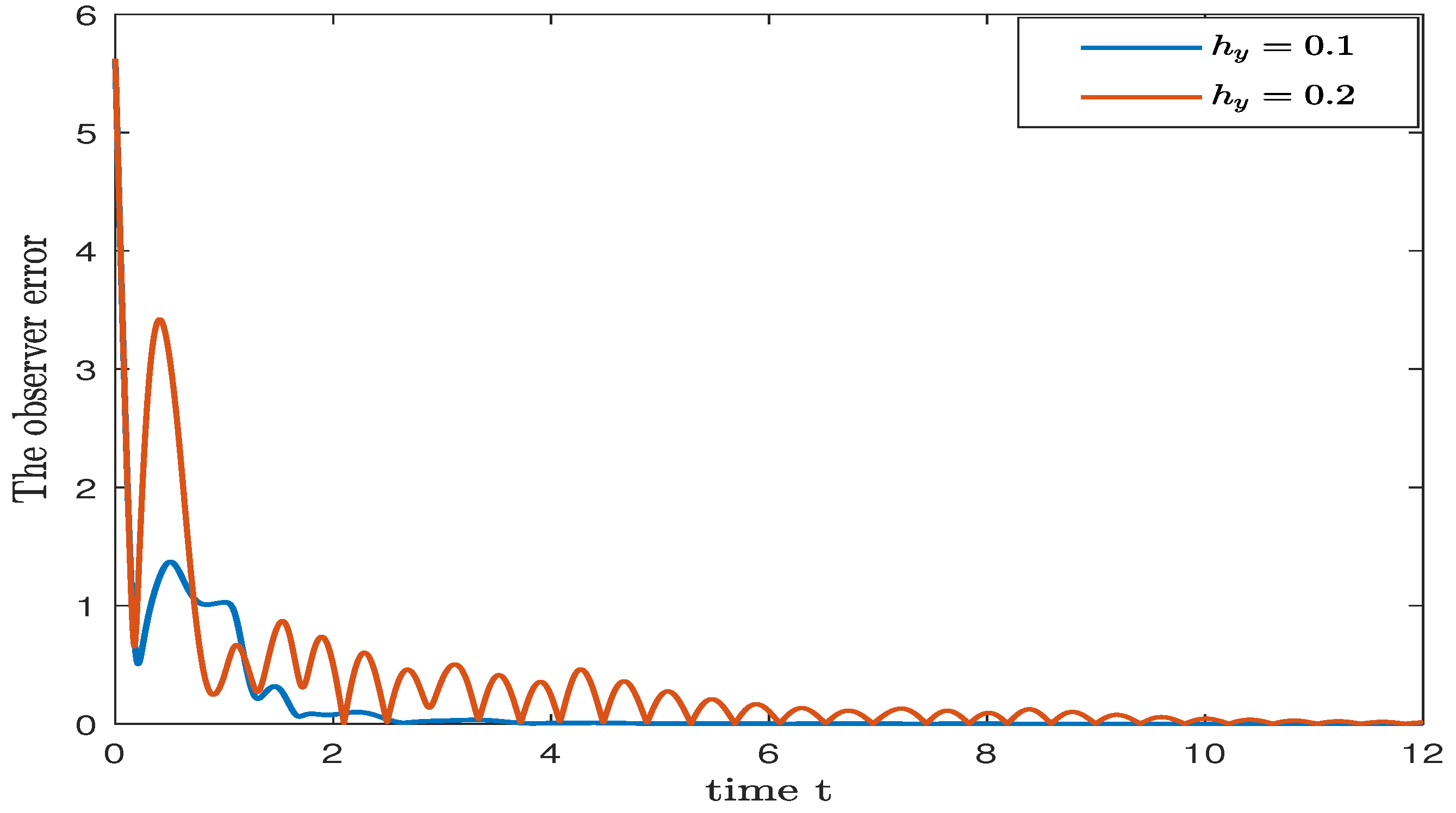
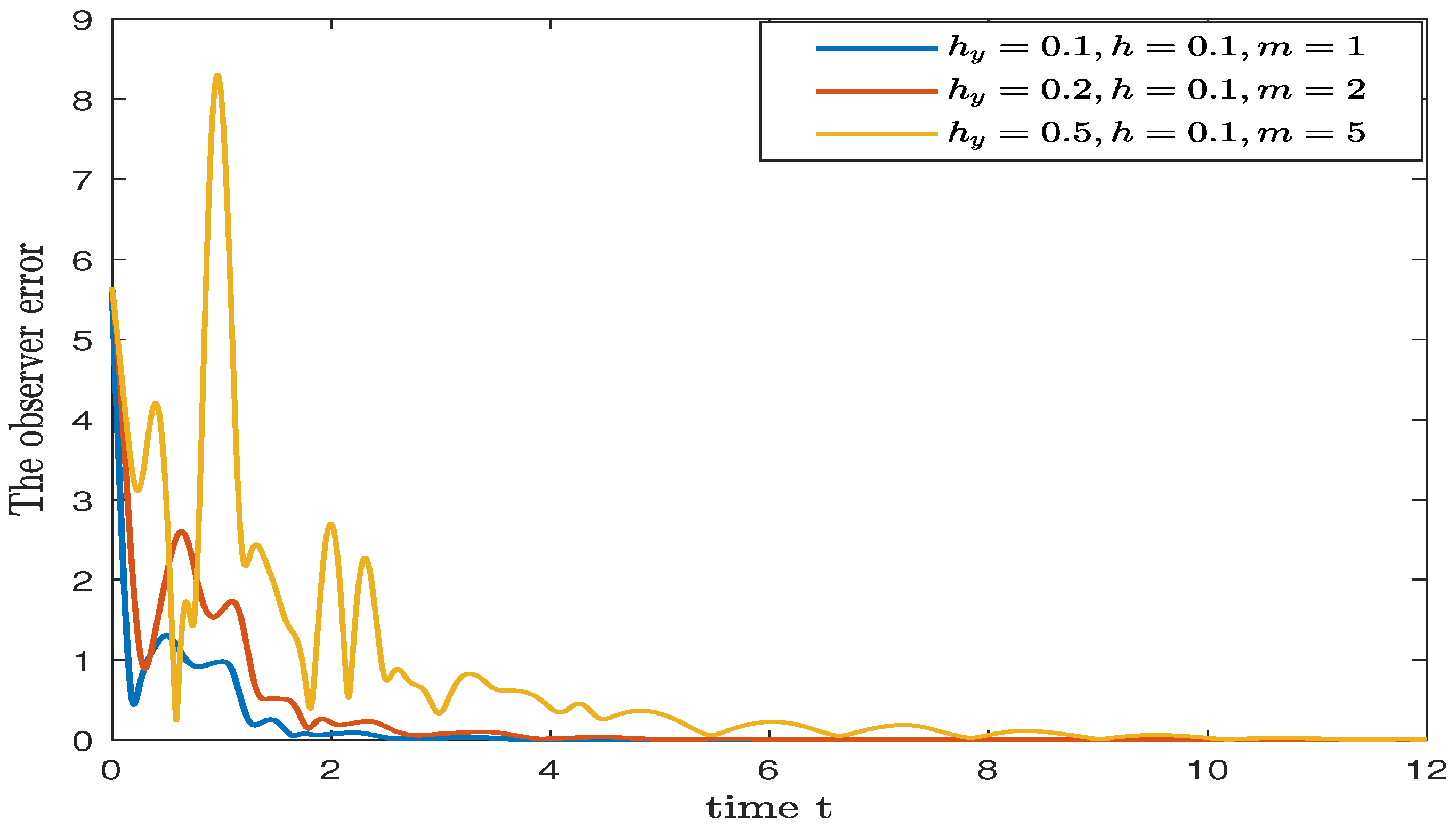
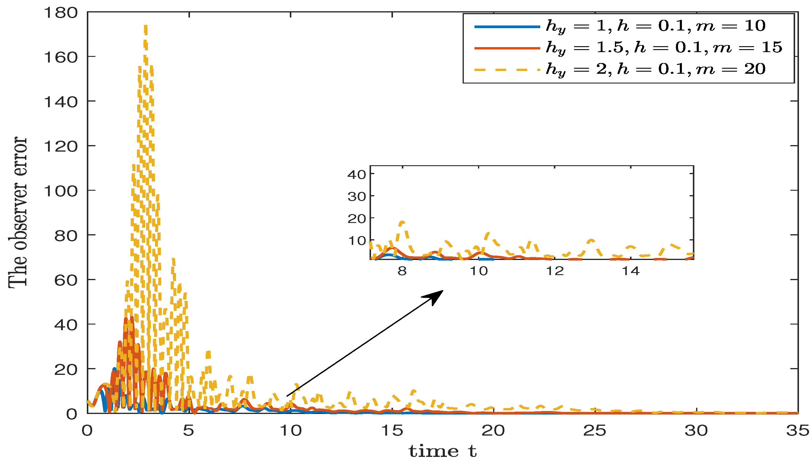
Convergence time	Simple observer	1.6	8.5	*	*	*	*
	Cascade predictor	1.8 (m = 1)	3.6 (m = 2)	9.1 (m = 5)	16.3 (m = 10)	27.4 (m = 15)	31.5 (m = 20)

, where “*" denoting the single observer is not valid ($h_y>h^{\ast }$).

From Table 1, we can clearly observe that for both predictors, the output delay is directly proportional to the convergence time, and the larger the output delay, the longer the convergence time. In addition, from the experimental results, it can be concluded that, although the cascade predictor can solve the problem of an arbitrarily large output delay, as $h_y$ increases, we will have to choose more subsystems to transmit the state information, which leads to the accumulation of error information and increases the cost of observation.

5. Conclusions

In this research, we investigate the RNNs’ state estimation by proposing an output-predicting and LPV approach. Due to the LPV approach, LKF and convex principle, several new conditions for the global asymptotic stability of the error system have been established. Compared with the traditional observer in [14,15,16,17,18,19,20], the chain-structured cascade predictor is more useful in the state estimation of neural networks. Different from [12,13,15,16,20], we use the LPV approach to convert nonlinear error dynamic systems into linear error systems, which greatly reduces the difficulty of the stability analysis. Finally, a series of numerical simulations show the effectiveness of the cascade predictor.

References

- Chua, L.; Yang, L. Cellular neural networks: Application. IEEE Trans. Circuits Syst. 1998, 35, 1273–1290. [Google Scholar] [CrossRef]
- Cichocki, A.; Unbehauen, R. Neural Networks for Optimization and Signal Processing; Wiley: Chichester, UK, 1993. [Google Scholar]
- Joya, G.; Atencia, M.; Sandoval, F. Hopfield neural networks for optimization: Study of the different dynamics. Neurocomputing 2002, 43, 219–237. [Google Scholar] [CrossRef]
- Li, W.; Lee, T. Hopfield neural networks for affine invariant matching. IEEE Trans. Neural Netw. 2001, 12, 1400–1410. [Google Scholar] [CrossRef]
- Yong, S.; Scott, P.; Nasrabadi, N. Object recognition using multilayer Hopfield neural network. IEEE Trans. Image Process. 1997, 6, 357–372. [Google Scholar] [CrossRef] [PubMed]
- Wang, Z.; Liu, L.; Shan, Q.; Zhang, H. Stability criteria for recurrent neural networks with time-varying delay based on secondary delay partitioning method. IEEE Trans. Neural Netw. Learn. Syst. 2015, 26, 2589–2595. [Google Scholar] [CrossRef] [PubMed]
- Zhang, C.; He, Y.; Jiang, L.; Wu, M. Delay-dependent stability criteria for generalized neural networks with two delay components. IEEE Trans. Neural Netw. Learn. Syst. 2014, 25, 1263–1276. [Google Scholar] [CrossRef]
- Zhang, X.; Han, Q. Global asymptotic stability analysis for delayed neural networks using a matrix-based quadratic convex approach. Neural Netw. 2014, 54, 57–69. [Google Scholar] [CrossRef] [PubMed]
- Wang, Z.; Zhang, H.; Jiang, B. LMI-based approach for global asymptotic stability analysis of recurrent neural networks with various delays and structures. IEEE Trans. Neural Netw. 2011, 22, 1032–1045. [Google Scholar] [CrossRef] [PubMed]
- Liu, Y.J.; Lee, S.M.; Kwon, O.M.; Park, J.H. New approach to stability criteria for generalized neural networks with interval time-varying delays. Neurocomputing 2015, 149, 1544–1551. [Google Scholar] [CrossRef]
- Wu, Z.; Shi, P.; Su, H.; Chu, J. Delay-dependent stability analysis for switched neural networks with time-varying delay. IEEE Trans. Syst. Man Cybern. Part B (Cybern.) 2011, 41, 1522–1530. [Google Scholar] [CrossRef]
- Zhu, Q.; Cao, J. Stability of Markovian jump neural networks with impulse control and time varying delays. Nonlinear Anal. Real World Appl. 2012, 13, 2259–2270. [Google Scholar] [CrossRef]
- Wang, Z.; Ho, D.W.C.; Liu, X. State estimation for delayed neural networks. IEEE Trans. Neural Netw. 2005, 16, 279–284. [Google Scholar] [CrossRef] [PubMed]
- Wang, Z.; Liu, R.; Liu, Y. State estimation for jumping recurrent neural networks with discrete and distributed delays. Neural Netw. 2009, 22, 41–48. [Google Scholar] [CrossRef] [PubMed]
- Wang, Z.; Wang, J.; Wu, Y. State estimation for recurrent neural networks with unknown delays: A robust analysis approach. Neurocomputing 2017, 227, 29–36. [Google Scholar] [CrossRef]
- Huang, H.; Feng, G.; Cao, J. Robust state estimation for uncertain neural networks with time-varying delay. IEEE Trans. Neural Netw. 2008, 19, 1329–1339. [Google Scholar] [CrossRef]
- Huang, H.; Feng, G.; Cao, J. State estimation for static neural networks with time-varying delay. Neural Netw. 2010, 23, 1202–1207. [Google Scholar] [CrossRef]
- Ren, J.; Zhu, H.; Zhong, S.; Ding, Y.; Shi, K. State estimation for neural networks with multiple time delays. Neurocomputing 2015, 151, 501–510. [Google Scholar] [CrossRef]
- Liu, M.; Chen, H. H∞ state estimation for discrete-time delayed systems of the neural network type with multiple missing measurements. IEEE Trans. Neural Netw. Learn. Syst. 2015, 26, 2987–2998. [Google Scholar] [CrossRef]
- Guo, M.; Zhu, S.; Liu, X. Observer-based state estimation for memristive neural networks with time-varying delay. Knowl.-Based Syst. 2022, 246, 108707. [Google Scholar] [CrossRef]
- Beintema, G.I.; Schoukens, M.; Toth, R. Deep subspace encoders for nonlinear system identification. Automatica 2023, 156, 111210. [Google Scholar] [CrossRef]
- Germani, A.; Manes, C.; Pepe, P. A new approach to state observation of nonlinear systems with delayed output. IEEE Trans. Autom. Control 2002, 47, 96–101. [Google Scholar] [CrossRef]
- Ahmed-Ali, T.; Cherrier, E.; Lamnabhi-Lagarrigue, F. Cascade high gain predictors for a class of nonlinear systems. IEEE Trans. Autom. Control 2012, 57, 224–229. [Google Scholar] [CrossRef]
- Farza, M.; M’Saad, M.; Menard, T.; Fall, M.L.; Gehan, O.; Pigeon, E. Simple cascade observer for a class of nonlinear systems with long output delays. IEEE Trans. Autom. Control 2015, 60, 3338–3343. [Google Scholar] [CrossRef]
- Farza, M.; Hernandez-Gonzalez, O.; Menard, T.; Targui, B.; M’Saad, M.; Astorga-Zaragoza, C.M. Cascade observer design for a class of uncertain nonlinear systems with delayed outputs. Automatica 2018, 89, 125–134. [Google Scholar] [CrossRef]
- Zemouche, A.; Boutayeb, M. On LMI conditions to design observers for Lipschitz nonlinear systems. Automatica 2013, 49, 585–591. [Google Scholar] [CrossRef]
- Adil, A.; Hamaz, A.; N’Doye, I.; Zemouche, A.; Laleg-Kirati, T.M.; Bedouhene, F. On high-gain observer design for nonlinear systems with delayed output measurements. Automatica 2022, 141, 11281. [Google Scholar] [CrossRef]
- Huang, H.; Huang, T.; Chen, X.; Qian, C. Exponential stabilization of delayed recurrent neural networks: A state estimation based approach. Neural Netw. 2013, 48, 153–157. [Google Scholar] [CrossRef] [PubMed]
- Zhang, Z.; He, Y.; Zhang, C.; Wu, M. Exponential stabilization of neural networks with time-varying delay by periodically intermittent control. Neurocomputing 2016, 207, 469–475. [Google Scholar] [CrossRef]
- Huang, H.; Feng, G. Delay-dependent h∞ and generalized h2 filtering for delayed neural networks. IEEE Trans. Circuits Syst. Regul. Pap. 2009, 56, 846–857. [Google Scholar] [CrossRef]
- Gonzalez, A. Improved results on stability analysis of time-varying delay systems via delay partitioning method and Finsler’s lemma. J. Frankl. Inst. 2022, 359, 7632–7649. [Google Scholar] [CrossRef]
- Moon, Y.S.; Park, P.; Kwon, W.H.; Lee, Y.S. Delay-dependent robust stabilization of uncertain state-delayed systems. Int. J. Control 2001, 74, 1447–1455. [Google Scholar] [CrossRef]
- Gu, K.L.; Kharitonov, V.; Chen, J. Stability of Time-Delay Systems; Springer: Berlin, Germany, 2003. [Google Scholar]
- Body, S.; Ghaoui, L.E.; Feron, E.; Balakrishnan, V. Linear Matrix Inequalities in System and Control Theory; SIAM: Philadelphia, PA, USA, 1994. [Google Scholar]
- Khalil, H.K. Nonlinear Systems; Prentice-Hall: Englewood Cliffs, NJ, USA, 2002. [Google Scholar]