Modelization of Low-Cost Maneuvers for an Areostationary Preliminary Mission Design

Abstract

The aim of this paper is to analyze the determination of interplanetary trajectories from Earth to Mars to evaluate the cost of the required impulse magnitudes for an areostationary orbiter mission design. Such analysis is first conducted by solving the Lambert orbital boundary value problem and studying the launch and arrival conditions for various date combinations. Then, genetic algorithms are applied to investigate the minimum-energy transfer orbit. Afterwards, an iterative procedure is used to determine the heliocentric elliptic transfer orbit that matches at the entry point of Mars’s sphere of influence with an areocentric hyperbolic orbit imposing specific conditions on inclination and periapsis radius. Finally, the maneuvers needed to obtain an areostationary orbit are numerically computed for different objective condition values at the Mars entry point to evaluate an areostationary preliminary mission cost for further study and characterization. Results show that, for the dates of the minimum-energy Earth–Mars transfer trajectory, a low value for the maneuvers to achieve an areostationary orbit is obtained for an arrival hyperbola with the minimum possible inclination and a capture into an elliptical trajectory with a low periapsis radius and an apoapsis at the stationary orbit. For a 2026 mission with a TOF of 304 for the minimum-energy Earth–Mars transfer trajectory, for a capture with a periapsis of 300 km above the Mars surface the value achieved will be 2.083 km/s.

1. Introduction

Small relay satellites in areostationary orbit are considered the most efficient candidates to support the telecommunication needs in the 2020s [1,2,3,4,5,6,7]. Areostationary orbiters, like geostationary satellites for Earth [8,9], can provide continuous access at very high data rates to remotely supervise a significant population of probes and robotic missions on the Martian surface. The determination of transfer trajectories from Earth to Mars aimed at lowering costs in terms of impulses has become a key factor in mission planning, allowing for larger payloads to be transported at a minimum energy cost.

In this work, we analyze the design of an interplanetary Earth–Mars transfer to reach the areostationary orbit with the minimum impulsive maneuvers cost. Several authors have studied the optimization of interplanetary trajectories: in [10,11] transfer trajectories to the Moon and Jupiter, respectively, passing close to a Lagrangian point, are considered; in [12], a method is developed to obtain approximate near-optimal low-thrust interplanetary transfers using solar electric propulsion spacecraft; in [13], the optimization is performed with a cost function with variable coefficients; in [14], launch constraints are imposed for the optimization. We derive the heliocentric elliptic transfer characterizing the launch windows using an heuristic optimization method for determining an optimal time of flight (TOF) that minimizes the characteristic energies [15,16]. We will analyze the sensibility of this parameter in the optimization of impulsive maneuvers.

The first step consists in solving the Lambert problem [17] for various combinations of departure and arrival dates. Departure characteristic energy and hyperbolic arrival velocity plots are usually examined to investigate possible transfer windows [18]. We use genetic algorithms [19] to simultaneously minimize these two key parameters within these launch windows, comparing their performance.

Then, we match this interplanetary transfer with an entry hyperbola around Mars. The classic patched conic problem has been used to achieve a continuous trajectory composed of the trajectory between two planets and the planetocentric trajectory [20,21,22,23,24]. We use the iterative procedure [25] with imposed conditions on the periapsis distance, the arrival hyperbolic inclination, and a fixed radius for the Mars sphere of influence (SOI), and analyze the changes in the B-plane [26] due to the variations in the arrival asymptote direction. This iterative procedure enables the evaluation of these selected parameters in order to minimize fuel consumption for planning an areostationary mission. Once the fully matched trajectory to arrive at Mars is obtained, the maneuvers necessary to capture the orbiter and to place it in the areostationary orbit are analyzed.

The paper is organized as follows. In Section 2, we describe the dynamical model of the minimum-energy launch window problem. The determination of the Earth–Mars transfer trajectory with imposed hyperbolic arrival trajectory conditions is presented in Section 3. Section 4 describes the maneuvers performed to capture the spacecraft into an areostationary orbit and the numerical simulations to evaluate these maneuvers for different conditions. Finally, in Section 5, we briefly summarize the main conclusions.

2. Minimum-Energy Launch Window for Earth–Mars Transfer Trajectories

We first analyze the determination of interplanetary trajectories from Earth to Mars by minimizing the required energy at Earth departure and Mars arrival. We assume point mass gravitational forces for Earth and Mars within their respective spheres of influence and an unperturbed Keplerian orbit around the Sun.

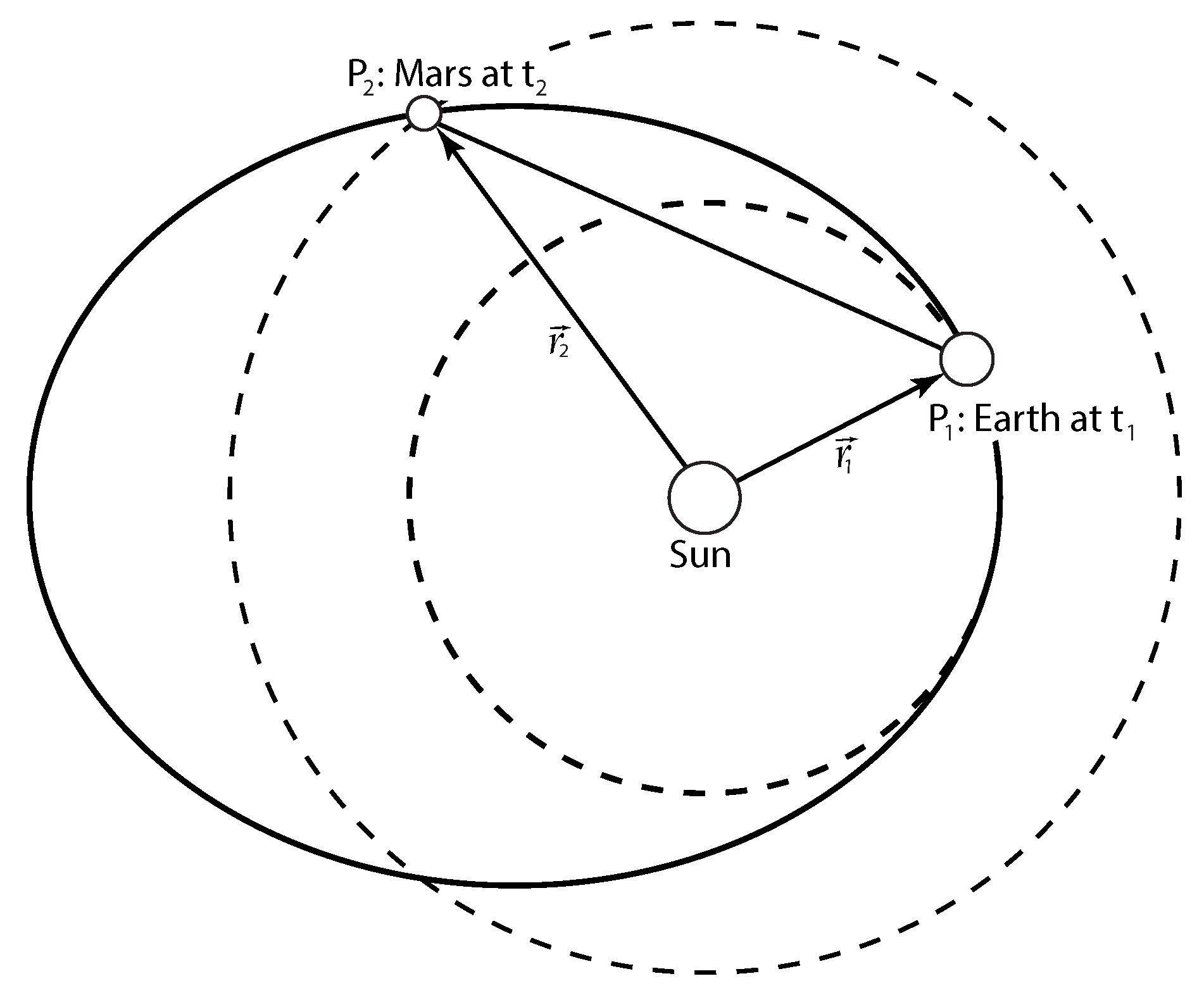
The key parameters commonly used [27,28] to analyze the Earth–Mars mission launch opportunities are the characteristic energy at departure from Earth, $C_3=V_{{\infty }_{\mathrm{E}}}^2$, the hyperbolic excess velocity to escape from Earth, $V_{{\infty }_{\mathrm{E}}}$, and Mars arrival hyperbolic excess velocity, $V_{{\infty }_{\mathrm{M}}}$. In order to obtain these two parameters, it is necessary to first solve the Lambert orbital boundary value problem for the heliocentric spacecraft position, ${\mathbf{r}}_{s_{\mathrm{S}}}$,

$${\ddot{\mathbf{r}}}_{s_{\mathrm{S}}}=-{\mu }_S\frac{{\mathbf{r}}_{s_{\mathrm{S}}}}{r_{s_{\mathrm{S}}}^3},$$

(1)

constrained by two points, $P_1$ and $P_2$, and an elapsed TOF, $t_2=t_1+\mathrm{TOF}$, as illustrated in Figure 1,

$$\begin{array}{ccc}\hfill {\mathbf{r}}_{s_{\mathrm{S}}}\left(t_1\right)& =& {\mathbf{r}}_{\mathrm{E}},\hfill \end{array}$$

(2)

$$\begin{array}{ccc}\hfill {\mathbf{r}}_{s_{\mathrm{S}}}\left(t_2\right)& =& {\mathbf{r}}_{\mathrm{M}},\hfill \end{array}$$

(3)

where ${\mathbf{r}}_{\mathrm{E}}$ and ${\mathbf{r}}_{\mathrm{M}}$ are the heliocentric position vectors for the Earth at $t_1$ and Mars at $t_2$, respectively.

The solution to the Lambert problem results in an elliptic conic section connecting $P_1$ and $P_2$. We consider the shortcut solution that satisfies the boundary conditions, based on the iterative procedure, choosing the time transfer function introduced by Lancaster [29] as parameter for the iteration. The solution results in an elliptic conic section connecting $P_1$ and $P_2$, with departure and arrival velocities, ${\mathbf{V}}_{s_{\mathrm{S}1}}$ and ${\mathbf{V}}_{s_{\mathrm{S}2}}$, at $t_1$ and $t_2$, respectively.

For each Earth departure and Mars arrival combination of dates, ${\mathbf{V}}_{{\infty }_{\mathrm{E}}}$ and ${\mathbf{V}}_{{\infty }_{\mathrm{M}}}$ change as ${\mathbf{V}}_{s_{\mathrm{S}1}}$ and ${\mathbf{V}}_{s_{\mathrm{S}2}}$ change according to

$$\begin{array}{c}\hfill {\mathbf{V}}_{{\infty }_E}={\mathbf{V}}_{s_{\mathrm{S}1}}-{\mathbf{V}}_{E_{\mathrm{S}1}},\end{array}$$

(4)

$$\begin{array}{c}\hfill {\mathbf{V}}_{{\infty }_M}={\mathbf{V}}_{s_{\mathrm{S}2}}-{\mathbf{V}}_{M_{\mathrm{S}2}},\end{array}$$

(5)

where ${\mathbf{V}}_{E_{\mathrm{S}1}}$ and ${\mathbf{V}}_{M_{\mathrm{S}2}}$ are the heliocentric velocity vectors for the Earth at $t_1$ and Mars at $t_2$, respectively.

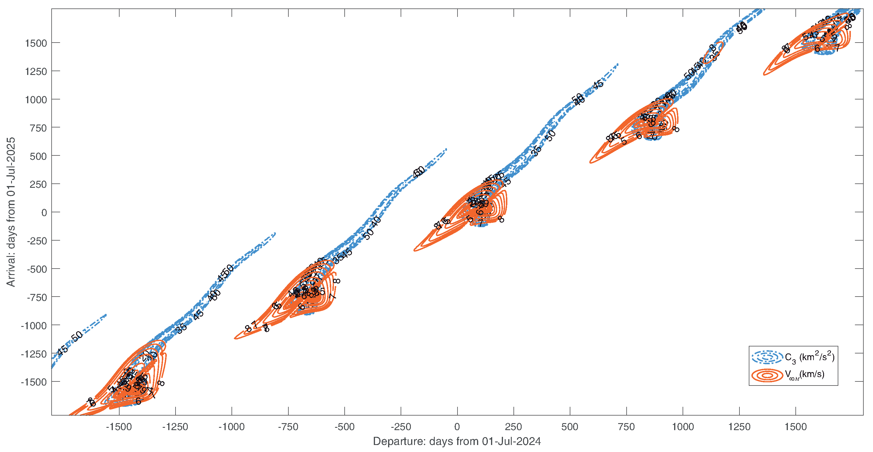
To analyze launch and arrival window opportunities, we first focus on data visualization [15,18] of the departure characteristic energy $C_3$ and the hyperbolic arrival velocity $V_{{\infty }_M}$ for various combinations of departure and arrival dates. We use Matlab software available from [30] to solve the Lambert problem, first obtaining a reduced launch window for the minimum-energy solution. The porkchop plots [31,32] shown in Figure 2 depict the contour lines of constant $C_3$ in ${\mathrm{km}}^2/{\mathrm{s}}^2$ and $V_{{\infty }_M}$ in $\mathrm{km}/\mathrm{s}$ for the 2019–2029 departure and the 2020–2030 arrival time frames. It is possible to observe that the launch and arrival windows that give the minimum values approximately repeat every Mars synodic period of about 780 days. 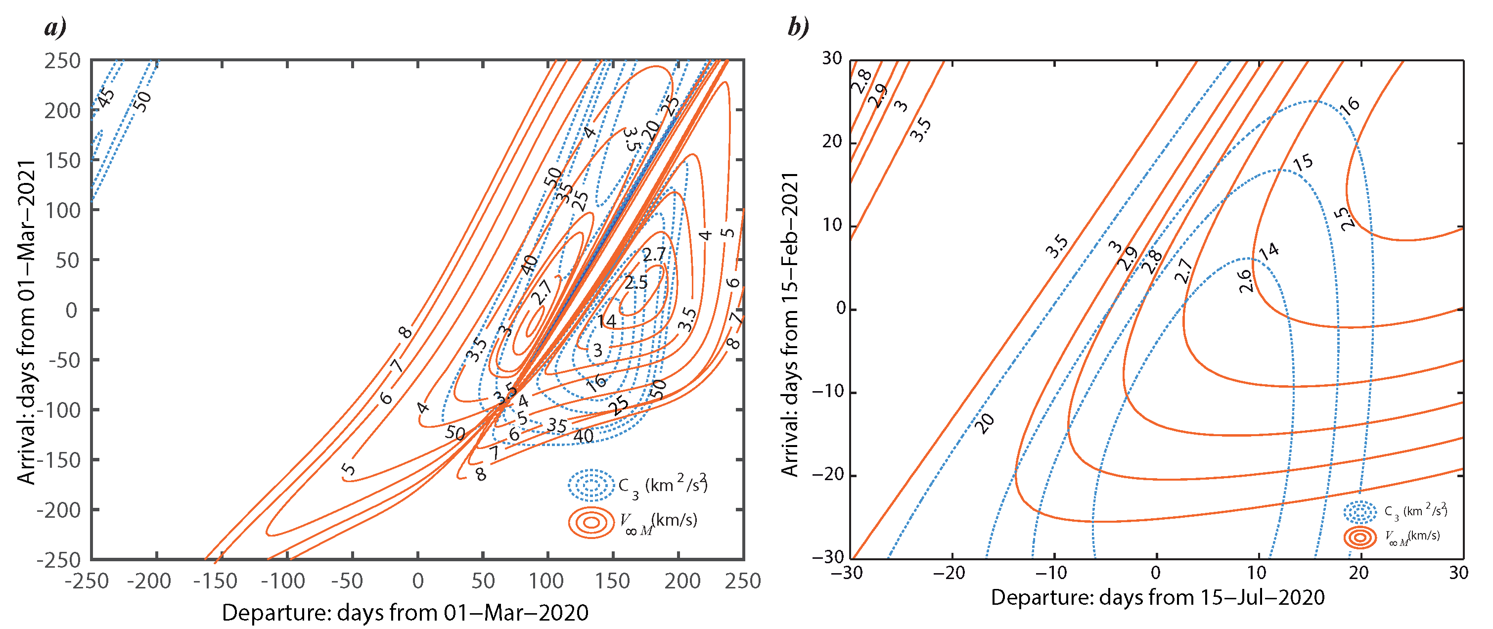In more detail, Figure 3a shows the departure characteristic energy and hyperbolic arrival velocity contour plots for the Earth–Mars transfer covering 27 months, from 1 July 2019 to 1 November 2021, and Figure 3b presents these plots for the departure window on July 2020 and the arrival window on February 2021.

Now, we search for the solution minimizing the equation:

$$C=C_3+V_{{\infty }_M}.$$

(6)

The minimum C in Equation (6) tends to give lower values of the impulsive maneuvers required, first to obtain an Earth escape velocity, and after, at the Mars arriving hyperbolic orbit, to reduce the hyperbolic excess velocity to capture the probe.

To minimize Equation (6), applied to the reduced windows previously estimated from porkchop plots, we now use a Matlab optimizer [33] that includes a library dedicated to genetic algorithms with different implementations of selection and crossover functions (see [19]). In order to analyze the accuracy of the genetic algorithms when applied to this problem, we compare the performance of the Remainder and the Stochastic Uniform functions as selection functions to select the individuals that contribute to the population at the next generation, and the Heuristic, the Scattered, and the Single point rules as crossover functions to combine two individuals to form the next generation for populations of 100, 500, and 2000 individuals.

Table 1. Simulation scenarios in a launch window in 2020 to compare the genetic algorithm performances minimizing the cost function, $C=C_3+V_{{\infty }_M}$, of the required $C_3$ energy and the arrival velocity, $V_{{\infty }_M}$.

Pop.	Crossover	Selection	CPU	Departure	TOF	${\mathit{C}}_3$	${\mathit{V}}_{{\mathit{\infty }}_{\mathit{M}}}$	C
			Time (s)	Time	(Days)	$\mathbf{(}{\mathbf{km}}^{\mathbf{2}}\mathbf{/}{\mathbf{s}}^{\mathbf{2}}\mathbf{)}$	$\mathbf{(}\mathbf{km}\mathbf{/}\mathbf{s}\mathbf{)}$
Departure Date 20 July 2020
100	Heuristic	remainder	10.86	01:19:08	196.9397	13.2216	2.7681	15.9897
		stoch. unif.	10.36	01:05:27	196.9253	13.2212	2.7685	15.9897
	Scattered	remainder	10.30	01:04:01	196.9501	13.2213	2.7684	15.9897
		stoch. unif.	10.49	01:01:17	196.9281	13.2212	2.7685	15.9897
	Single pt	remainder	10.14	01:06:02	196.9657	13.2218	2.7679	15.9897
		stoch. unif.	10.35	01:14:40	196.9566	13.2217	2.7680	15.9897
500	Heuristic	remainder	48.30	01:06:27	196.9288	13.2212	2.7685	15.9897
		stoch. unif.	47.86	01:13:05	196.9420	13.2215	2.7682	15.9897
	Scattered	remainder	48.31	01:12:22	196.9420	13.2215	2.7682	15.9897
		stoch. unif.	47.60	01:21:17	196.9537	13.2218	2.7679	15.9897
	Single pt	remainder	47.32	01:24:10	196.9407	13.2217	2.7681	15.9898
		stoch. unif.	47.19	01:16:41	196.9450	13.2216	2.7681	15.9897
2000	Heuristic	remainder	188.06	01:04:09	196.9393	13.2214	2.7683	15.9897
		stoch. unif.	186.57	01:07:45	196.9332	13.2213	2.7684	15.9897
	Scattered	remainder	222.98	01:16:41	196.9450	13.2216	2.7681	15.9897
		stoch. unif.	229.03	01:10:38	196.9361	13.2214	2.7683	15.9897
	Single pt	remainder	238.38	01:08:54	196.9343	13.2214	2.7683	15.9897
		stoch. unif.	237.49	01:26:54	196.9480	13.2218	2.7679	15.9897

summarizes the key results to compare the genetic algorithms performances. It can be concluded that the considered selection and crossover functions do not significantly change the results. CPU time depends on the population size, leading to equivalent results.

Moreover, the results in Table 1 are in agreement with the trajectories defined by the different missions launched in the year 2020. The Mars 2020 mission (EEUU) [34] was launched on 30 July 2020, and its rover, the Perseverance rover, landed on 18 February 2021, with TOF = 203 days; The Tianwen-1 mission (China) [35] was launched on 23 July 2020 and arrived in Mars on 10 February 2021, with a TOF of 202 days. The Emirates Mars Mission (UAE) [36] was launched on 19 July 2020, and arrived at the orbit around Mars on 9 February 2021, with a TOF of 205 days.

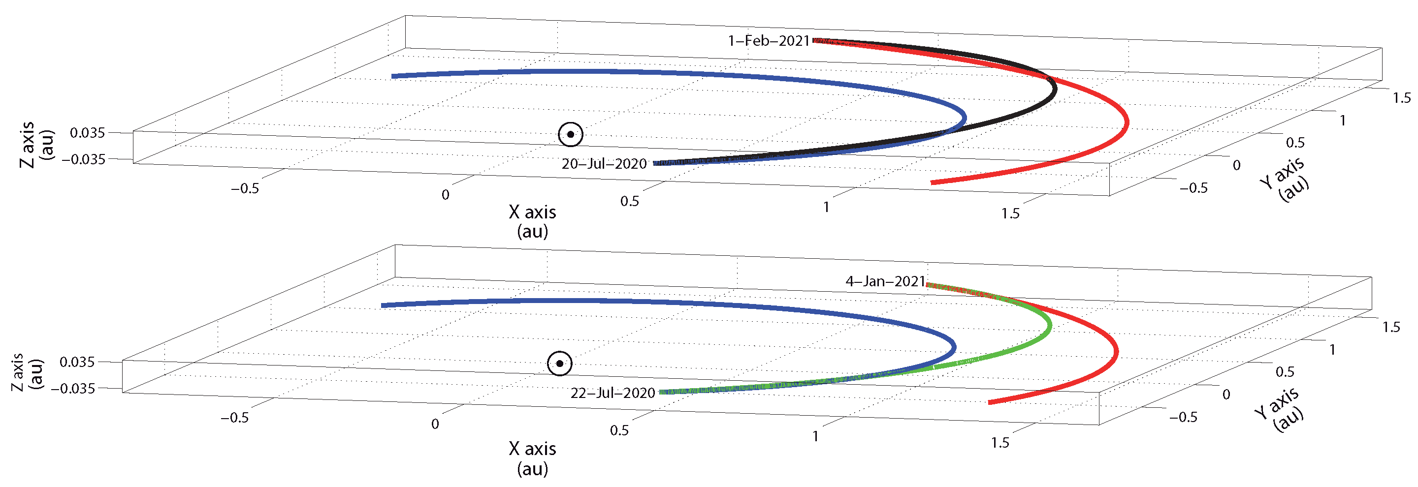
In order to analyze how a lower TOF impacts $V_{{\infty }_E}$ and $V_{{\infty }_M}$, we compare the heliocentric Earth–Mars optimal transfer orbit with the resulting orbit when a TOF 31 days less than the optimal minimum-energy trajectory is imposed. We choose a population of 500 individuals, the Stochastic Uniform function as the selection function, and the Heuristic as the crossover function. The resulting heliocentric elliptical orbits are illustrated in Figure 4, and their orbital elements are listed in

Table 2. Comparison of Earth–Mars optimal transfer heliocentric orbital parameters with respect to the mean ecliptic and equinox of J2000 for (a) the optimal launch and arrival dates in the window from 1 July 2019 to 1 November 2021 and (b) the launch and arrival dates in the window from 1 July 2019 to 1 November 2021 with the constraint of having 31 days of flight less than the optimal.

Parameter	(a)	(b)
Departure Date, $t_1$	20 July 2020 01:13:05	22 July 2020 15:20:14
Arrival Date, $t_2$	1 February 2021	4 January 2021
Arrival time	23:49:34 h	15:21:40 h
Semimajor axis, $a_{s_{\mathrm{S}}}$ (km)	198,312,598.97	202,972,264.04
Eccentricity, $e_{s_{\mathrm{S}}}$ (unitless)	0.23346	0.25130
Inclination, $i_{s_{\mathrm{S}}}$ (deg)	1.73626	0.72898
Ascending node long., ${\Omega }_{s_{\mathrm{S}}}$ (deg)	297.4399	299.8067
Arg. of the perihelium, ${\omega }_{s_{\mathrm{S}}}$ (deg)	359.6131	358.1402
True anomaly, $v_{s_{\mathrm{S}}}$ (deg)	0.4652	2.0420
$V_{{\infty }_E}$ (km/s)	3.6361	3.7803
$V_{{\infty }_M}$ (km/s)	2.7682	3.5888
Time of flight, TOF (days)	196.9420	166.0010
Total cost, C	15.9897	17.8795

. For the optimal minimum-energy orbit with a TOF of 197 days, departure on 20 July 2020 and arrival on 1 February 2021, we obtain values of $V_{{\infty }_E}=3.6361$ km/s and $V_{{\infty }_M}=2.7682$ km/s. When reducing the TOF to 166 days, departure and arrival dates change to 22 July 2020 and 4 January 2021, respectively, resulting in a more eccentric orbit, with $V_{{\infty }_M}=3.5888$ km/s significantly increased.

For the analysis henceforth, we focus on the optimal orbit for a transference in the launch window of 2026. We consider the window with the earliest launch date on 1 March 2026 and latest arrival date on 1 November 2027. We consider the same parameters for the genetic algorithms as considered in the case of the launch window of 2020: a population of 500 individuals, the Stochastic Uniform function as the selection function, and the Heuristic as crossover function. The obtained trajectory has its launch date on 31 October 2026 and arrival date on 31 August 2027.

Table 3. Elliptic heliocentric orbital elements for the optimal launch and arrival dates in the window from 1 March 2026 to 1 November 2027.

Parameter	Value
Departure Date, $t_1$	31 October 2026 05:42:13 h
Arrival Date, $t_2$	31 August 2027 16:47:12 h
Semimajor axis, $a_{s_{\mathrm{S}}}$ (km)	189,961,652.992134
Eccentricity, $e_{s_{\mathrm{S}}}$ (unitless)	0.218496
Inclination, $i_{s_{\mathrm{S}}}$ (deg)	0.8695
Periapsis argument, ${\omega }_{s_{\mathrm{S}}}$ (deg)	4.1768
Right ascension node longitude, ${\Omega }_{s_{\mathrm{S}}}$ (deg)	37.5815
True anomaly, $v_{s_{\mathrm{S}}}$ (deg)	197.9132
$V_{{\infty }_E}$ (km/s)	3.0311
$V_{{\infty }_M}$ (km/s)	2.5913
Time of flight, TOF (days)	304.4618

presents the heliocentric elliptic orbital elements for this transference. The results, particularly the higher TOF value with respect to 2020, are in good agreement with the mission analysis referenced for year 2026 in [28].

3. Determination of Earth–Mars Trajectories with Hyperbolic Orbital Objective Values

Once the launch and arrival dates for the optimal minimum-energy solution have been determined, we move on to deal with the determination of the orbit for the entry point at the Mars SOI. 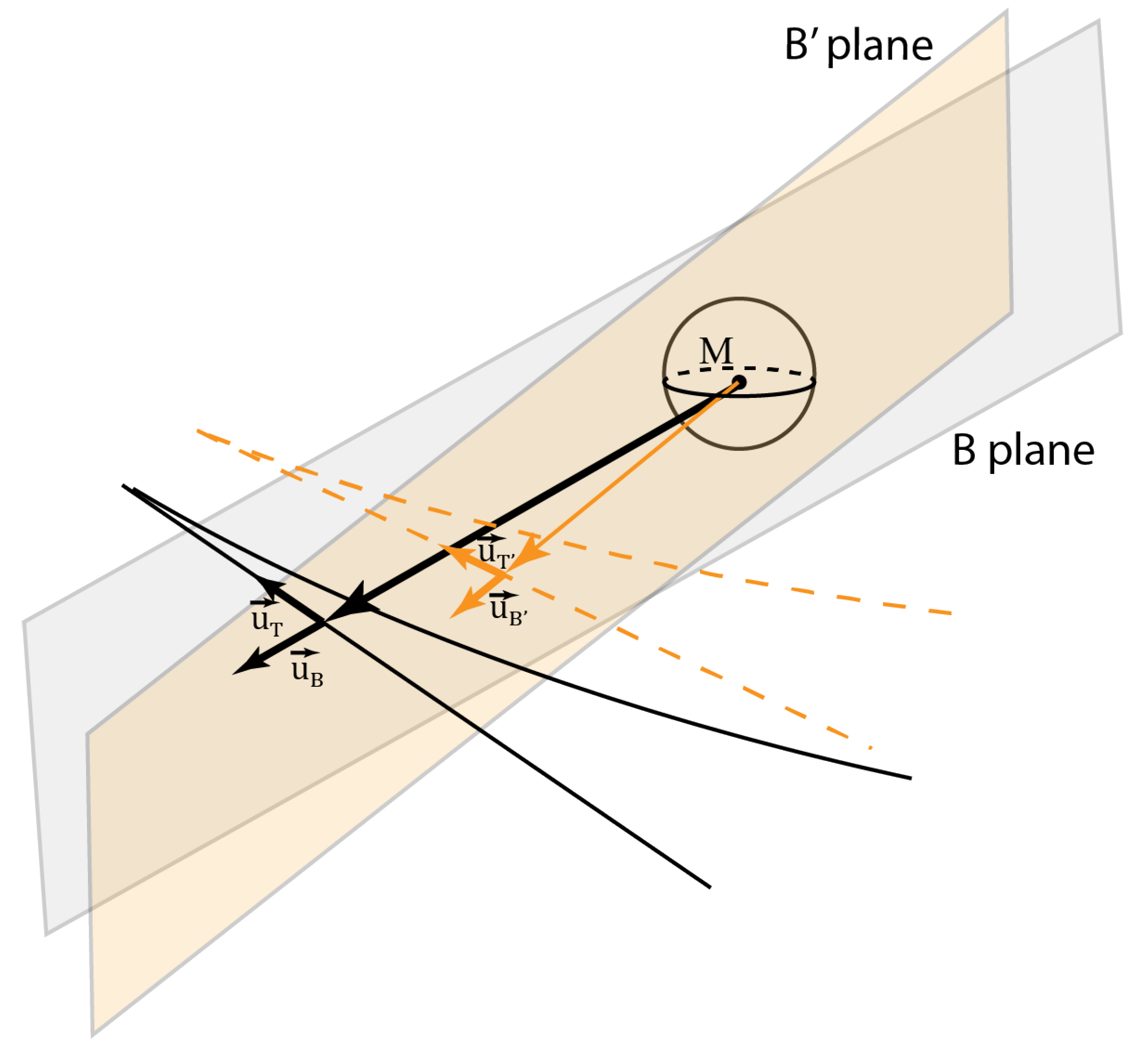To this end, we implement a procedure for matching the Earth–Mars elliptic transfer orbit and the Mars arrival hyperbolic orbit, fixing the periapsis distance, $r_{p{s}_{\mathrm{M}}}$, the arrival hyperbolic inclination, $i_{s_{\mathrm{M}}}$, and the radius for the SOI. We first present the determination of the arrival hyperbolic orbit and subsequent computation of the position and velocity at the matching point, which will be iterated with the Earth–Mars elliptic transfer afterwards. 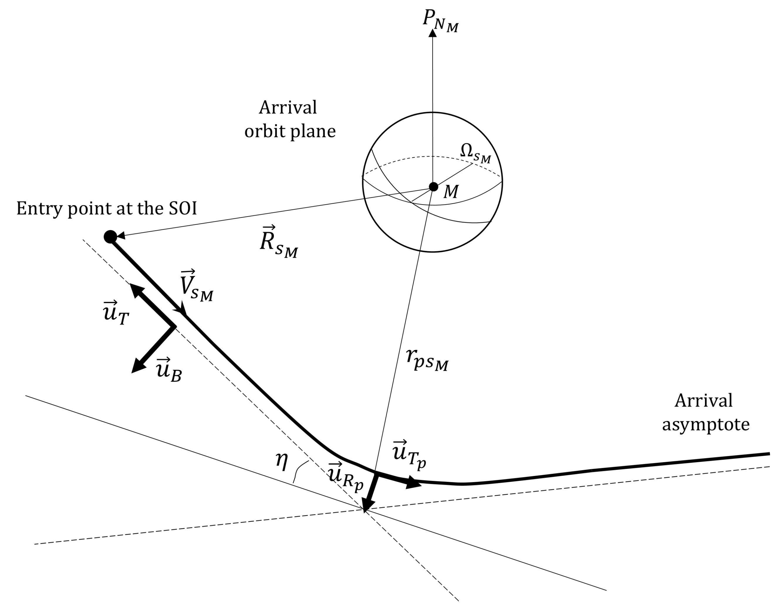The goal is to analyze the changes in the B-plane [26] due to the variations in the arrival asymptote direction.

The iterative procedure used to compute the entry point at the SOI, in which both the heliocentric elliptic transfer orbit for the obtained TOF and the areocentric hyperbolic arrival orbit match, is formulated as follows:

$${\mathbf{r}}_{s_{\mathrm{M}}}^{(i+1)}=\mathbf{g}\left(\mathbf{f}\left({\mathbf{r}}_{s_{\mathrm{M}}}^{\left(i\right)}\right)\right).$$

(7)

The function $\mathbf{f}$ provides the areocentric ecliptic transfer velocity, ${\mathbf{V}}_{{\infty }_{\mathrm{M}}}$, at the Mars SOI entry point, ${\mathbf{r}}_{s_{\mathrm{M}}}$:

$$\mathbf{f}\left({\mathbf{r}}_{s_{\mathrm{M}}}^{\left(i\right)}\right)={\mathbf{V}}_{{\infty }_{\mathrm{M}}}^{\left(i\right)},$$

(8)

obtaining first ${\mathbf{V}}_{s_{\mathrm{S}}2}$, by solving Lambert’s problem (1) with a modified condition (3),

$${\mathbf{r}}_{s_{\mathrm{S}}}\left(t_2\right)={\mathbf{r}}_{\mathrm{M}}+{\mathbf{r}}_{s_{\mathrm{M}}},$$

(9)

and then using Equation (5).

The function $\mathbf{g}$ in (7) provides the position vector, ${\mathbf{r}}_{s_{\mathrm{M}}}$, in the areocentric ecliptic reference frame:

$$\mathbf{g}\left({\mathbf{V}}_{{\infty }_{\mathrm{M}}}^{\left(i\right)}\right)={\mathbf{r}}_{s_{\mathrm{M}}}^{(i+1)}.$$

(10)

This function gathers a set of expressions to obtain ${\mathbf{r}}_{s_{\mathrm{M}}}$ at the SOI for the objective values of $i_{s_{\mathrm{M}}}$ and $r_{p{s}_{\mathrm{M}}}$, based on [22,24,25], fixing the radius of the SOI instead of the time that the spacecraft is inside the SOI, as in [22].

To this end, we first determine the areoequatorial coordinates $\left(\alpha ,\delta \right)$ of the arrival asymptote, given by $-{\mathbf{V}}_{s_{\mathrm{M}}}$ (obtained by transforming ${\mathbf{V}}_{{\infty }_{\mathrm{M}}}$ to the areocentric areoequatorial reference frame), to obtain the parameter $\sigma$ as

$$\sigma =arcsin\frac{tan\delta }{tan{i}_{s_{\mathrm{M}}}},$$

(11)

defining the minimum inclination as the value of $\parallel \delta \parallel$.

For a direct orbit, the right ascension of the ascending node, ${\Omega }_{s_{\mathrm{M}}}$, can be computed in two different ways:

$$\begin{array}{ccc}\hfill {\Omega }_{s_{\mathrm{M}}}& =& \alpha -\sigma (V_{s_{\mathrm{Mz}}}>0),\hfill \end{array}$$

(12)

$$\begin{array}{ccc}\hfill {\Omega }_{s_{\mathrm{M}}}& =& \alpha +\sigma +\pi (V_{s_{\mathrm{Mz}}}<0).\hfill \end{array}$$

(13)

The value of $V_{s_{\mathrm{M}}}$ determines the semimajor axis, $a_{s_{\mathrm{M}}}$. Then, the eccentricity of the hyperbola, $e_{s_{\mathrm{M}}}$, for a periapsis radius, $r_{p{s}_{\mathrm{M}}}$, is fixed as

$$e_{s_{\mathrm{M}}}=1+\frac{r_{p{s}_{\mathrm{M}}}}{a_{s_{\mathrm{M}}}}.$$

(14)

The true anomaly, $v_{s_{\mathrm{M}}}$, of the spacecraft at the SOI is determined using the standard procedure (i.e., [37,38]).

According to Figure 5, the unitary vectors defining the local reference system for the arrival asymptote, $\left\{{\mathbf{u}}_T,{\mathbf{u}}_B,{\mathbf{u}}_H\right\}$, are obtained as

$${\mathbf{u}}_T=\frac{-{\mathbf{V}}_{s_{\mathrm{M}}}}{\left|\right|{\mathbf{V}}_{s_{\mathrm{M}}}\left|\right|},$$

(15)

$${\mathbf{u}}_H=\left[\begin{array}{c}sin{i}_{s_{\mathrm{M}}}sin{\Omega }_{s_{\mathrm{M}}}\\ -sin{i}_{s_{\mathrm{M}}}cos{\Omega }_{s_{\mathrm{M}}}\\ cos{i}_{s_{\mathrm{M}}}\end{array}\right],$$

(16)

$${\mathbf{u}}_B={\mathbf{u}}_H\times {\mathbf{u}}_T.$$

(17)

The plane containing ${\mathbf{u}}_B$, the planet center, and perpendicular to the arrival orbit is known as the B-plane, which is considered a fundamental tool in analyzing planetary arrivals [26]. With this iterative procedure, we update the B-plane according to the objective values imposed (see Figure 6).

The vectors (15)–(17) are then transformed to a local reference system in the periapsis, $\left\{{\mathbf{u}}_{R_p},{\mathbf{u}}_{T_p},{\mathbf{u}}_H\right\}$, according to

$$\begin{array}{ccc}\hfill {\mathbf{u}}_{R_p}& =& -sin\eta {\mathbf{u}}_T+cos\eta {\mathbf{u}}_N,\hfill \end{array}$$

(18)

$$\begin{array}{ccc}\hfill {\mathbf{u}}_{T_p}& =& -cos\eta {\mathbf{u}}_T-sin\eta {\mathbf{u}}_N,\hfill \end{array}$$

(19)

where

$$\eta =arcsin\frac{1}{e_{s_{\mathrm{M}}}}.$$

(20)

Then, the areocentric areoequatorial position ${\mathbf{R}}_{s_{\mathrm{M}}}=(X_{s_{\mathrm{M}}},Y_{s_{\mathrm{M}}},Z_{s_{\mathrm{M}}})$ vector components at the SOI are determined in terms of the base vectors $\left\{{\mathbf{u}}_{R_p},{\mathbf{u}}_{T_p},{\mathbf{u}}_H\right\}$, in a classical way, as

$${\mathbf{R}}_{s_{\mathrm{M}}}=r_{s_{\mathrm{M}}}\left(cos{v}_{s_{\mathrm{M}}}{\mathbf{u}}_{R_p}+sin{v}_{s_{\mathrm{M}}}{\mathbf{u}}_{T_p}\right).$$

(21)

Finally, the position vector ${\mathbf{R}}_{s_{\mathrm{M}}}$ is transformed to obtain ${\mathbf{r}}_{s_{\mathrm{M}}}$ in the areocentric ecliptic reference frame, as a result of the function $\mathbf{g}$ in (10).

We consider that the iterative method defined by (7) converges, for a given tolerance $\tau$, when the following condition is achieved:

$$∥{\mathbf{r}}_{s_{\mathrm{M}}}^{(i+1)}-{\mathbf{r}}_{s_{\mathrm{M}}}^{\left(i\right)}∥<\tau .$$

(22)

For comparison with Table 3, in

Table 4. Elliptic heliocentric orbital elements for (a) the Earth–Mars transfer orbit at the Mars sphere of influence entry point and final hyperbolic areocentric orbital elements and (b) launch date on 31 October 2026 and arrival date on 31 August 2027, for the objective values $i_{s_{\mathrm{M}}}=i_{s_{\mathrm{M}}min}=16.{}^{\circ }1167$ and $r_{p{s}_{\mathrm{M}}}$ = 20,428 km.

Orbit	Parameter	Units	Value
(a)	Departure date, $t_1$	(UT)	31 October 2026 05:42:13 h
	Arrival date, $t_2$	(UT)	31 August 2027 16:47:12 h
	Semimajor axis, $a_{s_{\mathrm{S}}}$	(km)	189,905,238.422086
	Eccentricity, $e_{s_{\mathrm{S}}}$	(unitless)	0.218286
	Inclination, $i_{s_{\mathrm{S}}}$	(deg)	0.9311
	Periapsis argument, ${\omega }_{s_{\mathrm{S}}}$	(deg)	4.3094
	Right ascension node longitude, ${\Omega }_{s_{\mathrm{S}}}$	(deg)	37.5723
	True anomaly, $v_{s_{\mathrm{S}}}$	(deg)	197.9302
	$V_{{\infty }_{\mathrm{E}}}$	(km/s)	3.0333
	$V_{{\infty }_{\mathrm{M}}}$	(km/s)	2.5763
	Time of flight, TOF	(days)	304.4618
(b)	Semimajor axis, $a_{s_{\mathrm{M}}}$	(km)	6600.229103
	Eccentricity, $e_{s_{\mathrm{M}}}$	(unitless)	4.0950441
	Inclination, $i_{s_{\mathrm{M}}}$	(deg)	16.1167
	Periapsis argument, ${\omega }_{s_{\mathrm{M}}}$	(deg)	194.1344
	Right ascension node longitude, ${\Omega }_{s_{\mathrm{M}}}$	(deg)	162.7116
	True anomaly at $t_2$, $v_{s_{\mathrm{M}}}$	(deg)	258.4533
	Periapsis radius, $r_{p{s}_{\mathrm{M}}}$	(km)	20,467.9232
	Arrival at periapsis date, $t_p$	(UT)	31 August 2027 20:03:55

, we present the results for the elliptic transfer orbit in the heliocentric ecliptic reference frame for the minimum-energy TOF ($304.4618$ days), the minimum arrival hyperbolic inclination ($i_{s_{\mathrm{M}}min}={16}^{\circ }.1167$), $r_{p{s}_{\mathrm{M}}}$ = 20,428 km, and a SOI of $r_{I_{\mathrm{M}}}$ = 577,239 km. We note that $V_{{\infty }_{\mathrm{M}}}$ changes by $0.015$ km/s approximately. Also, the resulting areocentric hyperbolic arrival trajectory orbital elements in the areoequatorial reference frame are shown in Table 4.

4. Mars Arrival Maneuvers Evaluation for an Areostationary Mission

We now conduct a preliminary evaluation of the total impulsive maneuvers $\Delta V_M$ needed to capture the probe and to place it in an areostationary orbit:

$$\Delta V_M=\Delta V_c+\Delta V_P+\Delta V_A+\Delta V_i,$$

(23)

where $\Delta V_c$ is the capture maneuver to avoid the probe leaving the SOI on a flyby trajectory; $\Delta V_P$ and $\Delta V_A$ are the two Hohmann transfer maneuvers, at the perigee and apogee, respectively, designed to obtain a transfer orbit from the capture orbit to the target areostationary orbit; and $\Delta V_i$ is the inclination correction maneuver to reach the final zero desired inclination.

If we consider a $\Delta V_c$ maneuver at the periapsis of the hyperbolic orbit in order to obtain a circular capture orbit, its magnitude would be

$$\Delta V_c=\sqrt{V_{{\infty }_{\mathrm{M}}}^2+2\frac{{\mu }_M}{r_{p{s}_{\mathrm{M}}}}}-\sqrt{\frac{{\mu }_M}{r_{p{s}_{\mathrm{M}}}}}.$$

(24)

The hyperbolic periapsis distance, $r_{p{s}_{\mathrm{M}}}$, is calculated as follows:

$$\begin{array}{ccc}{r}_{p{s}_{\mathrm{M}}}& =& a_{s_{\mathrm{M}}}(e_{s_{\mathrm{M}}}-1),\end{array}$$

(25)

with $a_{s_{\mathrm{M}}}$ as the hyperbolic semimajor axis and $e_{s_{\mathrm{M}}}$ as the hyperbolic eccentricity.

The two Hohmann transfer maneuvers required to achieve an orbit at the areostationary semimajor axis, $r_A=$ 20,428 km, in the case that $r_{p{s}_{\mathrm{M}}}<r_A$, are calculated as

$$\begin{array}{ccc}\Delta V_P& =& \sqrt{\frac{{\mu }_M}{r_{p{s}_{\mathrm{M}}}}}\left(\sqrt{\frac{2r_A}{r_{p{s}_{\mathrm{M}}}+r_A}}-1\right),\end{array}$$

(26)

$$\begin{array}{ccc}\Delta V_A& =& \sqrt{\frac{{\mu }_M}{r_A}}\left(1-\sqrt{\frac{2r_{p{s}_{\mathrm{M}}}}{r_{p{s}_{\mathrm{M}}}+r_A}}\right).\end{array}$$

(27)

Finally, the inclination maneuver is performed at the stationary distance in order to minimize its magnitude. For a maneuver at the node, this is obtained as

$$\Delta V_i=\sqrt{2\frac{{\mu }_M}{r_A}-2\frac{{\mu }_M}{r_A}cos{i}_{s_{\mathrm{M}}}},$$

(28)

where $i_{s_{\mathrm{M}}}$ is the hyperbolic inclination.

In the case that $r_{p{s}_{\mathrm{M}}}>r_A$, the inclination maneuver at the node would be the first to be performed at the $r_{p{s}_{\mathrm{M}}}$ distance:

$$\Delta V_i=\sqrt{2\frac{{\mu }_M}{r_{p{s}_{\mathrm{M}}}}-2\frac{{\mu }_M}{r_{p{s}_{\mathrm{M}}}}cos{i}_{s_{\mathrm{M}}}}.$$

(29)

Then, the two Hohmann maneuvers would be performed according to the following equations:

$$\begin{array}{ccc}\Delta V_P& =& \sqrt{\frac{{\mu }_M}{r_{p{s}_{\mathrm{M}}}}}\left(1-\sqrt{\frac{2r_A}{r_{p{s}_{\mathrm{M}}}+r_A}}\right),\end{array}$$

(30)

$$\begin{array}{ccc}\Delta V_A& =& \sqrt{\frac{{\mu }_M}{r_A}}\left(\sqrt{\frac{2r_{p{s}_{\mathrm{M}}}}{r_{p{s}_{\mathrm{M}}}+r_A}}-1\right).\end{array}$$

(31)

As can be seen from Equations (24) to (31), the periapsis distance, $r_{p{s}_{\mathrm{M}}}$, and the orbital inclination of the arrival trajectory with respect to Mars, $i_{s_{\mathrm{M}}}$, are the key design parameters in order to minimize the required impulses. Corrections to change the approach asymptotic plane are not considered, and neither are the combinations of the capture maneuver with the first Hohmann maneuver or the inclination maneuver with the second Hohmann maneuver.

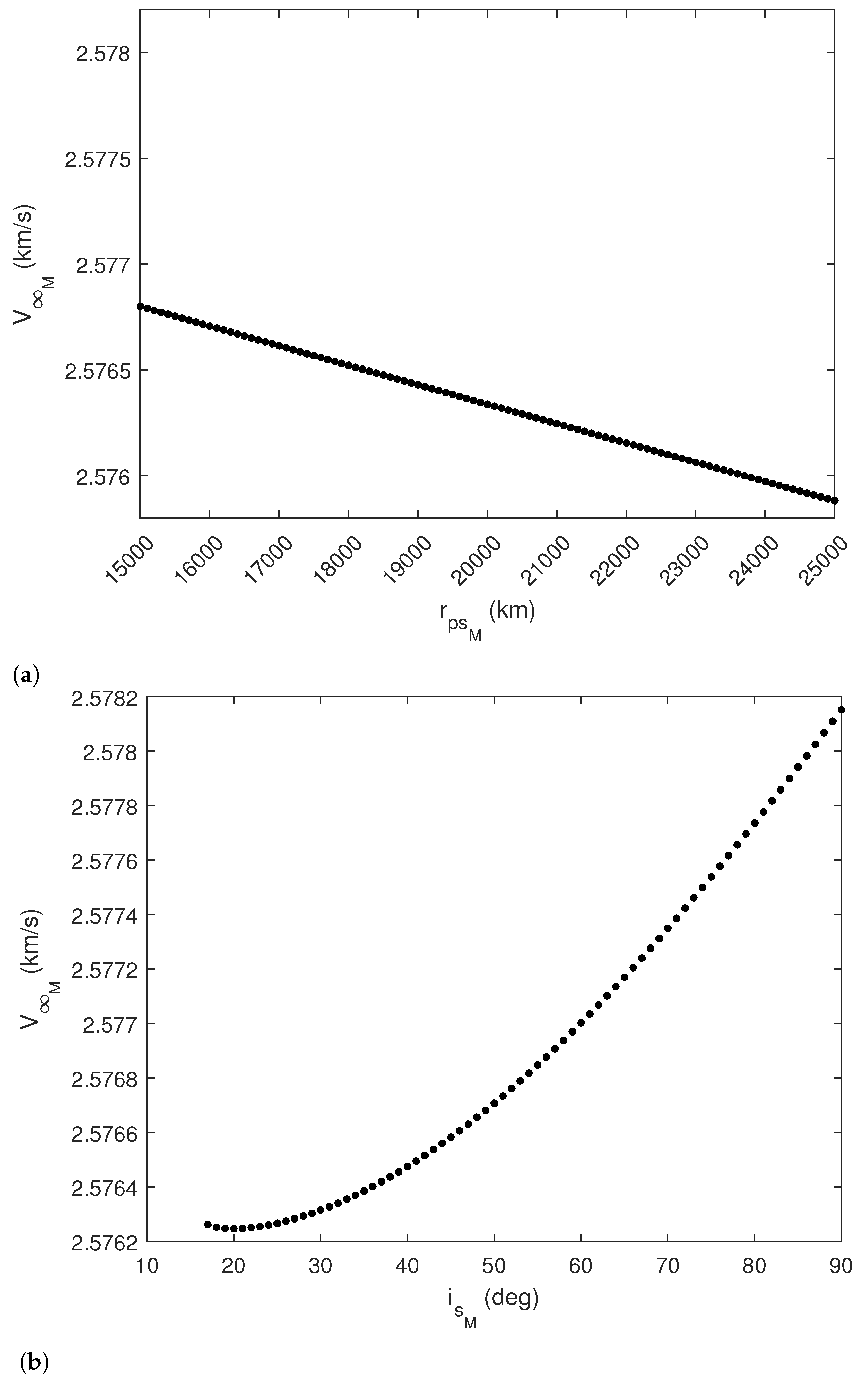
Several numerical simulations are carried out to analyze the magnitude of these impulses due to the variations in the B-plane when different imposed values for TOF, $i_{s_{\mathrm{M}}}$, and $r_{p{s}_{\mathrm{M}}}$ are considered.

We fix the launch window for 2026 according to the parameters given in Table 3 for the launch and arrival dates connecting Earth and Mars that minimize $V_{{\infty }_{\mathrm{M}}}$. In the first set of simulations, we consider different imposed objective values for the inclination, $i_{s_{\mathrm{M}}}$, and the periapsis radius, $r_{p{s}_{\mathrm{M}}}$, to determine the entry point at the SOI, using the iterative procedure defined in (7) to evaluate the total impulse $\Delta V_M$ in Equation (23). We consider different values for $i_{s_{\mathrm{M}}}$, ranging in the interval $\left[i_{s_{\mathrm{M}}min},{90}^{\circ }\right)$, and for $r_{p{s}_{\mathrm{M}}}$, in the interval $\left[15,000\mathrm{km},25,000\mathrm{km}\right]$, with the arrival velocity, $V_{{\infty }_{\mathrm{M}}}$, recalculated for the different entry points.

Figure 7a,b represent the results obtained for $V_{{\infty }_{\mathrm{M}}}$ with different values of $r_{p{s}_{\mathrm{M}}}$ and $i_{s_{\mathrm{M}}}$, respectively. For the objective conditions of $i_{s_{\mathrm{M}}}={16}^{\circ }.1167$, which corresponds to the $i_{s_{\mathrm{M}}min}$ for $r_{p{s}_{\mathrm{M}}}=r_A=$ 20,428 km, a value of $V_{{\infty }_{\mathrm{M}}}=2.5763$ km/s is obtained. As can be observed in Figure 7a for $i_{s_{\mathrm{M}}min}$, $V_{{\infty }_{\mathrm{M}}}$ decreases linearly when increasing $r_{p{s}_{\mathrm{M}}}$ from $2.5768$ km/s to $2.5759$ km/s. Figure 7b shows variations of about $2\times {10}^{-3}$ km/s in $V_{{\infty }_{\mathrm{M}}}$, for the areostationary distance, as the objective inclination increases from $i_{s_{\mathrm{M}}min}$ to ${90}^{\circ }$.

Table 5. Interplanetary transfer energy variations for the considered combinations of $i_{s_{\mathrm{M}}}$ and the maximum and minimum $r_{p{s}_{\mathrm{M}}}$ and of $r_{p{s}_{\mathrm{M}}}=r_A$ with the maximum and minimum $i_{s_{\mathrm{M}}}$.

${\mathit{i}}_{{\mathit{s}}_{\mathbf{M}}}$ (deg)	${\mathit{r}}_{{\mathit{ps}}_{\mathbf{M}}}$ (km)	${\mathit{C}}_3$ (${\mathbf{km}}^2/{\mathbf{s}}^2$)	${\mathit{V}}_{{\mathit{\infty }}_{\mathit{M}}}$ (km/s)	C
$i_{s_{\mathrm{M}}min}=16.1158$	15,000	9.2014	2.5768	11.7782
$i_{s_{\mathrm{M}}min}=16.1175$	25,000	9.2008	2.5759	11.7767
$i_{s_{\mathrm{M}}min}=16.1167$	$r_A=20,428$	9.2011	2.5763	11.7774
90	$r_A=20,428$	9.2123	2.5781	11.7904

summarizes the values for the $C_3$, $V_{{\infty }_{\mathrm{M}}}$, and total cost C of Equation (6) for the minimum and maximum values of $r_{p{s}_{\mathrm{M}}}$ and $i_{s_{\mathrm{M}}}$ considered.

Figure 8a,b represent the values of $\Delta V_c$, $\Delta V_i$, $\Delta V_A$, $\Delta V_P$, and the total $\Delta V_{\mathrm{M}}$ for different values of $r_{p{s}_{\mathrm{M}}}$ and $i_{s_{\mathrm{M}}}$ to achieve the circular areostationary orbit at $r_A$ with zero areoequatorial inclination. In the case that $r_{p{s}_{\mathrm{M}}}<r_A$, the maneuvers are computed using (24) and (26)–(28). In the other case, the maneuvers are computed by means of (24) and (29)–(31).

As can be seen in Figure 8a, with the above-described strategy, the values for the capture maneuver $\Delta V_c$ change, for $i_{s_{\mathrm{M}}min}$, from $1.8246$ km/s for $r_{p{s}_{\mathrm{M}}}$ = 15,000 km to $1.8631$ km/s for $r_{p{s}_{\mathrm{M}}}$ = 25,000 km, depending on the different objective periapsis radius considered. Obviously, the Hohmann maneuver vanishes for a capture at $r_A$, and its value varies from $0.2404$ km/s for $r_{p{s}_{\mathrm{M}}}$ = 15,000 km to $0.1387$ km/s for $r_{p{s}_{\mathrm{M}}}$ = 25,000. The inclination maneuver, $\Delta V_i$, to achieve zero inclination, from the $i_{s_{\mathrm{M}}min}$ for each $r_{p{s}_{\mathrm{M}}}$, has a slight variation from 0.4062 km/s to 0.3673 km/s. The minimum for the total amount, $\Delta V_M$, has a value of $2.2493$ km/s, which corresponds to $r_{p{s}_{\mathrm{M}}}=r_A$. This magnitude rises to $2.4712$ km/s for $r_{p{s}_{\mathrm{M}}}$ = 15,000 km and to $2.3691$ km/s for $r_{p{s}_{\mathrm{M}}}$ = 25,000 km.

Figure 8b shows that, for $r_{p{s}_{\mathrm{M}}}=r_A$, with $\Delta V_H=0$ km/s, $\Delta V_M$ increases when different values for the objective hyperbolic inclination are considered. From the same minimum of $\Delta V_M=2.2493$ km/s for $i_{s_{\mathrm{M}}min}=16.{}^{\circ }1167$, the total quantity of impulses rises to $3.8922$ km/s, as illustrated in Figure 8a.

In a second set of simulations, we consider a different strategy to evaluate the Oberth effect that, due to the potential energy for a capture near the Mars surface, allows one to reduce the required $\Delta V_M$. To this end, we consider a capture into an elliptical trajectory with a low periapsis radius and an apoapsis at the stationary orbit. Then, a circularization process is performed at the apoapsis. For a capture at a periapsis of $r_{p{s}_{\mathrm{M}}}=r_M+300$ km into an ellipse with an apoapsis of $r_A$, the value of the impulse required to obtain a circular orbit at the areostationary distance is decreased to $1.6764$ km/s, with $\Delta V_c=1.0294$ km/s and $\Delta V_A=0.6470$ km/s. The total $\Delta V_M=2.0834$ km/s reduces $0.1659$ km/s with respect to the previous strategy.

Finally, we analyze the influence of the TOF in $\Delta V_{\mathrm{M}}$ for a possible launch date delay. We consider up to two weeks delay from 31 October 2026 for the launch date and up to two months after 31 August 2027 for the arrival date for the minimum $i_{s_{\mathrm{M}}}$. In the first case, a capture into a circular orbit of $r_{p{s}_{\mathrm{M}}}=r_A$ is considered, as shown in Figure 9a. In the second case, a capture into an ellipse with $r_{p{s}_{\mathrm{M}}}=r_M+300$ and an apoapsis of $r_A$ is considered, as shown in Figure 9b. It can be noticed, by comparing Figure 9a,b, that the second case is less sensitive to TOF variations. For case (a), a delay of 14 days at departure and 60 at arrival, increases the value of $2.25$ km/s by $0.75$ km/s, corresponding to the minimum-energy transfer TOF of 304 days, instead of an increase of $0.52$ km/s from the value $2.08$ km/s in case (b). In both cases, a launch delay of 14 days maintaining a TOF of 304 days would increase $\Delta V_M$ by 0.25 km/s.

5. Conclusions

In this paper, we conducted a preliminary analysis of the impulsive maneuvers cost to transfer a spacecraft from Earth to Mars and to position it in an areostationary orbit. We first obtained the minimum-energy interplanetary transfer from Earth to Mars by applying genetic algorithms to select launch and arrival dates. Several simulations were carried out to analyze the performance of the genetic algorithms. Results show that differences in the final energy cost and the time of flight are negligible, and the only significant change is the CPU time needed to converge, which is dependent on the population size.

With the optimized launch and arrival dates, an iterative procedure was used to match the interplanetary trajectory obtained with the genetic algorithms, with an entry hyperbola defined by imposing objective conditions for the inclination and the periapsis radius of the orbit. Two different strategies were computed to evaluate the cost of the mission, $\Delta V_M$: The first includes a capture maneuver to a circular orbit at different periapsis radii, as well as Hohmann maneuvers and an inclination maneuver; The second includes a capture maneuver to an elliptic orbit with a low periapsis and an apoapsis at the areostationary orbit. Simulations with different imposed conditions on the entry hyperbola were conducted depending on the two key parameters: the hyperbolic inclination, $i_{s_{\mathrm{M}}}$, and the periapsis radius, $r_{p{s}_{\mathrm{M}}}$. For a circular capture at the stationary radius, results show that for a 2026 mission with a TOF of 304 days for the minimum-energy Earth–Mars transfer trajectory, the values achieved are $\Delta V_c=1.84$, $\Delta V_H=0$ and $\Delta V_i=0.41$, being the total impulse $\Delta V_M=2.25$ km/s for the minimum possible inclination $i_{s_{\mathrm{M}}}=16.{}^{\circ }1167$ and $r_{p{s}_{\mathrm{M}}}$ = 20,428 km corresponding to an areostationary radius. For an elliptical capture with a periapsis of $r_{p{s}_{\mathrm{M}}}=r_M+300$ km and an apoapsis of 20,428, the values achieved are $\Delta V_c=1.03$, $\Delta V_A=0.65$, and $\Delta V_i=0.41$, the total impulse amounting to $\Delta V_M=2.08$ km/s. A launch delay of two weeks would increase this minimum value of $\Delta V_M$ by 0.25 km/s in both cases. The capture into an ellipse with a delay of 14 days at departure and 60 at arrival is less sensitive to TOF variations, increasing the total $\Delta V_M$ by $0.52$ km/s, instead of $0.75$ for the direct circular capture.