
Comparative Study of Metaheuristic Optimization of Convolutional Neural Networks Applied to Face Mask Classification


Abstract
:1. Introduction
2. Background
3. Intelligence Techniques
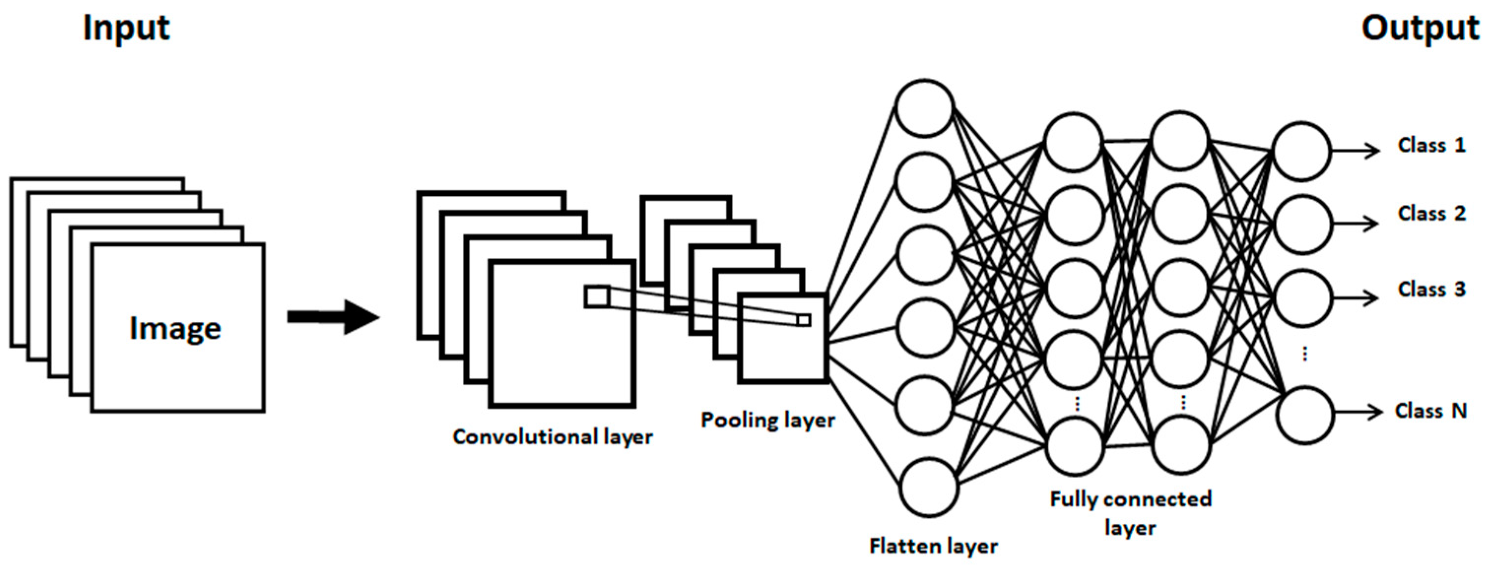
3.1. Convolutional Neural Networks
3.2. Nature-Inspired Algorithms
3.2.1. Particle Swarm Optimization
3.2.2. Grey Wolf Optimizer
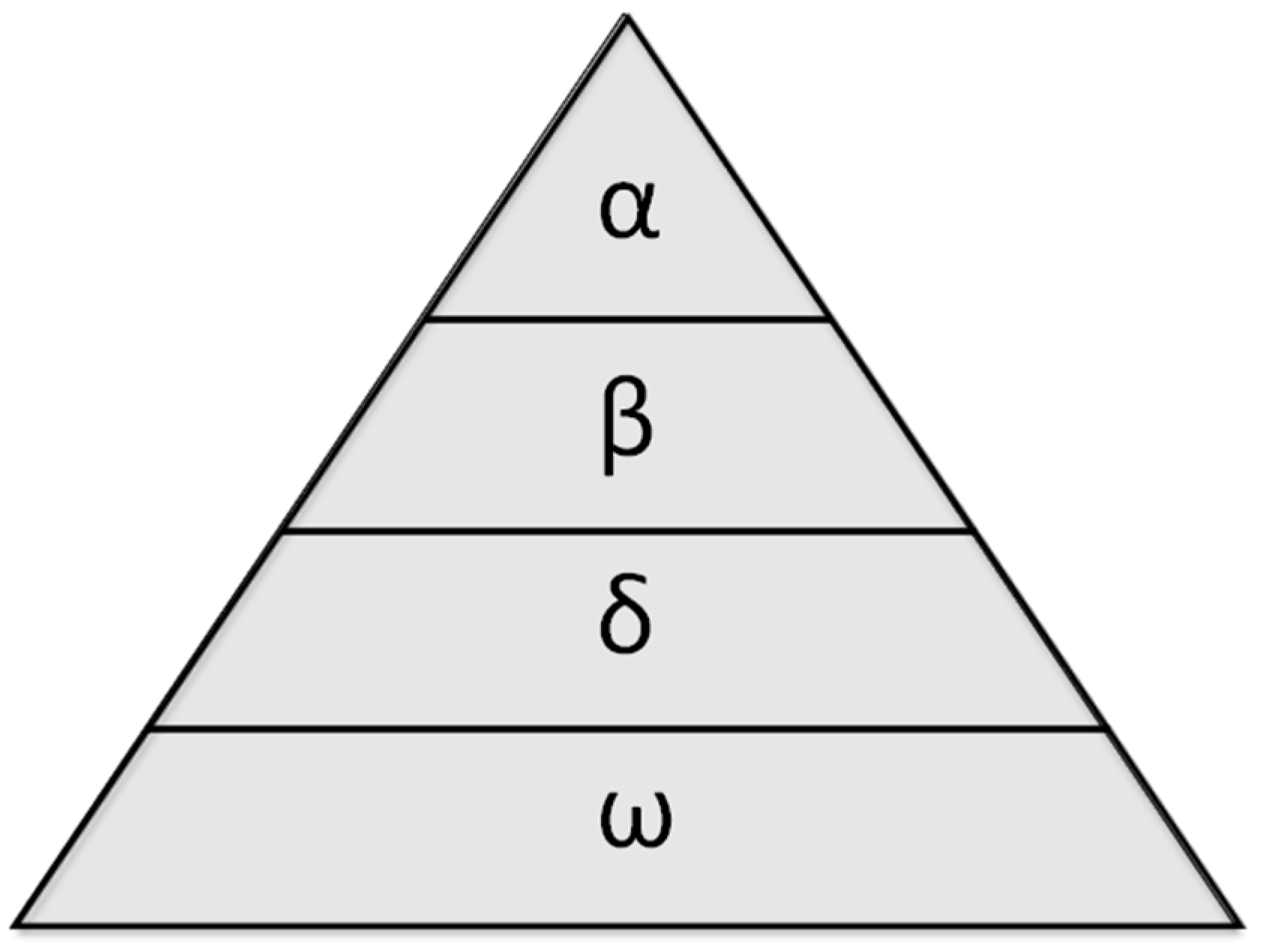
- Social hierarchy: The three best solutions are alpha (α), beta (β), and delta (δ). The wolves belonging to the lowest level are the omegas (ω).
- Encircling prey: The process of prey encircling during hunting are represented by Equations (4) and (5).
- Hunting: The first three levels in the dominant hierarchy know the prey position. With their positions, the wolves belonging to the lowest level (omega) can update their position using Equations (9)–(11).
- Attacking prey: The process is also known as exploitation, where the current position of an agent and the prey allows it to establish the next position of the agent. This position is calculated using and vector with random values in an interval [−2].
- Search for prey: The process is also known as exploration, where vector is used with values in [0, 2] to provide diversity to the population and avoid local optimal.
3.2.3. Whale Optimization Algorithm
- Encircling prey: The whales encircle the prey because they know its position. The whale closest to the prey becomes the best solution. Equations (3) and (4) allow the update of the position of the rest of the agents.
- Bubble-net attacking method: This process is also known as exploitation and is very similar to the one in the GWO, where the distance between the agent and the prey is determined. The process can be accomplished using two approaches:
- Mechanism of shrinking encircling: In Equation (5), the values of decrease every iteration, and an interval ] is used to generate random values for the vector .
- Spiral updating position: The helix-shaped movement of whales between the whale and prey position is mimicked by Equation (12).
- Search for prey: This process is also known as exploration, where the whales seek randomly based on the position of others. To force the exploration, the vector has numbers less than −1 and greater than 1. The process is defined by Equations (13) and (14).
3.2.4. Bat Algorithm
- Echolocation is used for all the bats to sense distance, and they know the difference between the prey and other kind of elements.
- To search for prey, each bat flies randomly in a position with a velocity . This task is performed by changing loudness A and wavelength . Depending on the closeness of its objective, the bat regulates the wavelength of its emitted pulses and regulate the rate of pulse emission .
- The loudness is assumed to be a large value positive number to a minimum constant value .
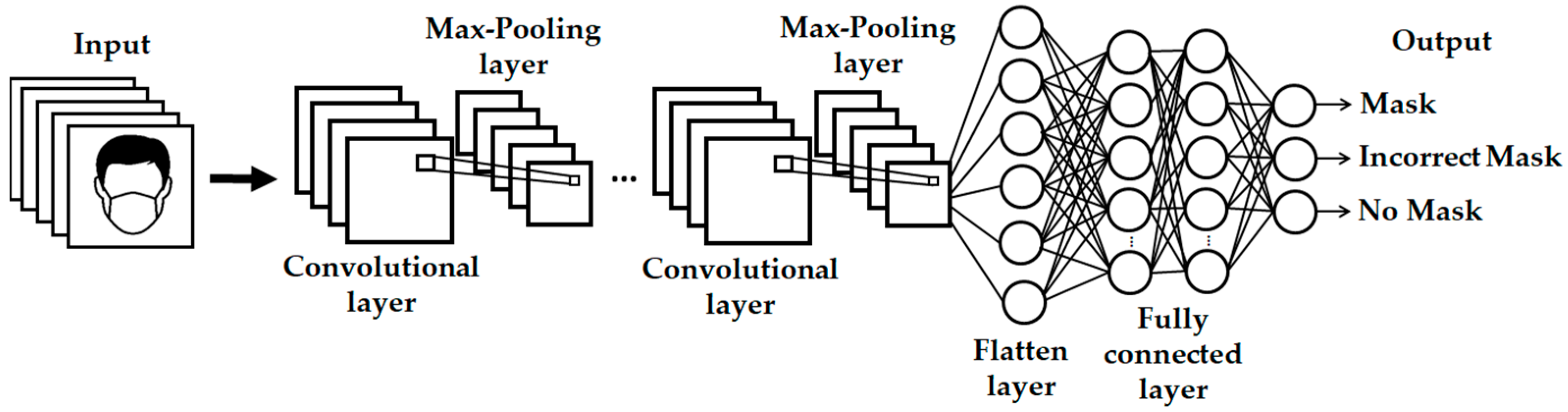
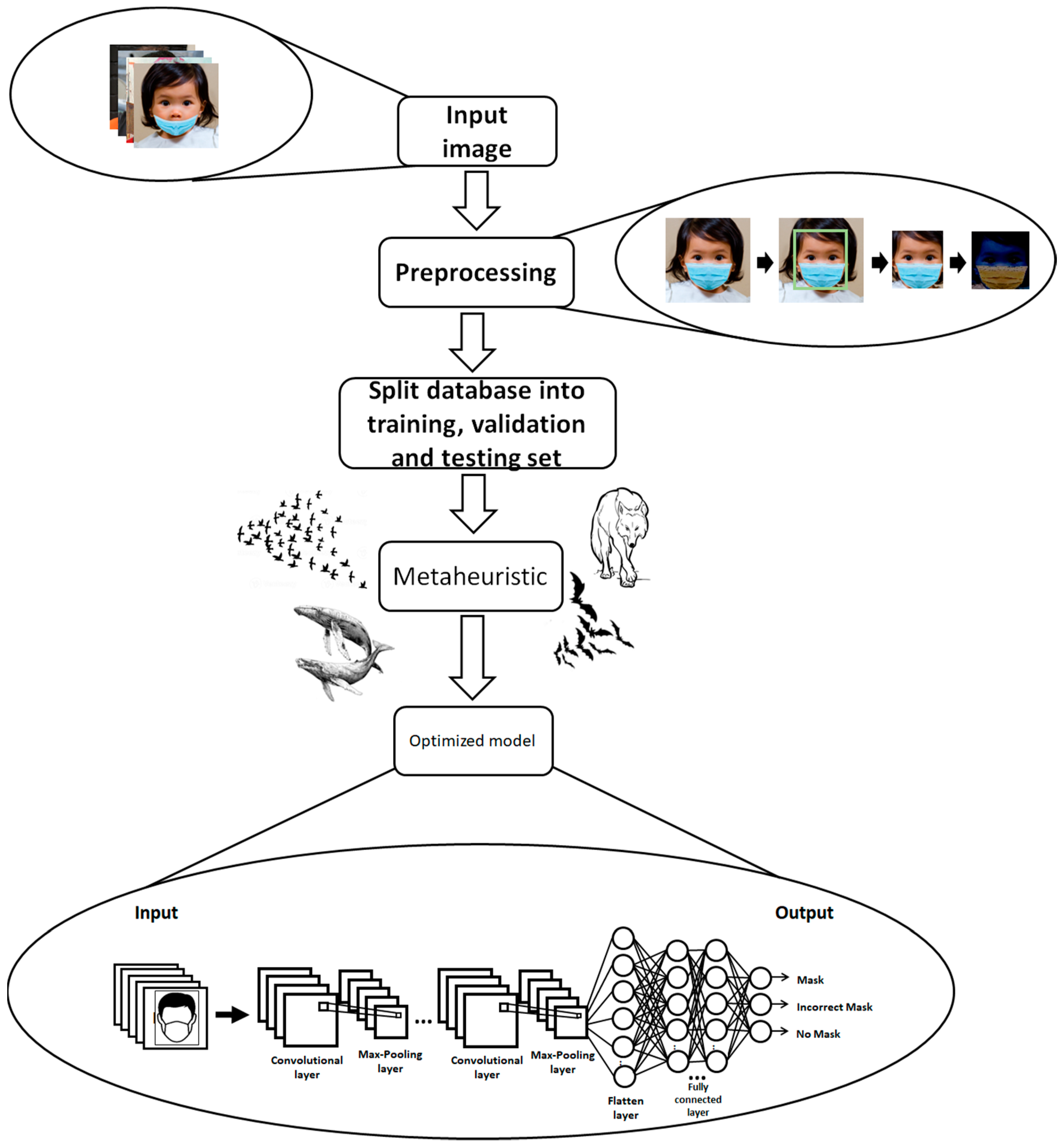
4. Proposed Method
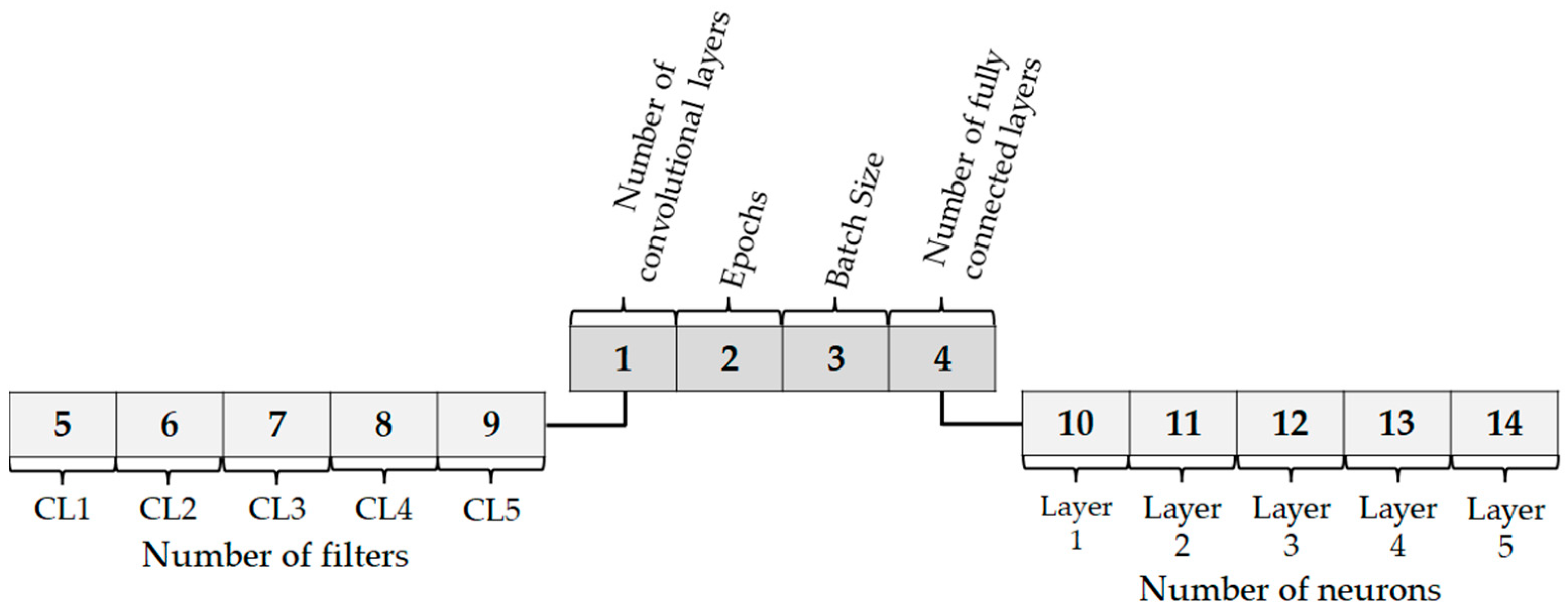
4.1. Description of the Optimization
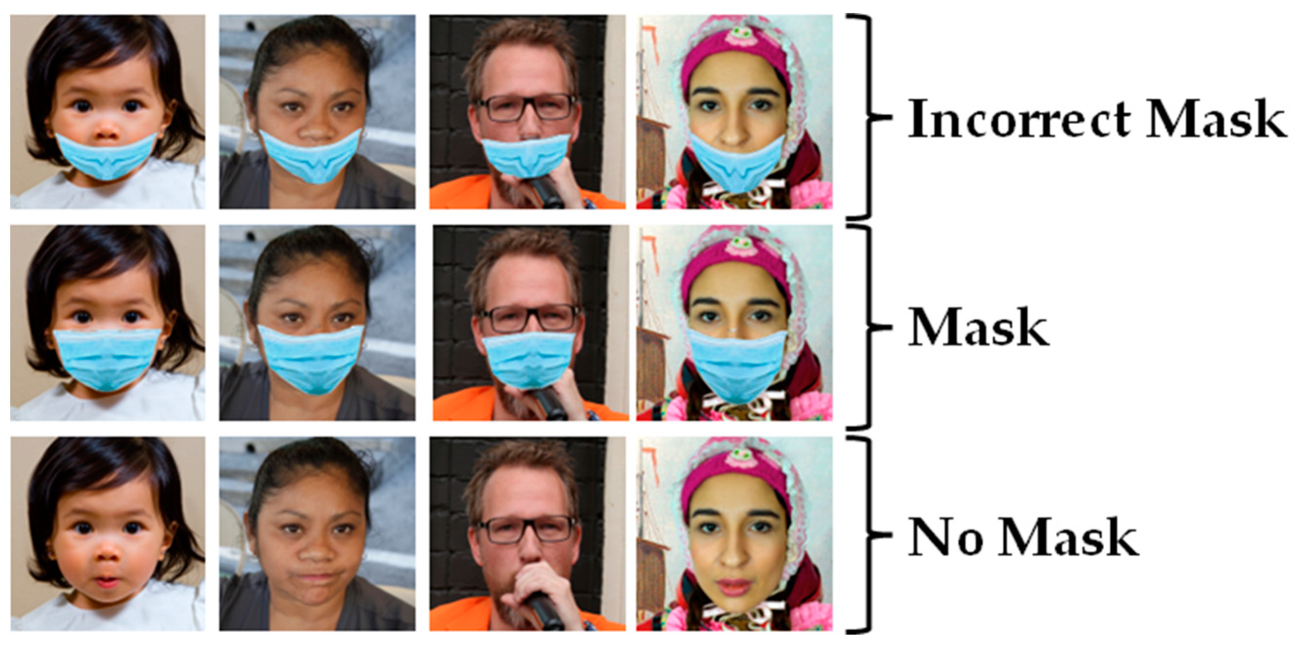
4.2. Database
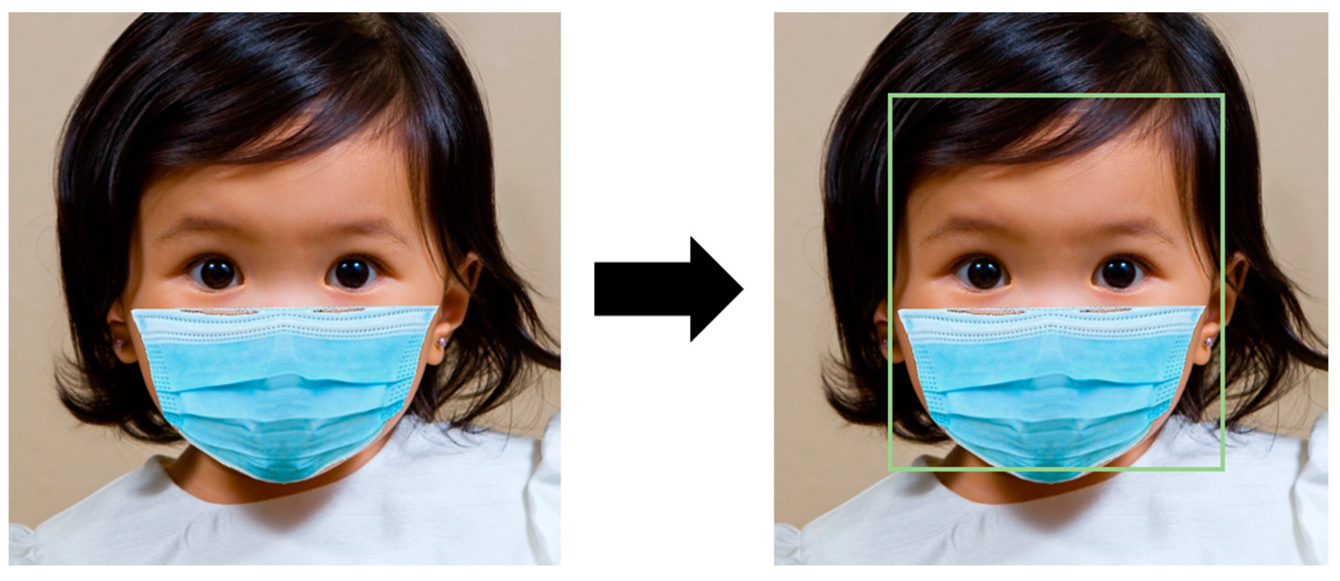
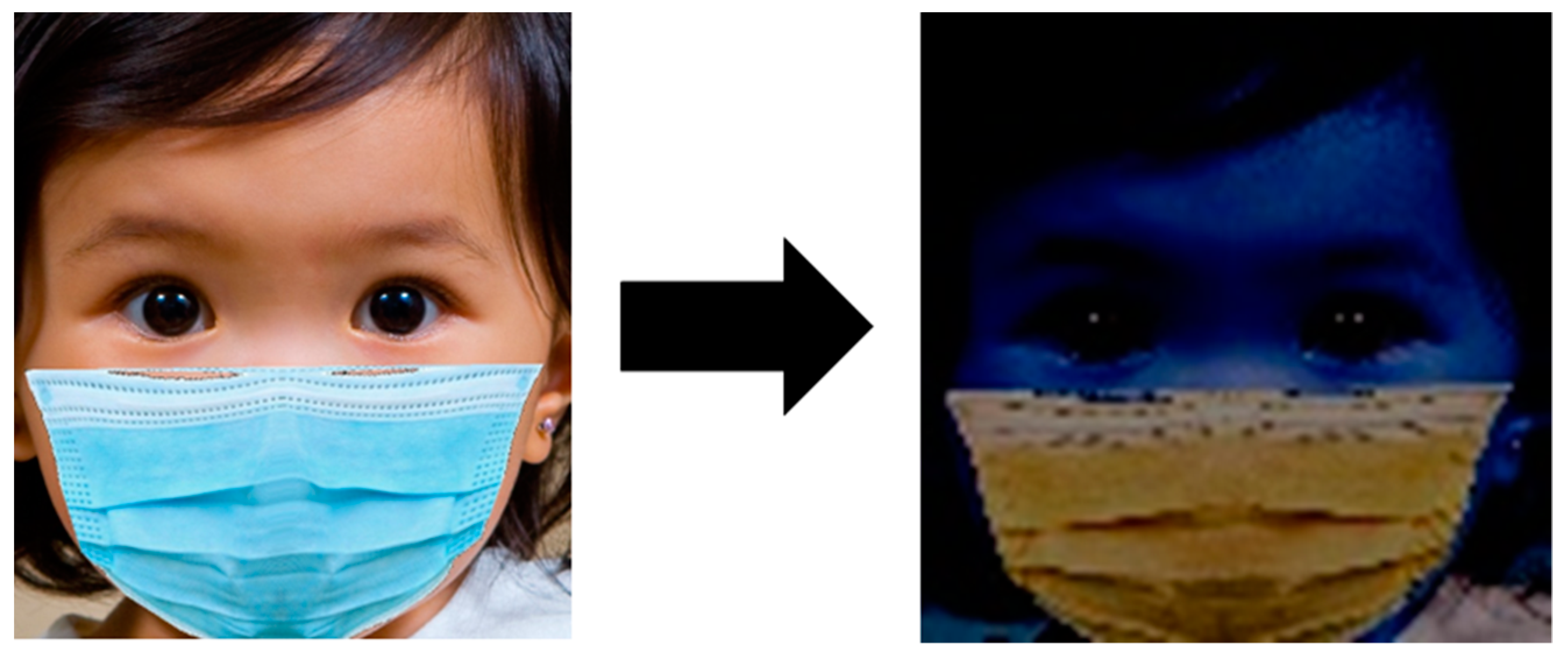
4.3. Preprocessing
5. Experimental Results
5.1. PSO Results
5.2. WOA Results
5.3. BA Results
5.4. GWO Results
5.5. Comparison of Results
6. Statistical Comparison
7. Conclusions
Author Contributions
Funding
Data Availability Statement
Acknowledgments
Conflicts of Interest
References
- Eikenberry, S.; Mancuso, M.; Iboi, E.; Phan, T.; Eikenberry, K.; Kuang, Y.; Kostelich, E.; Gumel, A. To mask or not to mask: Modeling the potential for face mask use by the general public to curtail the COVID-19 pandemic. Infect. Dis. Model. 2020, 5, 293–308. [Google Scholar] [CrossRef] [PubMed]
- Garcia Godoy, L.; Jones, A.; Anderson, T.; Fisher, C.; Seeley, K.; Beeson, E.; Zane, H.; Peterson, J.; Sullivan, P. Facial protection for healthcare workers during pandemics: A scoping review. BMJ Glob. Health 2020, 5, e002553. [Google Scholar] [CrossRef] [PubMed]
- MacIntyre, C.; Cauchemez, S.; Dwyer, D.; Seale, H.; Cheung, P.; Browne, G.; Fasher, M.; Wood, J.; Gao, Z.; Booy, R.; et al. Face Mask Use and Control of Respiratory Virus Transmission in Households. Emerg. Infect. Dis. 2009, 15, 233–241. [Google Scholar] [CrossRef] [PubMed]
- MacIntyre, C.; Chughtai, A.; Rahman, B.; Peng, Y.; Zhang, Y.; Seale, H.; Wang, X.; Wang, Q. The efficacy of medical masks and respirators against respiratory infection in healthcare workers. Influenza Other Respir. Viruses 2017, 11, 511–517. [Google Scholar] [CrossRef] [PubMed]
- Pham-Hoang-Nam, A.; Le-Thi-Tuong, V.; Phung-Khanh, L.; Ly-Tu, N. Densely Populated Regions Face Masks Localization and Classification Using Deep Learning Models. In Proceedings of the Sixth International Conference on Research in Intelligent and Computing, Thủ Dầu Một, Vietnam, 3–4 June 2021. [Google Scholar]
- Sethi, S.; Kathuria, M.; Kaushik, T. Face mask detection using deep learning: An approach to reduce risk of Coronavirus spread. J. Biomed. Inform. 2021, 120, 103848. [Google Scholar] [CrossRef]
- Yu, J.; Zhang, W. Face Mask Wearing Detection Algorithm Based on Improved YOLO-v4. Sensors 2021, 21, 3263. [Google Scholar] [CrossRef]
- Mar-Cupido, R.; Garcia, V.; Rivera, G.; Sánchez, J. Deep transfer learning for the recognition of types of face masks as a core measure to prevent the transmission of COVID-19. Appl. Soft Comput. 2022, 125, 109207. [Google Scholar] [CrossRef]
- Umer, M.; Sadiq, S.; Alhebshi, R.; Alsubai, S.; Hejaili, A.; Eshmawi, A.; Nappi, M.; Ashraf, I. Face mask detection using deep convolutional neural network and multi-stage image processing. Image Vis. Comput. 2023, 133, 104657. [Google Scholar] [CrossRef]
- Ramakrishnan, K.; Balakrishnan, V.; Wong, H.; Tay, S.; Soo, K.; Kiew, W. Face Mask Wearing Classification Using Machine Learning. Eng. Proc. 2023, 41, 13. [Google Scholar]
- Habib, S.; Alsanea, M.; Aloraini, M.; Al-Rawashdeh, H.; Islam, M.; Khan, S. An Efficient and Effective Deep Learning-Based Model for Real-Time Face Mask Detection. Sensors 2022, 22, 2602. [Google Scholar] [CrossRef]
- Wakchaure, A.; Kanawade, P.; Jawale, M.; William, P.; Pawar, A. Face Mask Detection in Realtime Environment using Machine Learning based Google Cloud. In Proceedings of the International Conference on Applied Artificial Intelligence and Computing, Salem, India, 9–11 May 2022. [Google Scholar]
- Mirjalili, S. Evolutionary Algorithms and Neural Networks: Theory and Applications, 1st ed.; Springer: London, UK, 2019. [Google Scholar]
- Du, K.; Swamy, M. Search and Optimization by Metaheuristics: Techniques and Algorithms Inspired by Nature, 1st ed.; Birkhäuser Cham: Berlín, Germany, 2018. [Google Scholar]
- Hassanien, A.; Emary, E. Swarm Intelligence: Principles, Advances and Applications, 1st ed.; CRC Press: Boca Raton, FL, USA, 2015. [Google Scholar]
- Iba, H. AI and SWARM: Evolutionary Approach to Emergent Intelligence, 1st ed.; CRC Press: Boca Raton, FL, USA, 2019. [Google Scholar]
- Poma, Y.; Melin, P.; Gonzalez, C.; Martinez, G. Optimization of convolutional neural networks using the fuzzy gravitational search algorithm. J. Autom. Mob. Robot. Intell. Syst. 2020, 14, 109–120. [Google Scholar] [CrossRef]
- Yang, X. Nature-Inspired Computation and Swarm Intelligence: Algorithms, Theory and Applications, 1st ed.; Academic Press: Cambridge, MA, USA, 2020. [Google Scholar]
- Raziani, S.; Azimbagirad, M. Deep CNN hyperparameter optimization algorithms for sensor-based human activity recognition. Neurosci. Inform. 2022, 2, 100078. [Google Scholar] [CrossRef]
- Yeh, W.; Lin, Y.; Liang, Y.; Lai, C.; Huang, C. Simplified swarm optimization for hyperparameters of convolutional. Comput. Ind. Eng. 2023, 177, 109076. [Google Scholar] [CrossRef]
- Chawla, R.; Beram, S.; Murthy, C.; Thiruvenkadam, T.; Bhavani, N.; Saravanakumar, R.; Sathishkumar, P. Brain tumor recognition using an integrated bat algorithm with a convolutional neural network approach. Meas. Sens. 2022, 24, 100426. [Google Scholar] [CrossRef]
- Melin, P.; Sánchez, D.; Castillo, O. Comparison of optimization algorithms based on swarm intelligence applied to convolutional neural networks for face recognition. Int. J. Hybrid Intell. Syst. 2022, 18, 161–171. [Google Scholar] [CrossRef]
- Melin, P.; Sánchez, D.; Pulido, M.; Castillo, O. Convolutional Neural Network Design using a Particle Swarm Optimization for Face Recognition. In Proceedings of the International Conference on Hybrid Intelligent Systems, Online, 13–15 December 2021. [Google Scholar]
- Fernandes Junior, F.; Yen, G. Particle swarm optimization of deep neural networks architectures for image classification. Swarm Evol. Comput. 2019, 49, 62–74. [Google Scholar] [CrossRef]
- Bashkandi, A.; Sadoughi, K.; Aflaki, F.; Alkhazaleh, H.; Mohammadi, H.; Jimenez, G. Combination of political optimizer, particle swarm optimizer, and convolutional neural network for brain tumor detection. Biomed. Signal Process. Control 2023, 81, 104434. [Google Scholar] [CrossRef]
- Murugan, R.; Goel, T.; Mirjalili, S.; Chakrabartty, D. WOANet: Whale optimized deep neural network for the classification of COVID-19 from radiography images. Biocybern. Biomed. Eng. 2021, 41, 1702–1708. [Google Scholar] [CrossRef]
- Knypiński, Ł. Constrained optimization of line-start PM motor based on the gray wolf optimizer. Maint. Eng. 2021, 23, 1–10. [Google Scholar] [CrossRef]
- Nazri, E.; Murairwa, S. Classification of heuristic techniques for performance comparisons. In Proceedings of the International Conference on Mathematics, Statistics, and Their Applications, Banda Aceh, Indonesia, 4–6 October 2016. [Google Scholar]
- Kumar, A.; Bawa, S. A comparative review of meta-heuristic approaches to optimize the SLA violation costs for dynamic execution of cloud services. Soft Comput. 2020, 24, 3909–3922. [Google Scholar] [CrossRef]
- Fan, C.; Chung, Y. Design and Optimization of CNN Architecture to Identify the Types of Damage Imagery. Mathematics 2022, 10, 3483. [Google Scholar] [CrossRef]
- Fregoso, J.; Gonzalez, C.; Martinez, G. Optimization of Convolutional Neural Networks Architectures Using PSO for Sign Language Recognition. Axioms 2021, 10, 139. [Google Scholar] [CrossRef]
- Shaban Naseri, R.; Kurnaz, A.; Farhan, H. Optimized face detector-based intelligent face mask detection model in IoT using deep learning approach. Appl. Soft Comput. 2023, 134, 109933. [Google Scholar] [CrossRef]
- Sánchez, D.; Melin, P.; Castillo, O. A Grey Wolf Optimizer for Modular Granular Neural Networks for Human Recognition. Comput. Intell. Neurosci. 2017, 2017, 4180510. [Google Scholar] [CrossRef]
- Sánchez, D.; Melin, P.; Castillo, O. Optimization of modular granular neural networks using a firefly algorithm for human recognition. Eng. Appl. Artif. Intell. 2017, 64, 172–186. [Google Scholar] [CrossRef]
- Campos, A.; Melin, P.; Sánchez, D. Multiclass Mask Classification with a New Convolutional Neural Model and Its Real-Time Implementation. Life 2023, 13, 368. [Google Scholar] [CrossRef]
- Haykin, S. Neural Networks: A Comprehensive Foundation, 1st ed.; Macmillan: London, UK, 1994. [Google Scholar]
- Nunes Da Silva, I.; Hernane Spatti, D.; Flauzino, A.; Bartocci Liboni, L.; Dos Reis Alves, S. Artificial Neural Networks: A Practical Course, 1st ed.; Springer: London, UK, 2018. [Google Scholar]
- Aggarwal, C. Neural Networks and Deep Learning: A Textbook, 1st ed.; Springer: London, UK, 2018. [Google Scholar]
- Singh, M.; Singh, G. Two phase learning technique in modular neural network for pattern classification of handwritten Hindi alphabets. Mach. Learn. Appl. 2021, 6, 100174. [Google Scholar] [CrossRef]
- Koonce, B. Convolutional Neural Networks with Swift for Tensorflow: Image Recognition and Dataset Categorization, 1st ed.; Apress: New York, NY, USA, 2021. [Google Scholar]
- Ozturk, S. Convolutional Neural Networks for Medical Image Processing Applications, 1st ed.; CRC Press: Boca Raton, FL, USA, 2022. [Google Scholar]
- Eberhart, R.; Kennedy, J. A New Optimizer using Particle Swarm. In Proceedings of the International Symposium on Micro Machine and Human Science, Nagoya, Japan, 4–6 October 1995. [Google Scholar]
- Kennedy, J.; Eberhart, R. Particle Swarm Optimization. In Proceedings of the IEEE International Joint Conference on Neuronal Networks, Perth, WA, Australia, 27 November–1 December 1995. [Google Scholar]
- Eberhart, R.; Shi, Y. Comparing Inertia Weights and Constriction Factors in Particle Swarm Optimization. In Proceedings of the IEEE Congress on Evolutionary Computation, La Jolla, CA, USA, 16–19 July 2000. [Google Scholar]
- Xin, J.; Chen, G.; Hai, Y. A Particle Swarm Optimizer with Multi-stage Linearly-Decreasing Inertia Weight. In Proceedings of the International Joint Conference on Computational Sciences and Optimization, Sanya, China, 24–26 April 2009. [Google Scholar]
- Mirjalili, S.; Mirjalili, S.; Lewis, A. Grey Wolf Optimizer. Adv. Eng. Softw. 2014, 69, 46–61. [Google Scholar] [CrossRef]
- Mech, L. Alpha status, dominance, and division of labor in wolf packs. Can. J. Zool. 1999, 77, 1196–1203. [Google Scholar] [CrossRef]
- Muro, C.; Escobedo, R.; Spector, L.; Coppinger, R. Wolf-pack (Canis lupus) hunting strategies emerge from simple rules in computational simulations. Behav. Process. 2011, 88, 192–197. [Google Scholar] [CrossRef]
- Long, W.; Jiao, J.; Liang, X.; Tang, M. Inspired grey wolf optimizer for solving large-scale function optimization problems. Appl. Math. Model. 2018, 60, 112–126. [Google Scholar] [CrossRef]
- Mirjalili, S.; Lewis, A. The Whale Optimization Algorithm. Adv. Eng. Softw. 2016, 95, 51–67. [Google Scholar] [CrossRef]
- Watkins, W.; Schevill, W. Aerial Observation of Feeding Behavior in Four Baleen Whales: Eubalaena glacialis, Balaenoptera borealis, Megaptera novaeangliae, and Balaenoptera physalus. J. Mammal. 1979, 60, 155–163. [Google Scholar] [CrossRef]
- Yang, X. A New Metaheuristic Bat-Inspired Algorithm. In Studies in Computational Intelligence, 1st ed.; González, J.R., Pelta, D.A., Cruz, C., Terrazas, G., Krasnogor, N., Eds.; Springer: London, UK, 2010; Volume 284, pp. 65–74. [Google Scholar]
- Talbi, N. Design of Fuzzy Controller rule base using Bat Algorithm. Energy Procedia 2019, 162, 241–250. [Google Scholar] [CrossRef]
- Yang, X. Review of meta-heuristics and generalised evolutionary walk algorithm. Int. J. Bio-Inspired Comput. 2011, 3, 77–84. [Google Scholar] [CrossRef]
- Perez, J.; Valdez, F.; Castillo, O.; Melin, P.; Gonzalez, C.; Martinez, G. Interval type-2 fuzzy logic for dynamic parameter adaptation in the bat algorithm. Soft Comput. 2017, 21, 667–685. [Google Scholar] [CrossRef]
- Cabani, A.; Hammoudi, K.; Benhabiles, H.; Melkemi, M. MaskedFace-Net—A dataset of correctly/incorrectly masked face images in the context of COVID-19. Smart Health 2020, 19, 100144. [Google Scholar] [CrossRef]
- Karras, T.; Laine, S.; Aila, T. A Style-Based Generator Architecture for Generative Adversarial Networks. In Proceedings of the Conference on Computer Vision and Pattern Recognition, Long Beach, CA, USA, 15–20 June 2019. [Google Scholar]
- Jia, Y.; Shelhamer, E.; Donahue, J.; Karayev, S.; Long, J.; Girshick, R.; Guadarrama, S.; Darrell, T. Caffe: Convolutional Architecture for Fast Feature Embedding. In Proceedings of the ACM Conference on Multimedia, Orlando, FL, USA, 3–7 November 2014. [Google Scholar]
- Campos, A.; Melin, P.; Sánchez, D. Convolutional neural networks for face detection and face mask multiclass classification. In Proceedings of the International Conference on Hybrid Intelligent Systems, Online, 13–15 December 2022. [Google Scholar]


| PSO | BAT | WOA and GWO | |||
|---|---|---|---|---|---|
| Parameter | Value | Parameter | Value | Parameter | Value |
| Particles | 10 | Bats | 10 | Search Agents | 10 |
| Maximum Iterations (tmax) | 10 | Maximum Iterations (tmax) | 10 | Maximum Iterations (tmax) | 10 |
| C1 | 2 | fmin | 0 | - | - |
| C2 | 2 | fmax | 2 | - | - |
| 0.9 | Loudness (A) | 0.5 | - | - | |
| 0.4 | Pulse rate (r) | 0.5 | - | - | |
| Hyperparameter | Minimum | Maximum | |
|---|---|---|---|
| Convolutional layers (CLs) | 1 | 5 | |
| Number of filters | CL 1 | 8 | 16 |
| CL 2 | 8 | 16 | |
| CL 3 | 16 | 32 | |
| CL 4 | 16 | 32 | |
| CL 5 | 32 | 64 | |
| Fully connected layers (FCL) | 1 | 5 | |
| Neurons | 10 | 150 | |
| Epoch | 5 | 50 | |
| Batch Size | 1 | 5 | |
| % Images for Testing | CLs (Filters) | FCLs (Neurons) | Epoch | Batch Size | Error | Accuracy (%) |
|---|---|---|---|---|---|---|
| 10 | 4 | 3 | 12 | 32 | 0 | 100 |
| (12, 10, 17, 28) | (65, 40, 73) | |||||
| 20 | 4 | 4 | 12 | 8 | 0 | 100 |
| (16, 16, 28, 23) | (150, 10, 117, 19) | |||||
| 30 | 3 | 3 | 20 | 8 | 0.0022 | 99.78 |
| (16, 11, 22) | (150, 10, 78) | |||||
| 40 | 5 | 3 | 20 | 8 | 0.0017 | 99.83 |
| (8, 16, 16, 32, 64) | (10, 10, 10) | |||||
| 50 | 4 | 3 | 15 | 8 | 0.0033 | 99.67 |
| (13, 12, 24, 32) | (99, 109, 54) | |||||
| 60 | 4 | 3 | 12 | 8 | 0.0056 | 99.44 |
| (8, 16, 32, 32) | (150, 10, 150) | |||||
| 70 | 4 | 5 | 17 | 8 | 0.0067 | 99.33 |
| (14, 16, 25, 23) | (104, 150, 10, 21, 50) | |||||
| 80 | 4 | 5 | 15 | 8 | 0.0125 | 98.75 |
| (16, 8, 32, 18) | (150, 128, 10, 100, 10) | |||||
| 90 | 1 | 5 | 19 | 8 | 0.0249 | 97.51 |
| (16) | (105, 150, 108, 100, 47) |
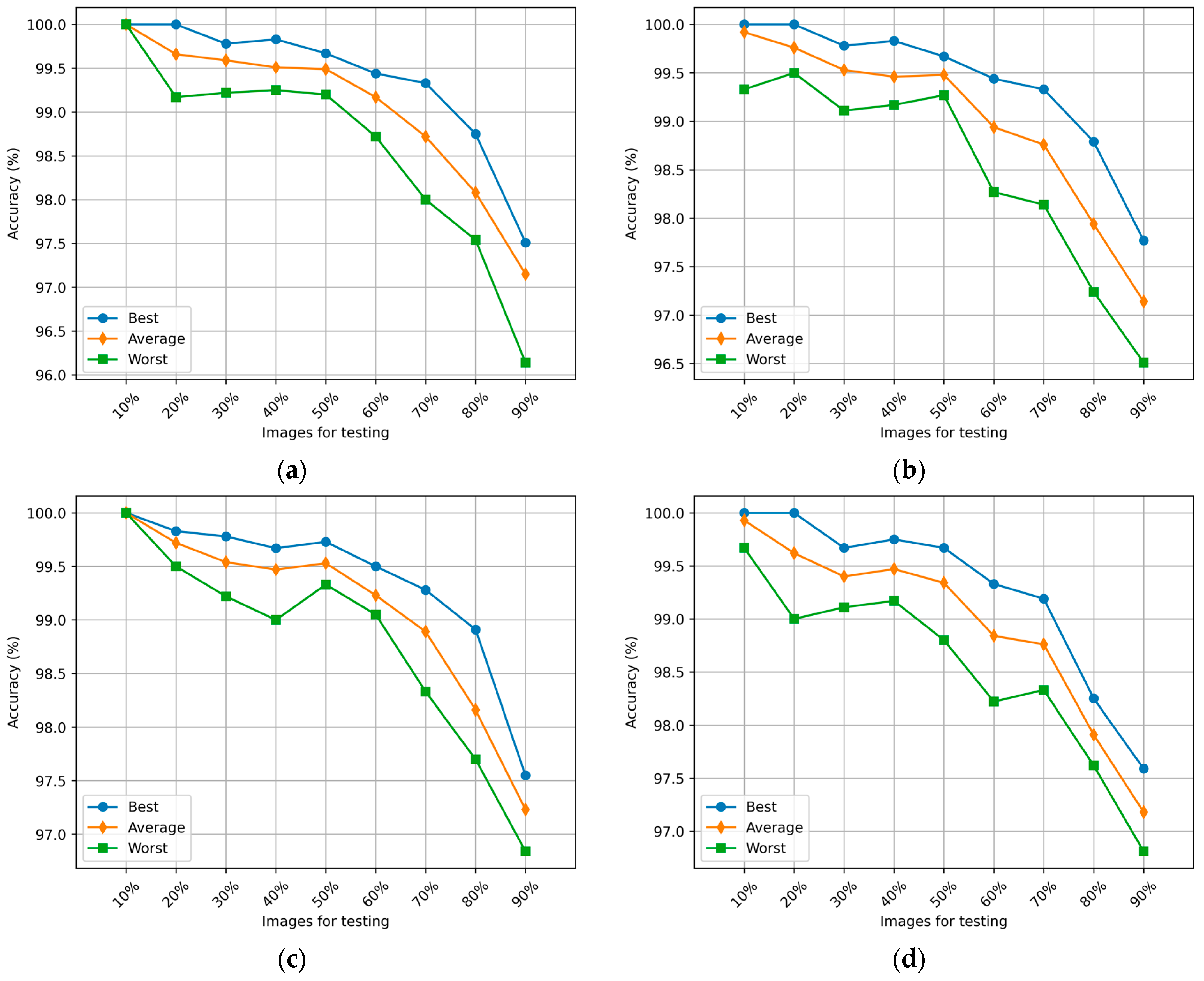
| Images (Testing) % | Best % | Average % | Worst % |
|---|---|---|---|
| 10 | - | 100 | - |
| 20 | 100 | 99.66 | 99.17 |
| 30 | 99.78 | 99.59 | 99.22 |
| 40 | 99.83 | 99.51 | 99.25 |
| 50 | 99.67 | 99.49 | 99.20 |
| 60 | 99.44 | 99.17 | 98.72 |
| 70 | 99.33 | 98.72 | 98.00 |
| 80 | 98.75 | 98.08 | 97.54 |
| 90 | 97.51 | 97.15 | 96.14 |
| % Images for Testing | CLs (Filters) | FCLs (Neurons) | Epoch | Batch Size | Error | Accuracy (%) |
|---|---|---|---|---|---|---|
| 10 | 3 | 4 | 19 | 8 | 0 | 100 |
| (9, 15, 21) | (77, 84, 83, 27) | |||||
| 20 | 5 | 5 | 20 | 32 | 0 | 100 |
| (16, 16, 32, 32, 64) | (150, 88, 150, 100, 50) | |||||
| 30 | 4 | 2 | 20 | 8 | 0.0022 | 99.78 |
| (13, 16, 32, 27) | (150, 143) | |||||
| 40 | 5 | 4 | 20 | 8 | 0.0017 | 99.83 |
| (16, 13, 32, 32, 46) | (150, 26, 136, 56) | |||||
| 50 | 5 | 5 | 20 | 8 | 0.0033 | 99.67 |
| (16, 13, 32, 32, 64) | (150, 80, 150, 100, 50) | |||||
| 60 | 5 | 5 | 20 | 16 | 0.0056 | 99.44 |
| (16, 12, 32, 32, 64) | (150, 137, 53, 55, 50) | |||||
| 70 | 4 | 4 | 20 | 8 | 0.0067 | 99.33 |
| (16, 14, 30, 32) | (150, 150, 114, 26) | |||||
| 80 | 5 | 3 | 20 | 8 | 0.0121 | 98.79 |
| (16, 9, 32, 32, 54) | (53, 150, 150) | |||||
| 90 | 3 | 3 | 20 | 8 | 0.0223 | 97.77 |
| (14, 10, 23) | (11, 96, 102) |
| Images (Testing) % | Best % | Average % | Worst % |
|---|---|---|---|
| 10 | 100 | 99.92 | 99.33 |
| 20 | 100 | 99.76 | 99.50 |
| 30 | 99.78 | 99.53 | 99.11 |
| 40 | 99.83 | 99.46 | 99.17 |
| 50 | 99.67 | 99.48 | 99.27 |
| 60 | 99.44 | 98.94 | 98.27 |
| 70 | 99.33 | 98.76 | 98.14 |
| 80 | 98.79 | 97.94 | 97.24 |
| 90 | 97.77 | 97.14 | 96.51 |
| % Images for Testing | CLs (Filters) | FCLs (Neurons) | Epoch | Batch Size | Error | Accuracy (%) |
|---|---|---|---|---|---|---|
| 10 | 3 | 3 | 14 | 16 | 0 | 100 |
| (11, 10, 28) | (121, 61, 63) | |||||
| 20 | 3 | 3 | 15 | 8 | 0.0017 | 99.83 |
| (14, 15, 20) | (66, 69, 34) | |||||
| 30 | 4 | 4 | 20 | 8 | 0.0022 | 99.78 |
| (14, 13, 17, 31) | (12, 43, 10, 75) | |||||
| 40 | 4 | 3 | 20 | 8 | 0.0033 | 99.67 |
| (15, 8, 16, 16) | (150, 150, 10) | |||||
| 50 | 4 | 5 | 20 | 8 | 0.0027 | 99.73 |
| (16, 15, 32, 24) | (150, 150, 150, 33, 28) | |||||
| 60 | 4 | 5 | 20 | 8 | 0.0050 | 99.50 |
| (15, 16, 26, 32) | (35, 150, 50, 36, 10) | |||||
| 70 | 5 | 5 | 20 | 8 | 0.0072 | 99.28 |
| (8, 8, 32, 32, 64) | (42, 150, 150, 100, 50) | |||||
| 80 | 3 | 4 | 20 | 8 | 0.0109 | 98.91 |
| (16, 8, 32) | (50, 29, 150, 100) | |||||
| 90 | 2 | 4 | 12 | 8 | 0.0245 | 97.55 |
| (12, 11) | (71, 75, 96, 25) |
| Images (Testing) % | Best % | Average % | Worst % |
|---|---|---|---|
| 10 | - | 100 | - |
| 20 | 99.83 | 99.72 | 99.50 |
| 30 | 99.78 | 99.54 | 99.22 |
| 40 | 99.67 | 99.47 | 99.00 |
| 50 | 99.73 | 99.53 | 99.33 |
| 60 | 99.50 | 99.23 | 99.05 |
| 70 | 99.28 | 98.89 | 98.33 |
| 80 | 98.91 | 98.16 | 97.70 |
| 90 | 97.55 | 97.23 | 96.84 |
| % Images for Testing | CLs (Filters) | FCLs (Neurons) | Epoch | Batch Size | Error | Accuracy (%) |
|---|---|---|---|---|---|---|
| 10 | 4 | 2 | 17 | 32 | 0 | 100 |
| (13, 8, 27, 24) | (122, 104) | |||||
| 20 | 4 | 3 | 20 | 8 | 0 | 100 |
| (10, 8, 23, 25) | (42, 139, 32) | |||||
| 30 | 3 | 2 | 10 | 8 | 0.0033 | 99.67 |
| (9, 8, 22) | (38, 93) | |||||
| 40 | 4 | 4 | 20 | 8 | 0.0025 | 99.75 |
| (16, 16, 16, 30) | (150, 67, 106, 10) | |||||
| 50 | 5 | 3 | 20 | 8 | 0.0033 | 99.67 |
| (8, 9, 32, 19, 64) | (120, 81, 10) | |||||
| 60 | 4 | 5 | 20 | 8 | 0.0067 | 99.33 |
| (9, 12, 16, 29) | (63, 10, 53, 15, 15) | |||||
| 70 | 4 | 3 | 16 | 8 | 0.0081 | 99.19 |
| (8, 8, 26, 32) | (14, 102, 37) | |||||
| 80 | 3 | 1 | 15 | 8 | 0.0175 | 98.25 |
| (16, 13) | (48) | |||||
| 90 | 1 | 4 | 11 | 8 | 0.0241 | 97.59 |
| (15) | (107, 131, 117, 53) |
| Images (Testing) % | Best % | Average % | Worst % |
|---|---|---|---|
| 10 | 100 | 99.93 | 99.67 |
| 20 | 100 | 99.62 | 99.00 |
| 30 | 99.67 | 99.40 | 99.11 |
| 40 | 99.75 | 99.47 | 99.17 |
| 50 | 99.67 | 99.34 | 98.80 |
| 60 | 99.33 | 98.84 | 98.22 |
| 70 | 99.19 | 98.76 | 98.33 |
| 80 | 98.25 | 97.91 | 97.62 |
| 90 | 97.59 | 97.18 | 96.81 |
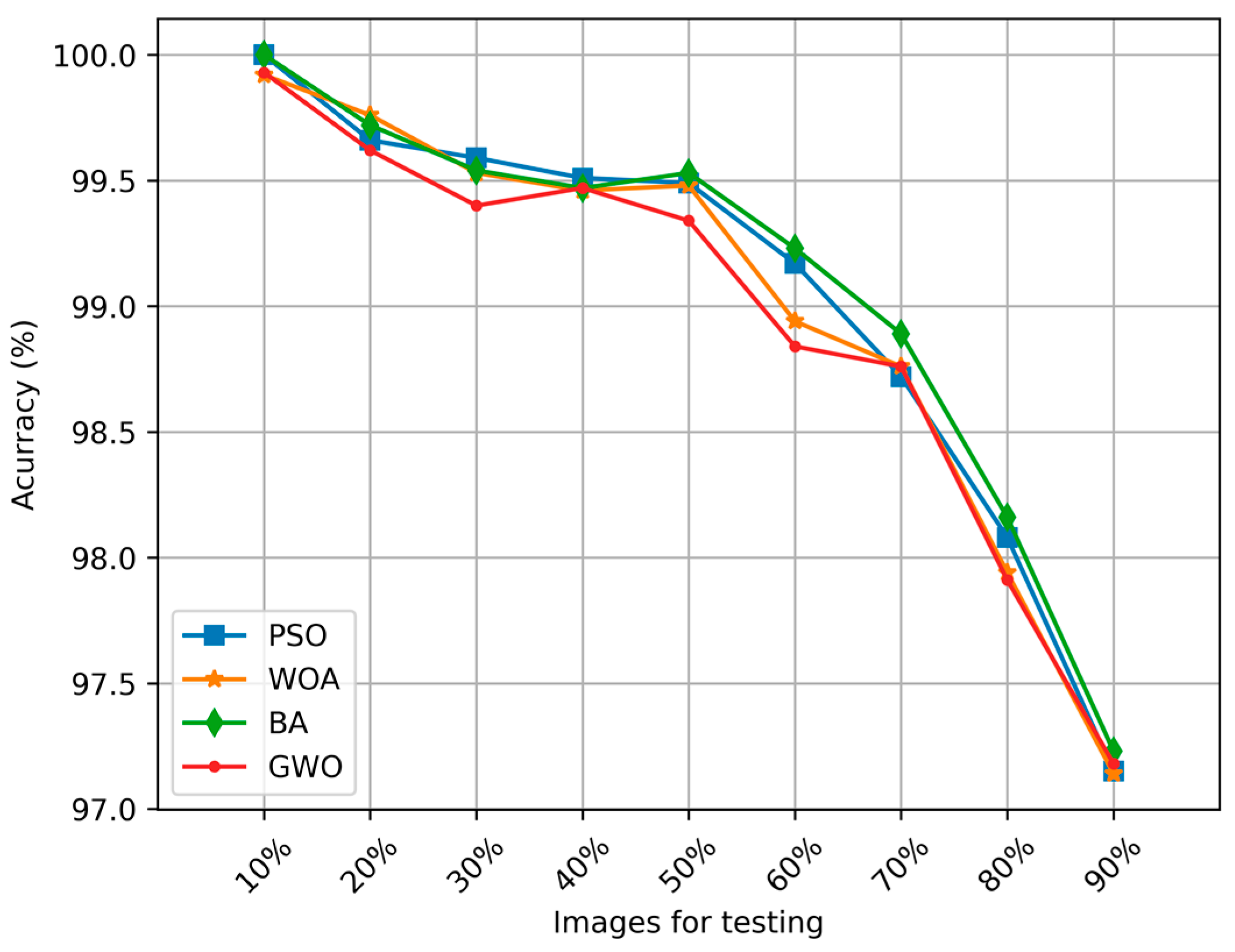
| Images (Testing) % | PSO % | WOA % | BA % | GWO % |
|---|---|---|---|---|
| 10 | 100 | 99.92 | 100 | 99.93 |
| 20 | 99.66 | 99.76 | 99.72 | 99.62 |
| 30 | 99.59 | 99.53 | 99.54 | 99.40 |
| 40 | 99.51 | 99.46 | 99.47 | 99.47 |
| 50 | 99.49 | 99.48 | 99.53 | 99.34 |
| 60 | 99.17 | 98.94 | 99.23 | 98.84 |
| 70 | 98.72 | 98.76 | 98.89 | 98.76 |
| 80 | 98.08 | 97.94 | 98.16 | 97.91 |
| 90 | 97.15 | 97.14 | 97.23 | 97.18 |
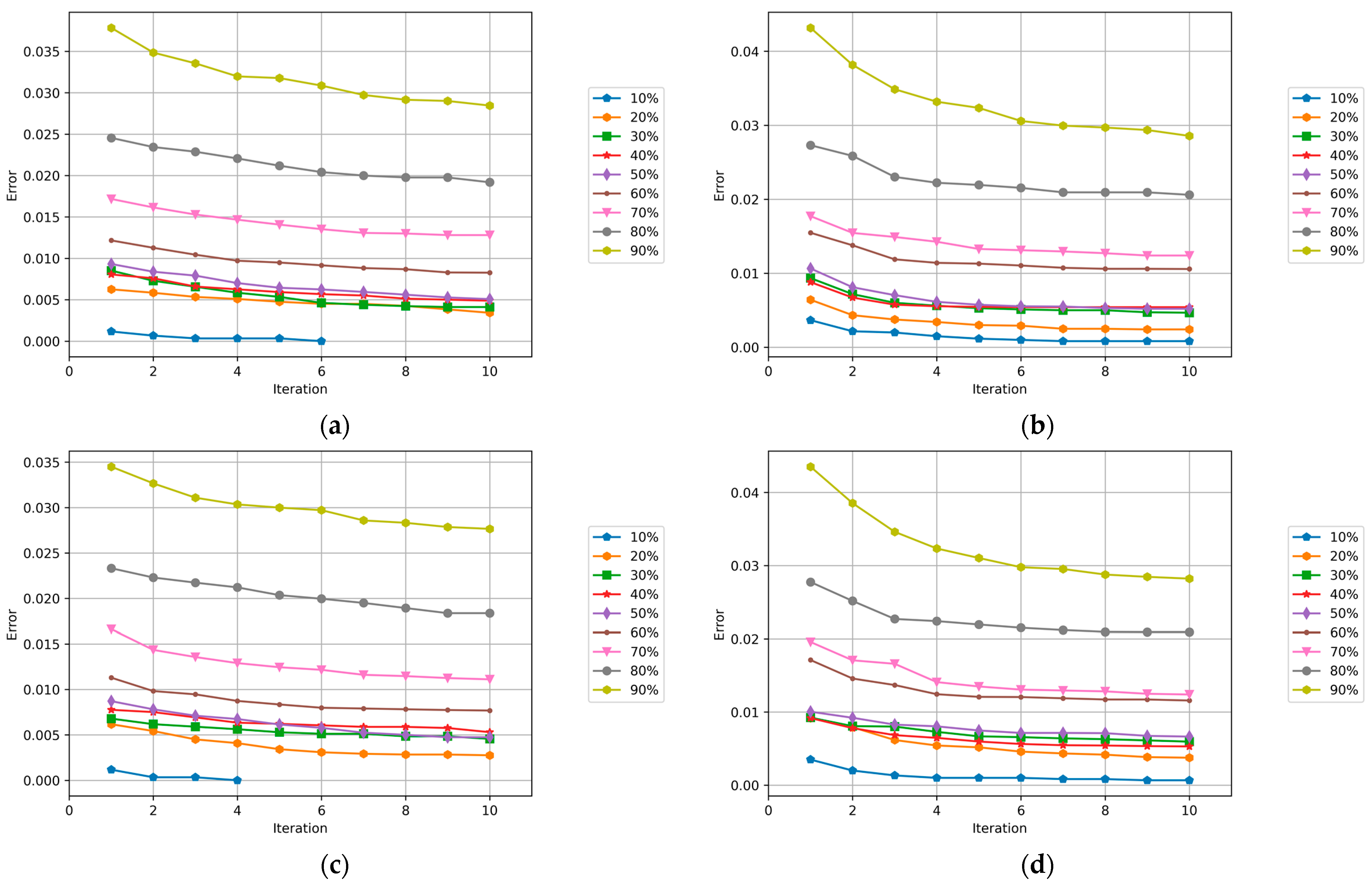
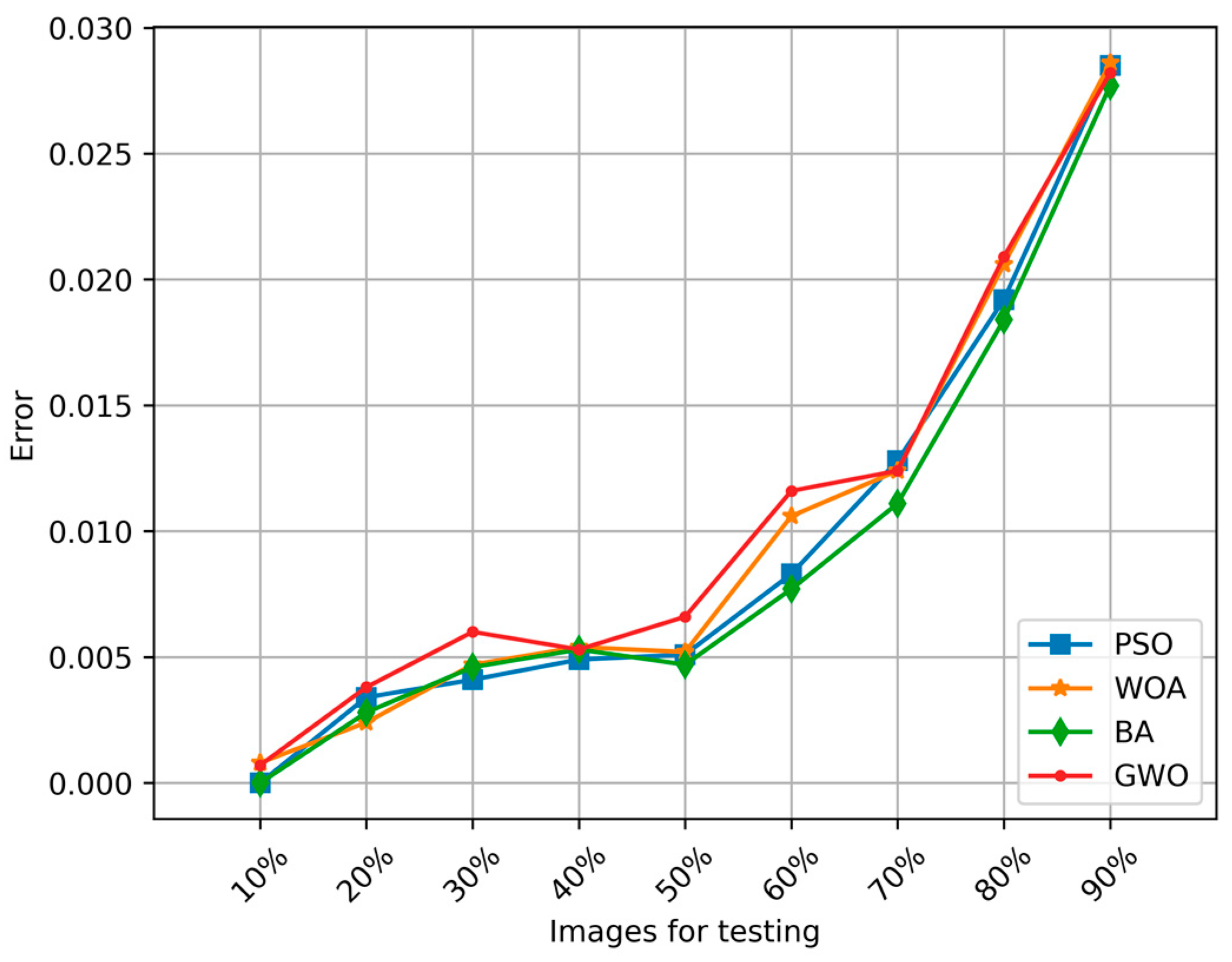
| % Images (Testing) | PSO | WOA | BA | GWO |
|---|---|---|---|---|
| 10 | 0 | 0.0008 | 0 | 0.0007 |
| 20 | 0.0034 | 0.0024 | 0.0028 | 0.0038 |
| 30 | 0.0041 | 0.0047 | 0.0046 | 0.006 |
| 40 | 0.0049 | 0.0054 | 0.0053 | 0.0053 |
| 50 | 0.0051 | 0.0052 | 0.0047 | 0.0066 |
| 60 | 0.0083 | 0.0106 | 0.0077 | 0.0116 |
| 70 | 0.0128 | 0.0124 | 0.0111 | 0.0124 |
| 80 | 0.0192 | 0.0206 | 0.0184 | 0.0209 |
| 90 | 0.0285 | 0.0286 | 0.0277 | 0.0282 |
| Metric | PSO | WOA | BA | GWO |
|---|---|---|---|---|
| Accuracy | 100 | 99.92 | 100 | 99.93 |
| Recall | 97.05 | 96.28 | 99.77 | 95.80 |
| Precision | 80.07 | 82.67 | 84.47 | 81.38 |
| F1 Score | 86.18 | 87.31 | 90.54 | 86.40 |
| n | α | ||
|---|---|---|---|
| 0.02 | 0.05 | 0.10 | |
| 9 | 3 | 6 | 8 |
| Methods | Negative Sum (W−) | Positive Sum (W+) | Test Statistic (W) | Degrees of Freedom (m) | W0 = Wα,m |
|---|---|---|---|---|---|
| BA PSO | 41 | 3 | 3 | 9 | 8 |
| BA WOA | 41 | 3 | 3 | 9 | 8 |
| BA GWO | 44 | 0 | 0 | 9 | 8 |
| PSO WOA | 34 | 10 | 10 | 9 | 8 |
| PSO GWO | 39 | 5 | 5 | 9 | 8 |
| WOA GWO | 33 | 10 | 10 | 9 | 8 |
Disclaimer/Publisher’s Note: The statements, opinions and data contained in all publications are solely those of the individual author(s) and contributor(s) and not of MDPI and/or the editor(s). MDPI and/or the editor(s) disclaim responsibility for any injury to people or property resulting from any ideas, methods, instructions or products referred to in the content. |
© 2023 by the authors. Licensee MDPI, Basel, Switzerland. This article is an open access article distributed under the terms and conditions of the Creative Commons Attribution (CC BY) license (https://creativecommons.org/licenses/by/4.0/).
Share and Cite
Melin, P.; Sánchez, D.; Pulido, M.; Castillo, O. Comparative Study of Metaheuristic Optimization of Convolutional Neural Networks Applied to Face Mask Classification. Math. Comput. Appl. 2023, 28, 107. https://doi.org/10.3390/mca28060107
Melin P, Sánchez D, Pulido M, Castillo O. Comparative Study of Metaheuristic Optimization of Convolutional Neural Networks Applied to Face Mask Classification. Mathematical and Computational Applications. 2023; 28(6):107. https://doi.org/10.3390/mca28060107
Chicago/Turabian StyleMelin, Patricia, Daniela Sánchez, Martha Pulido, and Oscar Castillo. 2023. "Comparative Study of Metaheuristic Optimization of Convolutional Neural Networks Applied to Face Mask Classification" Mathematical and Computational Applications 28, no. 6: 107. https://doi.org/10.3390/mca28060107