1. Introduction
In a practical multi-objective optimization study, users should have the flexibility in choosing a dominance structure which would involve objective preferences and priorities of users. In most evolutionary multi-objective optimization (EMO) studies, a set of Pareto-optimal solutions are attempted to be found by an evolutionary population-based algorithm and the choice of a single preferred solution from the Pareto-optimal set is deferred as a post-optimality decision-making task [
1,
2]. In the recent past, some exceptions to this principle have shown that a generic dominance structure can be created with desired preference information for the resulting EMO to converge to a single preferred Pareto-optimal solution or to focus to a preferred Pareto-optimal region at the end of the optimization task [
3,
4,
5,
6,
7]. The practicalities and merits of both approaches from computational and decision-making points of view can be debated, but if the preference information is easier to obtain, the latter approach can be appealing from a computational viewpoint.
The EMO and classical optimization literature has proposed a number of alternate dominance structures for this purpose [
8,
9,
10,
11,
12], not always motivated by the decision-making preferences used in the real world, rather from considering interesting geometric constructions aided by their practical significance. However, the literature lacks a systematic study outlining what properties a generalized dominance structure must have such that an EMO will end up finding a non-empty optimal solution set with certain desired properties. This study attempts to fill this gap and answer the following questions. Does any arbitrarily chosen dominance structure generate a non-empty optimal solution set? For a given dominance structure, how does one identify the resulting optimal solution set for a problem? If a dominance structure fails to produce an optimal solution, are there ways to modify it to find the desired non-empty optimal solution set? To have confidence in the derived principles, do they reveal known properties of the existing dominance structures?
To achieve our goal, we have formalized the concept of an anti-dominance structure, which is intricately dependent on the chosen dominance structure; however, we argue that it is more useful than the dominance structure in answering the above questions and providing a better understanding of the outcome of the chosen dominance structure. In addition to the conditions for a non-empty optimal solution set, we discover a number of interesting and useful properties of these structures to determine if the respective optimal solution set has a single optimum or multiple optima. Contrary to the general belief, it has been clearly demonstrated here that dominance structures satisfying semi-transitive properties can lead to an optimal solution set and that a satisfaction of the transitive property need not be a hard restriction. Although demonstrated using two- and three-objective problems in this paper, the concepts of this paper are applicable to many-objective problems as well. Overall, the results of this paper should enable researchers to obtain a better insight into a direct understanding of generalized dominance structures and the resulting optimal solution set, which may be useful in achieving various EMO activities, such as multi-objective test problem generation, efficient algorithm development with a knowledge of sources of algorithmic inefficiencies in finding the true optimal solution set, and the design of meaningful generalized dominance structures for effective application.
In the rest of the paper, we discuss the optimality conditions for single-objective optimization problems in a generalized manner through an inferior structure concept in
Section 2. Based on uni-modal and multi-modal single-objective optimization, the concept of an anti-inferior structure is introduced so the concept of inferior and anti-inferior (or anti-dominance) structures can be carried over to multi-objective optimization in
Section 3.
Section 4 applies the concept of an anti-dominance structure to explain the working of a number of existing generalized dominance principles proposed in the literature. Then, in
Section 5, we extend the use of dominance and anti-dominance structures for spatially changing dominance relationships. Finally, in
Section 6, we present the conclusions of this study.
2. Optimality Principles for Single-Objective Optimization
For a single-objective minimization problem:
in which
is the variable vector,
is the objective function, and
is the
j-th inequality constraint. A solution is called
feasible if all
J constraints are satisfied by the solution. Let us denote the feasible solution set
as the set of all feasible solutions in the search space and the feasible objective set
. If a solution is not feasible, it is called an
infeasible solution.
To arrive at the definition of the optimal solution for the problem stated above, we first define the concept of the inferiority solution set of a feasible solution . Every member of is worse than in terms of the given objective function. To understand the inferiority set, we first define the inferiority condition between two feasible solutions.
Definition 1 (Single-objective inferiority condition). For a pair of feasible solutions and , is inferior to (or mathematically, ) in a single-objective sense if .
From this condition, we derive an inferior solution set , as follows:
Definition 2 (Single-objective inferior set of ). The set of all feasible solutions for which is defined as the inferior set of , and the set of respective objective values is defined as the inferior objective set .
For minimization problems, the inferior objective set of
can also be written as follows:
The summation is in the Minkowski sense. For a problem, the user can provide a generalized
null inferior structure
at the origin to define the desired inferiority condition (
). Note that the definition of
may not depend on the knowledge of the feasible objective space
and can be defined purely based on the desired condition for a generalized “optimal” solution. The following relationships between
and
can be written:
The above inferiority condition respects the following properties:
Irreflexive property: A solution is not inferior to itself, that is, .
Asymmetric property: If , then .
Transitive property: If and , then .
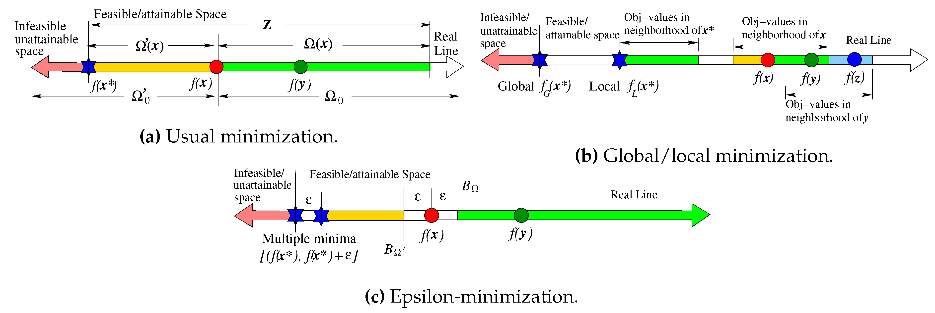
Graphically, the above inferiority condition can be demonstrated with a sketch of the objective function on a real line (
), as shown in
Figure 1a. In the sketch,
represents the entire green line on the right of
, excluding the value of
.
Note that a simple check on is not adequate for defining an optimal solution appropriately, particularly if there exist multiple optimal solutions to the problem. To define the optimal solution, we need to define an anti-inferior solution set and its corresponding anti-inferior objective set as follows:
Definition 3 (Anti-inferiority condition). For a pair of feasible solutions and , is anti-inferior to in a single-objective sense if .
A little thought will lead us to define the
anti-inferior solution set
and the
anti-inferior objective set . For the sketch in
Figure 1a, the golden line left of
(excluding
) denotes the anti-inferior objective set. The set
is important in determining the optimal solution, as there cannot exist any better solution than the optimal solution:
Definition 4 (Single-objective optimality condition). A solution is an (global) optimal solution in the single-objective sense if its anti-inferior objective set is empty or .
For the solution
in
Figure 1a,
(there is no feasible objective value left of
). Hence, it is an optimal solution to the problem. This is true for every global optimal solution. The opposite is also true.
Theorem 1 (Empty anti-inferior set). If is an (global) optimal solution, its anti-inferior set is empty, or, .
The proof is intuitive. The definition and theorem also suggest that at the optimal solution , . From the asymmetric property, it is also true that for every feasible point . However, this may not be true at every feasible point in the search space and still have an existence of an optimal solution by satisfying . However, if this condition is not met at every feasible point, an algorithm to find optimal solutions may have difficulties in progressing towards the optimal region.
Let us now define a null anti-inferior structure at the origin as , so that and . It is interesting to note from their mathematical constructs that . Because the user has the liberty to choose any null inferior structure for defining certain desired properties of the resulting optimal solution(s), it is advisable to meet the condition to guarantee asymmetric property everywhere in the search space, irrespective of the nature of . This may allow the smooth operation of an optimization algorithm. However, in some esoteric cases, an optimal solution still may exist without satisfying this condition with . This happens when there exists no feasible solution at the overlapping region of inferior and anti-inferior structures applied at the optimal solution. This discussion brings us to the following theorem.
Theorem 2 (Overlapping inferior and anti-inferior sets). For a null inferior structure with non-empty , an optimal solution exists only if .
Note that the Definition 4 is also valid for each of the multiple global optimal solutions if they exist in a problem, as all such optimal solutions have an identical value. However, for a local optimal solution, the condition needs to be appended with a local neighborhood restriction of , , around .
Definition 5 (Single-objective local inferiority condition). For a pair of feasible solutions and , is local inferior to (say, ) in a single-objective sense if .
Figure 1b marks the respective objective values in the neighborhood of
. It is understood that
is within a radius of
around
and has a worse objective value than
, hence
in the local sense. Note that the anti-inferior solution and objective sets for a local optimal solution can also be defined by restricting the members within the neighborhood. For brevity, we do not define them here. The irreflexive and asymmetric properties are still valid for the local inferior structure; however, the transitivity property may not be satisfied among three feasible solutions (
,
, and
). To have
, the solution
must be in the neighborhood of
, and to have
, the solution
must be in the neighborhood of
; however, these conditions do not require that
must be in the neighborhood of
. Hence,
may not lie in
, and vice versa. Thus, the transitivity property may not be satisfied for the local inferiority structure. This brings us to the semi-transitive property for a generic inferiority structure:
It is not as strong as the transitive property. This property does not require that the solution be better than , but enforces that must not be better than . Clearly, if an inferiority structure does not satisfy the transitivity property, it must necessarily satisfy the semi-transitive property for it to break the inferiority cycle and finally result in an optimal solution.
Theorem 3 (Nonexistence of optimum). If both transitive and semi-transitive properties are violated by an inferiority structure, there cannot exist an optimal solution.
Proof. This can be proven by contradiction. Assume that there exists an optimal solution and also consider two other feasible solutions and , in which satisfies and satisfies . Because neither the transitivity nor semi-transitivity condition is satisfied, it is possible that and , thereby violating the optimality condition stated in Definition 4. □
2.1. Epsilon-Inferiority Conditions
Let us reconsider Equation (
2) and generalize it with a non-negative parameter
(Equation (
2) was defined with
):
Equation (
5) allows a generalization of the inferior objective set with an epsilon-optimality condition in which a solution
is considered epsilon-inferior to
, if
, allowing a more practice-oriented inferiority definition, as shown in
Figure 1c. Writing
in terms of the difference in objective values (
), we can define a
null inferior set,
. Thus,
in the Minkowski sense. The defining boundary of the inferior set
(
in this case) is an important feature for a user to define the desired inferiority of a solution in the feasible objective set
. The boundary of the inferior set can be inclusive (
) to the set or exclusive (
). Note that the epsilon-inferiority condition defined in Equation (
5) is valid for
.
It is interesting to note that the respective anti-inferior objective set is
, where
is the null anti-inferior set for the epsilon-inferior condition. In the same manner as before, we notice that
. All solutions
which have an objective value smaller than
from
are now epsilon-inferior to
. The defining boundary of the anti-inferior set is
for the epsilon-inferiority definition.
Figure 1c shows that solutions with objective values left of
are inferior to
. By definition, irreflexive, asymmetric, and transitive properties are satisfied by the epsilon-inferiority structure.
The epsilon-inferiority condition extends the definition of optimality conditions for problems having multiple optimal solutions. All solutions which are within from the optimal solution’s objective value are epsilon-optimal. This discussion helps to define optimality conditions for multi-objective optimization.
3. Optimality Principles for Multi-Objective Optimization
A constrained multi-objective optimization problem having
M conflicting objectives,
J inequality constraints, and no equality constraints is formulated as follows:
The set of feasible solutions satisfying all constraints is denoted with and the respective objective vectors constitute the feasible objective set . First, we extend and define the inferiority of a solution over another as follows:
Definition 6 (Multi-objective inferiority condition). For a pair of solutions and , is inferior to in a multi-objective sense if dominates ().
The above requires a suitable definition of dominance. The popularly used Pareto-dominance condition () is defined as follows:
Definition 7 (Pareto-dominance() condition). A solution Pareto-dominates another solution , if the following two conditions are true: (i) for all , and (ii) for at least one .
Note that for the single-objective case, and the above dominance condition becomes equivalent to the inferiority condition defined in Definition 1. As with the single-objective case, the inferior objective set is defined as follows: . To define the optimality condition (Pareto-optimality condition with ), we need to have the definition of anti-inferior objective set , derived from a generalized dominance structure .
It is clear from the above discussion that the dominance concept between two solutions prevalent in multi-objective optimization literature is equivalent to the inferiority concept introduced here for single-objective optimization. Hence, we call
and
sets the
dominance and
anti-dominance sets of
, respectively, in the context of multi-objective optimization. Like in the single-objective case, a user can define the null dominance structure
, a bounded
M-dimensional set for which origin is not a member for multi-objective optimization. The resulting dominance set at a point
is then defined as
. Clearly,
.
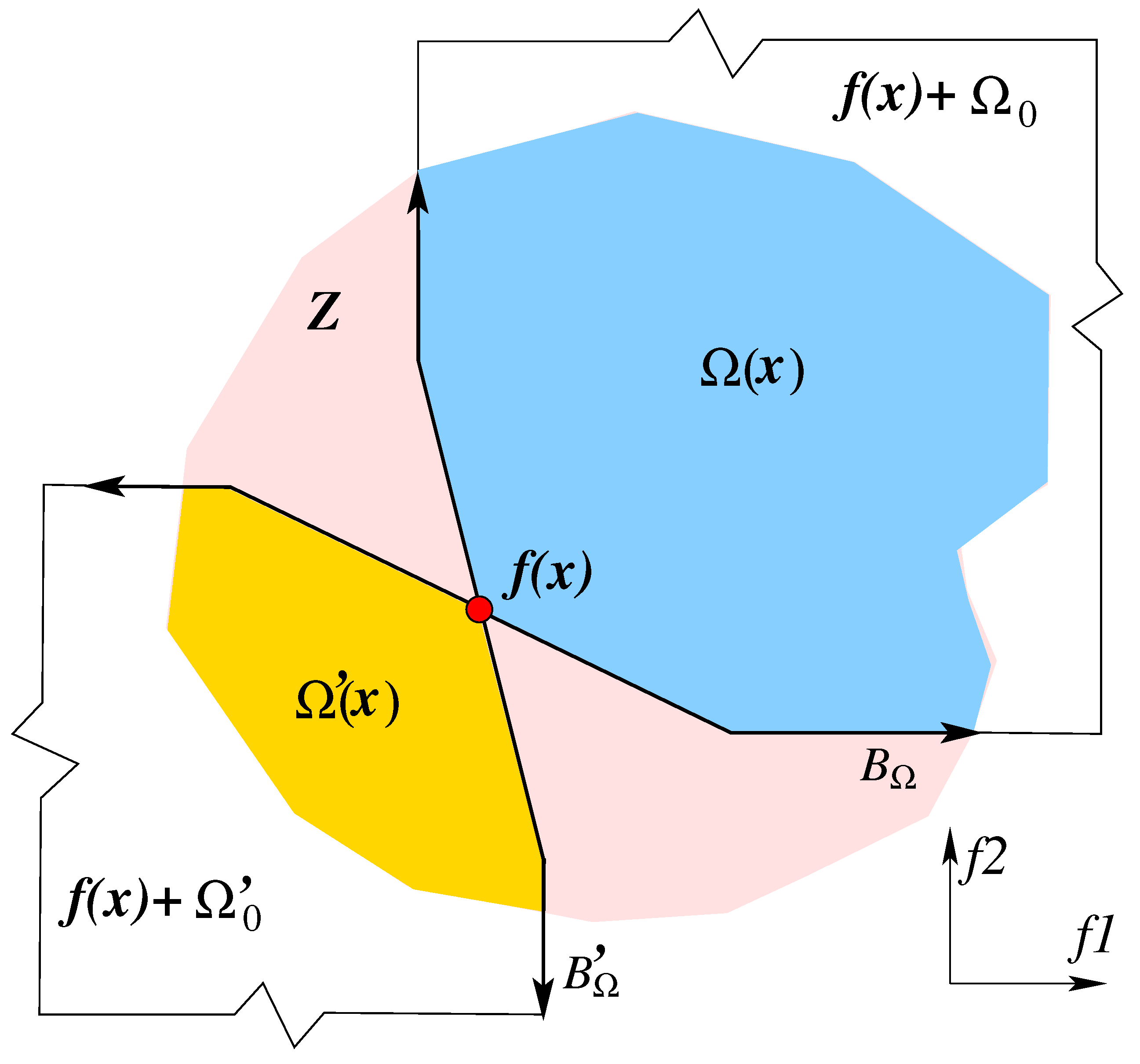
Figure 2 shows a specific dominance structure and its null structure. The boundary
of
in the
M-dimensional objective space can be obtained from
. Then, the resulting null anti-dominance structure
can be determined from
with a procedure described in
Section 3.2 in order to define the respective generalized optimal solutions for the supplied dominance structure
. Extending the concept from single-objective optimization, the defined generalized dominance structure must satisfy irreflexive and asymmetry properties mentioned for the single-objective case and also the transitivity or semi-transitivity property stated in Theorem 3.
Knowing the null anti-dominance structure and defining anti-dominance objective set , an optimal solution for a multi-objective optimization problem can be defined as follows:
Definition 8 (Multi-objective optimality condition). A solution is optimal in the multi-objective sense with a generalized dominance structure at the origin if there does not exist any feasible solution in the anti-inferior objective set, or .
The resulting objective vector lies in the optimal set . Note that the above definition can result in multiple optimal solutions. In fact, if the optimal solution of the single-objective constrained optimization problem with the i-th objective function is different from () that of j-th objective function, then and can both occur. Both solutions then become optimal solutions to the multi-objective optimization problem. Besides these individual optimal solutions, many other compromise solutions, trading off the objectives, may exist in the feasible solution set. For the Pareto-dominance structure () with , the respective optimal solutions are called Pareto-optimal solutions () and the set is referred to as the Pareto-optimal set. The respective set of objective vectors (set ) is called to constitute a Pareto-optimal front (PF), in the parlance of the EMO literature.
As with Theorem 1 for the single-objective case, the following is also true:
Theorem 4 (Empty anti-dominance set for multi-objective optimization). If is an optimal solution, its anti-inferior objective set is empty, or, .
Although it is advisable to construct a dominance structure such that to achieve a smooth progress of an optimization algorithm towards the optimal region, for some scenarios, an overlapping and structure can also cause an optimal solution to exist, particularly when , meaning that there does not exist any other feasible objective vector other than the optimal objective vector at the intersection of dominance and anti-dominance objectives sets constructed at the optimal solution.
3.1. Defining a Generalized Dominance Structure for Multi-Objective Optimization
The defining boundary for the dominance structure is useful to define a generalized dominance condition for the multi-objective case. Extending the boundary of the dominance structure
discussed for epsilon-inferiority condition in
Section 2.1, one can define a boundary
at the origin to declare the part of the
M-dimensional objective space (with
-vector) that are dominated (or worse) than the origin, where
is the vector of changes in objective values.
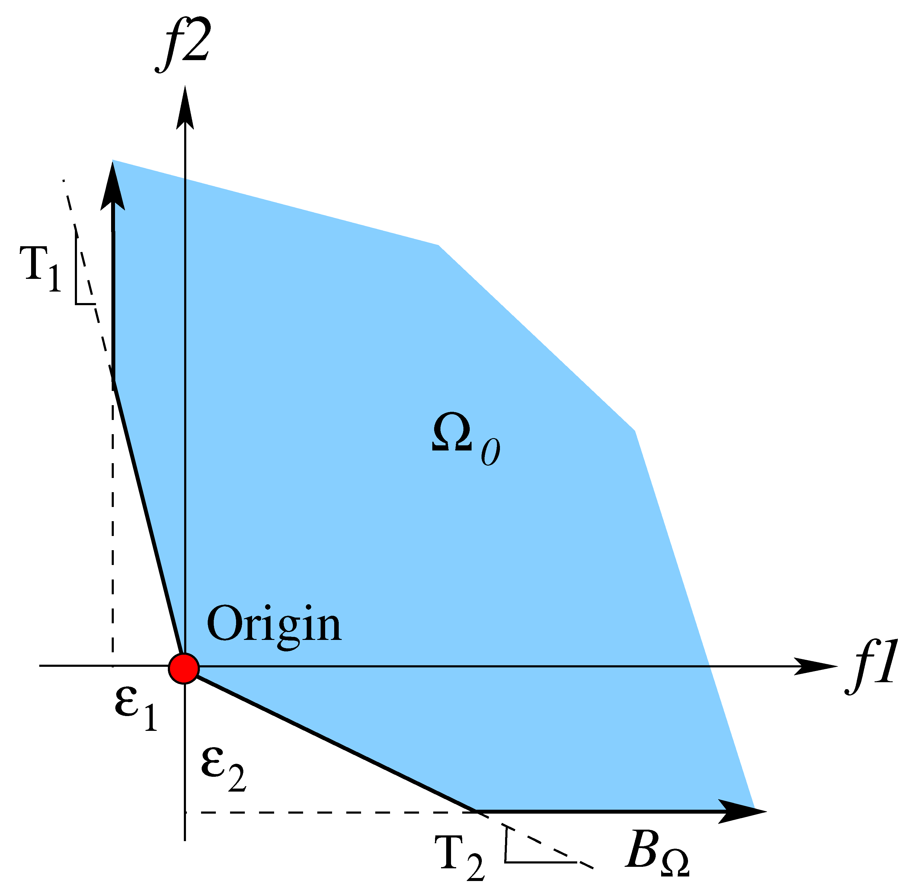
Figure 3 shows one such generalized dominance structure (
) at the origin. It implies that, up to a limit of
change on
from the origin, the origin is inferior to any point with a trade-off (loss/gain) larger than
. A similar trade-off of
exists for a limit of
change in
. Note that the generic
structure allows any arbitrary definition of the dominance structure as a function of changes in objectives, compared to the objective-wise settings in the level sets [
13] and epsilon-dominance principles [
14]. A redefinition of the dominance structure will create a different set of optimal solutions than the Pareto-optimal solutions. Hence, such an approach will allow users to find respective optimal solution set for any chosen dominance structure. However, before we find the generalized optimal solution set, let us find the relationship between
and
.
3.2. Relationship between Dominance and Anti-Dominance Structures
Every member of the dominance structure is dominated by (i.e., worse than) the origin and every member of anti-dominance structure dominates (i.e., is better than) the origin. As indicated for the single-objective case, the two sets are related by a simple relation: . The following theorem states that this is a universal property, even for the multi-objective case.
Theorem 5 (Relationship between dominance and anti-dominance structures). For any null dominance set , its null anti-dominance structures .
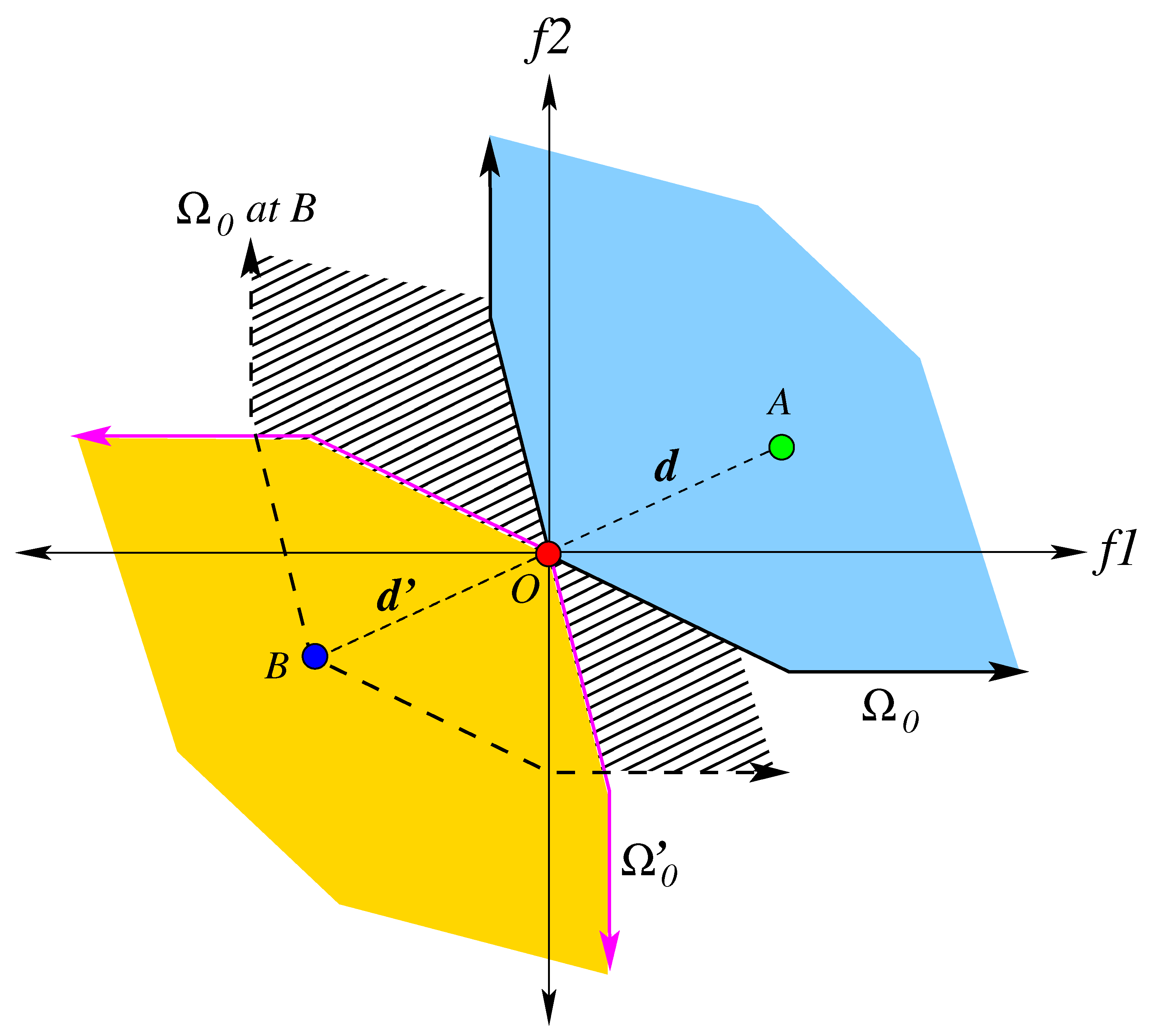
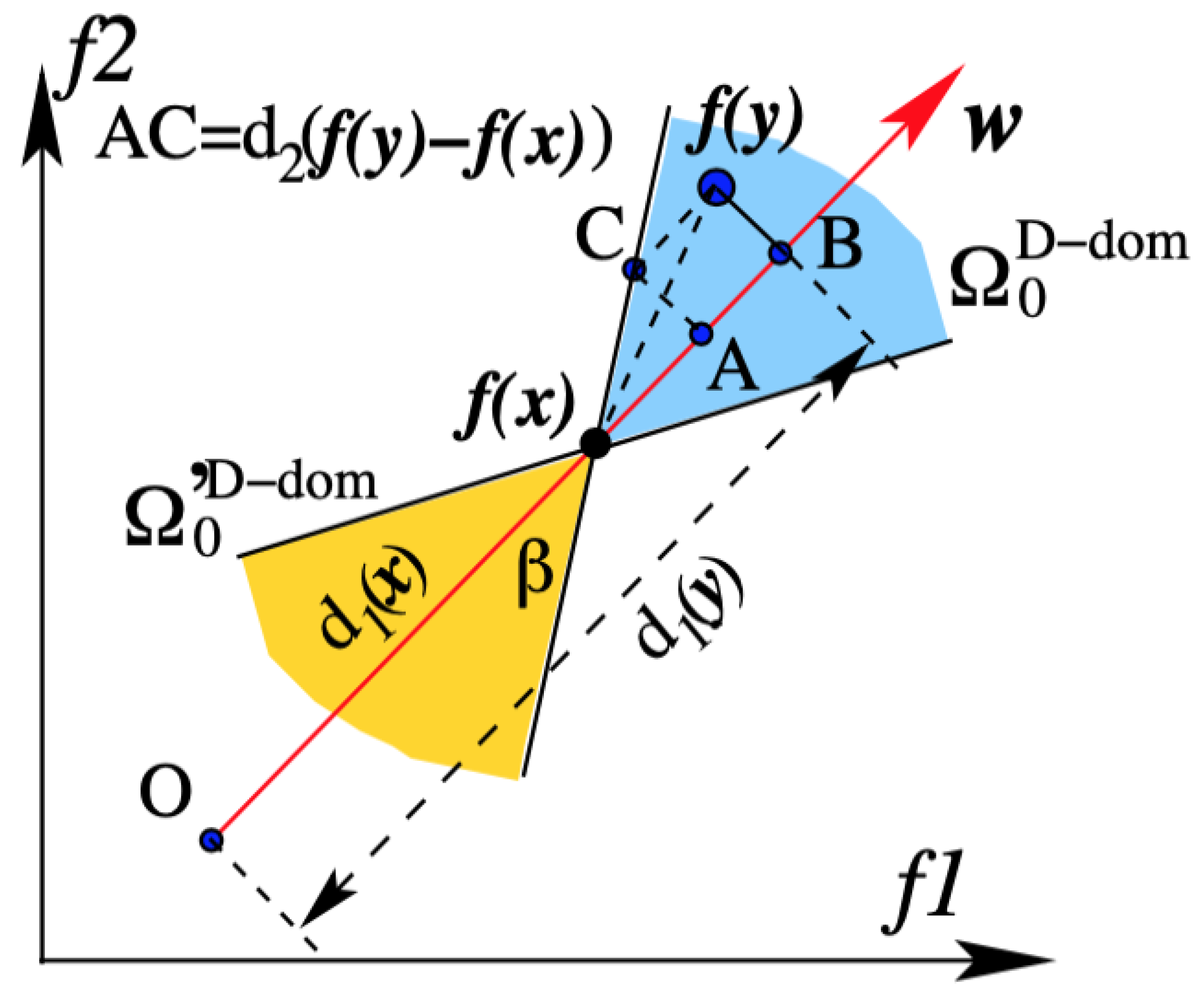
Proof. Let us consider
Figure 4 for a proof with a generic dominance structure (
) defined at the origin (point O). Let us consider a generic point A at
from O. Let us now construct a point B at
from O. Now, we construct the dominance structure
at B (shown in shaded region), as if B is the new origin. Then, the original origin (point O) is now at
location from the new origin (B). Because
is inside the set
, the new origin B dominates the original origin O. This is true for every
, and thus
can be constructed with negative vectors of every member of
. □
Corollary 1. For any dominance structure with a defining boundary , the defining boundary of the anti-dominance structure .
As with the single-objective case, we now discuss the properties that a generalized dominance (GD) structure () must have:
Irreflexive property: (and its boundary ) must exclude the -vector (origin) from its set.
Asymmetric property: (recommended, as discussed in the paragraph before Theorem 2).
Transitive property: This requires a chain of
consideration and requires further discussion (provided in
Section 3.2.1).
The first two properties indicate that a GD structure can have an inclusive boundary with points on the boundary being inferior to the origin or an exclusive boundary on which the points are not inferior to the origin.
The above also indicates the following corollary is true, as in multi-objective objective space, overlapping solutions between and can arise from the boundary () of the chosen dominance structure:
Corollary 2. For , if , no optimal solution exists.
The clause indicates that boundary must be included in both and . Because this contradicts , the corollary is true. For , the clause is true only when (origin). Because the definition of excludes the origin, the corollary may not be true for .
Corollary 3. If , the exclusive boundaries must be equal (that is, ) and all optimal solutions must lie on passing through one of the optimal solutions.
The above theorem is valid for the exclusive boundary GDs. The weighted-sum dominance structure (Figure 9d) satisfies the above condition and forces all optimal solutions to lie on the boundary plane
having a normal vector (
) and passing through any of the optimal solutions
. Another GD structure is shown in
Figure 5.
3.2.1. Transitive and Semi-Transitive Properties
It has been previously mentioned that the generalized dominance structure
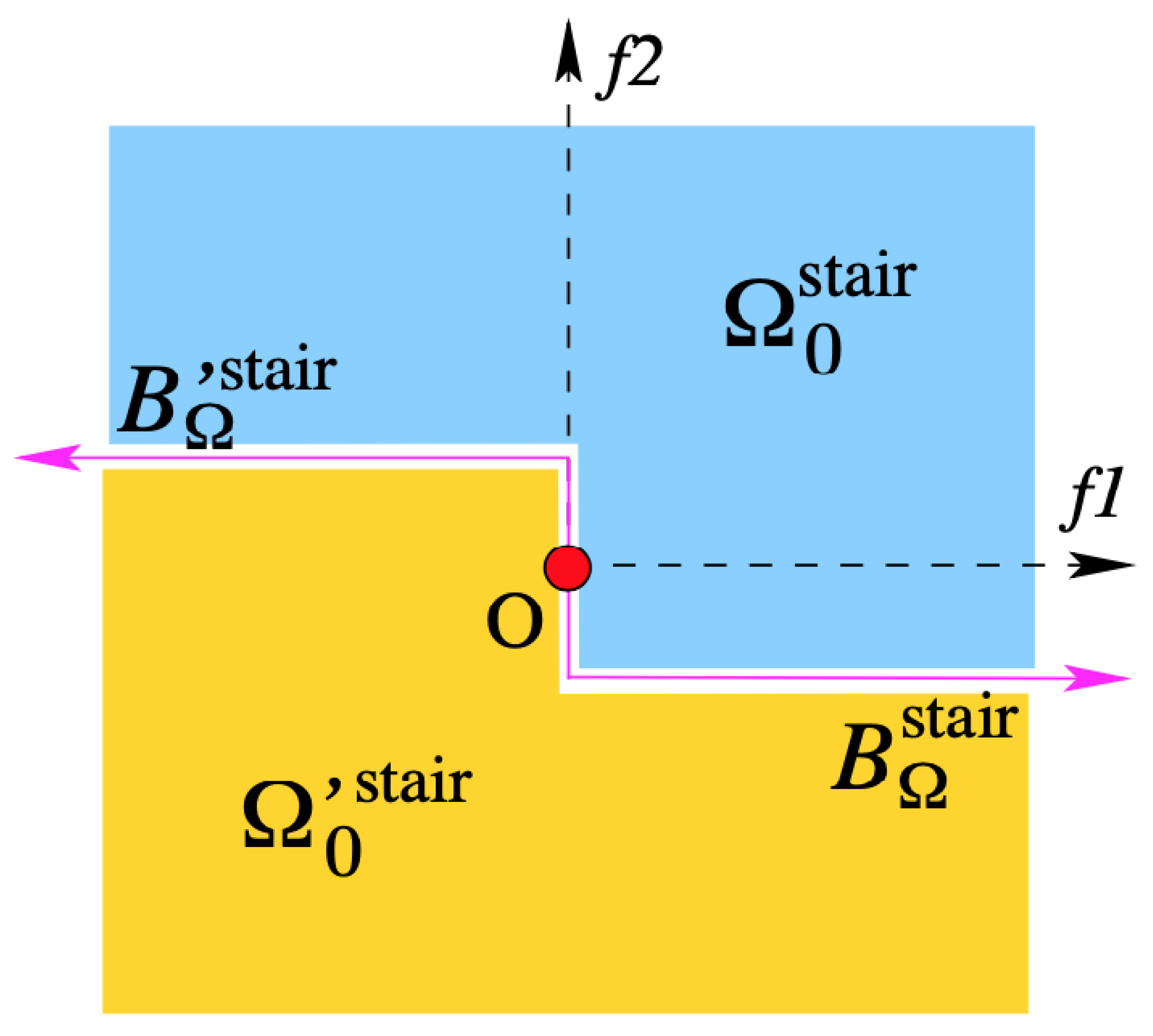
having irreflexive, asymmetric, and semi-transitive properties can produce a non-empty optimal solution set, contrary to the general belief that a transitive property is a must. Let us first demonstrate this fact graphically with the generalized dominance structure considered in
Figure 3. We observe from
Figure 6 that when a dominated or an inferior point
is chosen from
at
and another point
is chosen from
at
,
may not dominate
, in general. This violates the transitive property, but we observe from the figure that this specific dominance structure satisfies the semi-transitive property in that
does not dominate
, as
does not lie inside the
set. Thus, an important task is to determine the true nature of the
effective dominance structure when intermediate points such as
are allowed in the optimization process.
For a population-based optimization algorithm, such as evolutionary multi-objective optimization (EMO) [
1,
2], the set of non-dominated population members (which are not dominated by any other population member) is determined by comparing every population member with every other for dominance. Thus, in an EMO population, if all three solutions (
,
, and
) exist,
will not be in the same non-dominated set with
due to the presence of
as a
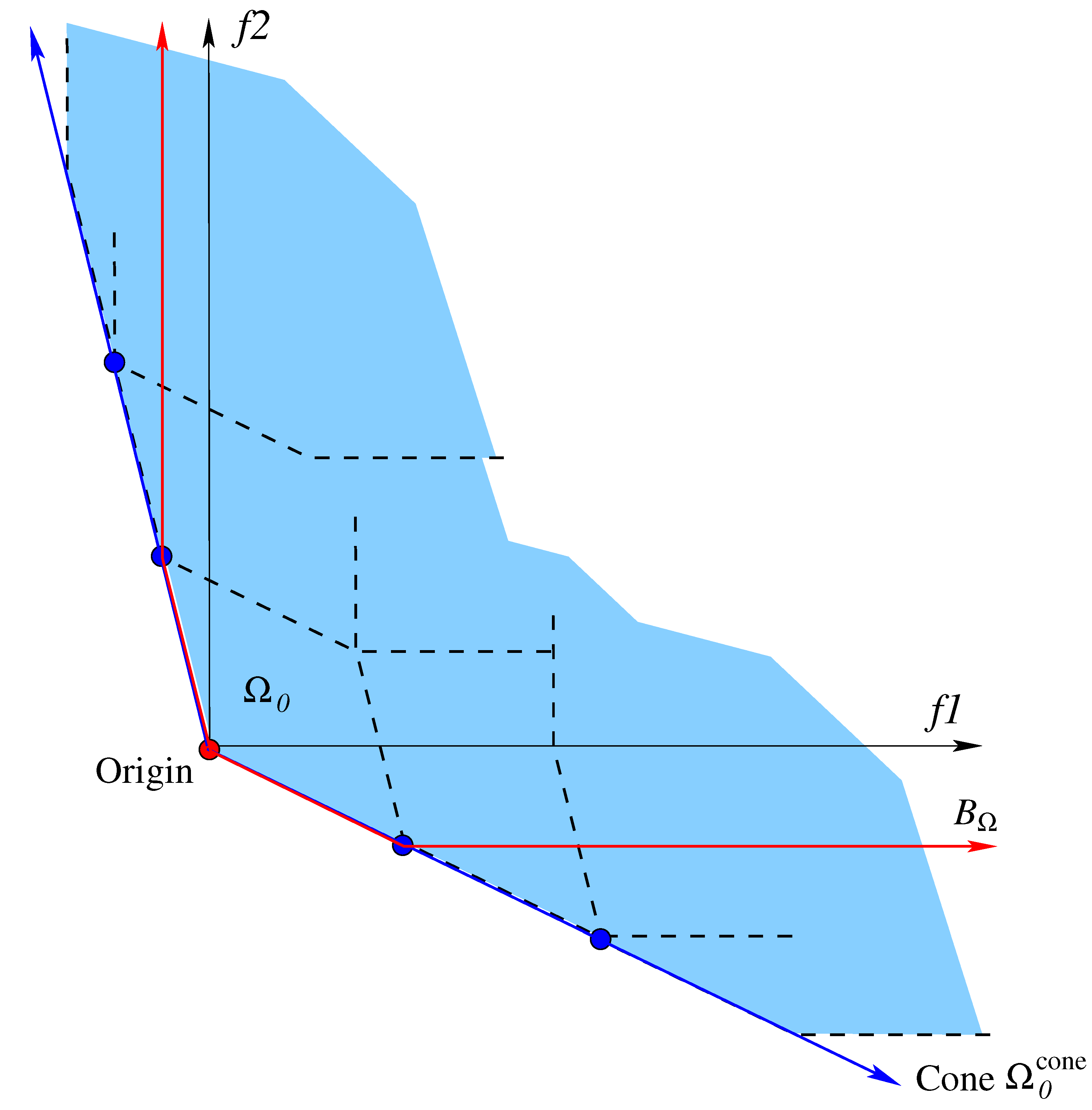
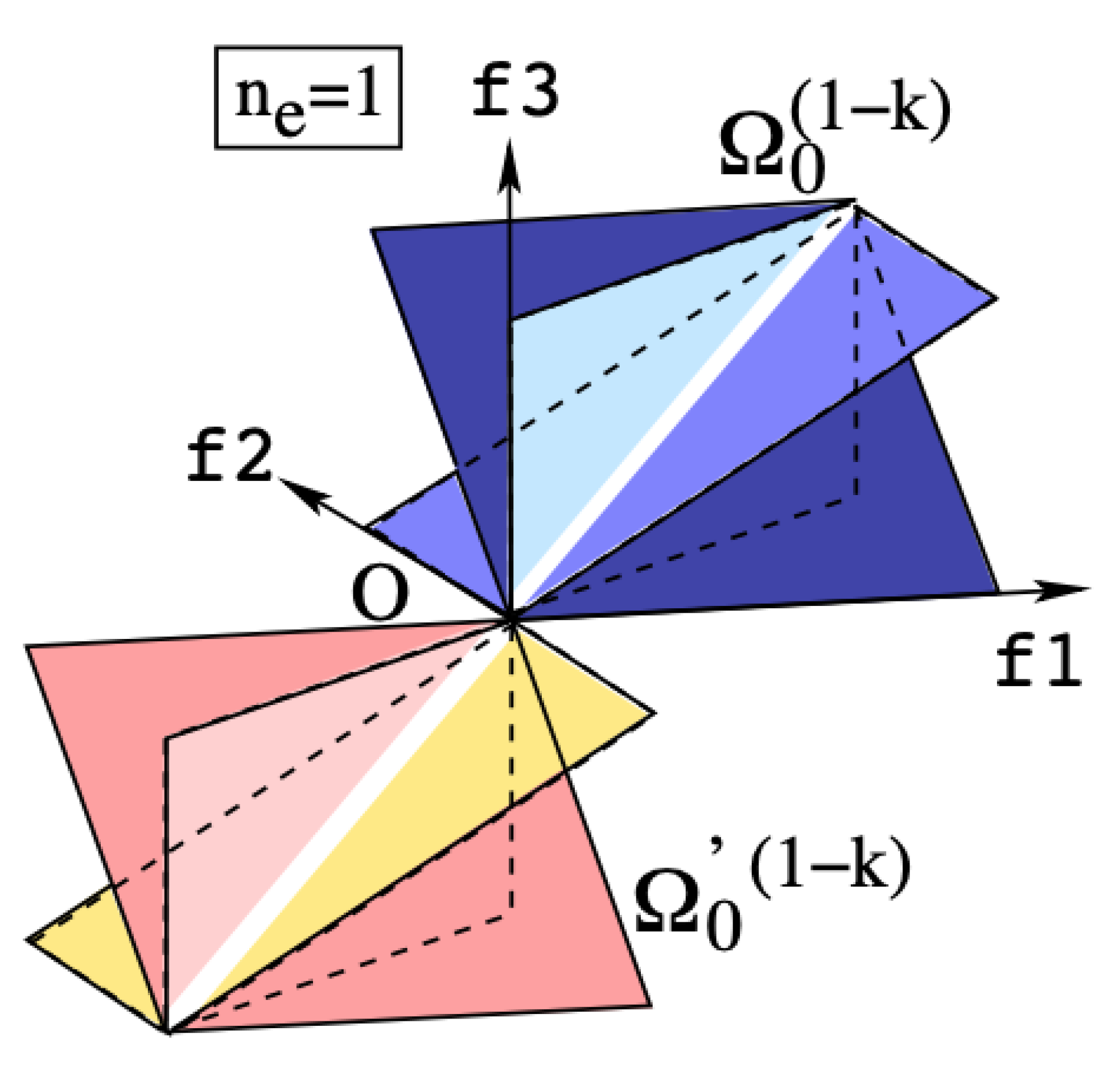
catalyst in the population. This may not be possible for a point-based multi-objective optimization approach, which works mostly by comparing two competing solutions at every iteration. If we continue the chain of dominance structure on the specific problem in
Figure 3, we observe that with the presence of catalyst solutions, the effective dominant structure of
becomes a cone, shown in
Figure 7, which has the transitive property [
13].
This example illustrates how a semi-transitive dominance (STD) structure can exhibit an effective transitive dominance (ETD) structure in the presence of a population of catalyst solutions, such as solution . This is an important distinction between population-based and point-based multi-objective optimization algorithms, allowing EMO researchers and practitioners to consider a more relaxed dominance structures to suit their practical needs. This concept leads to the following theorem.
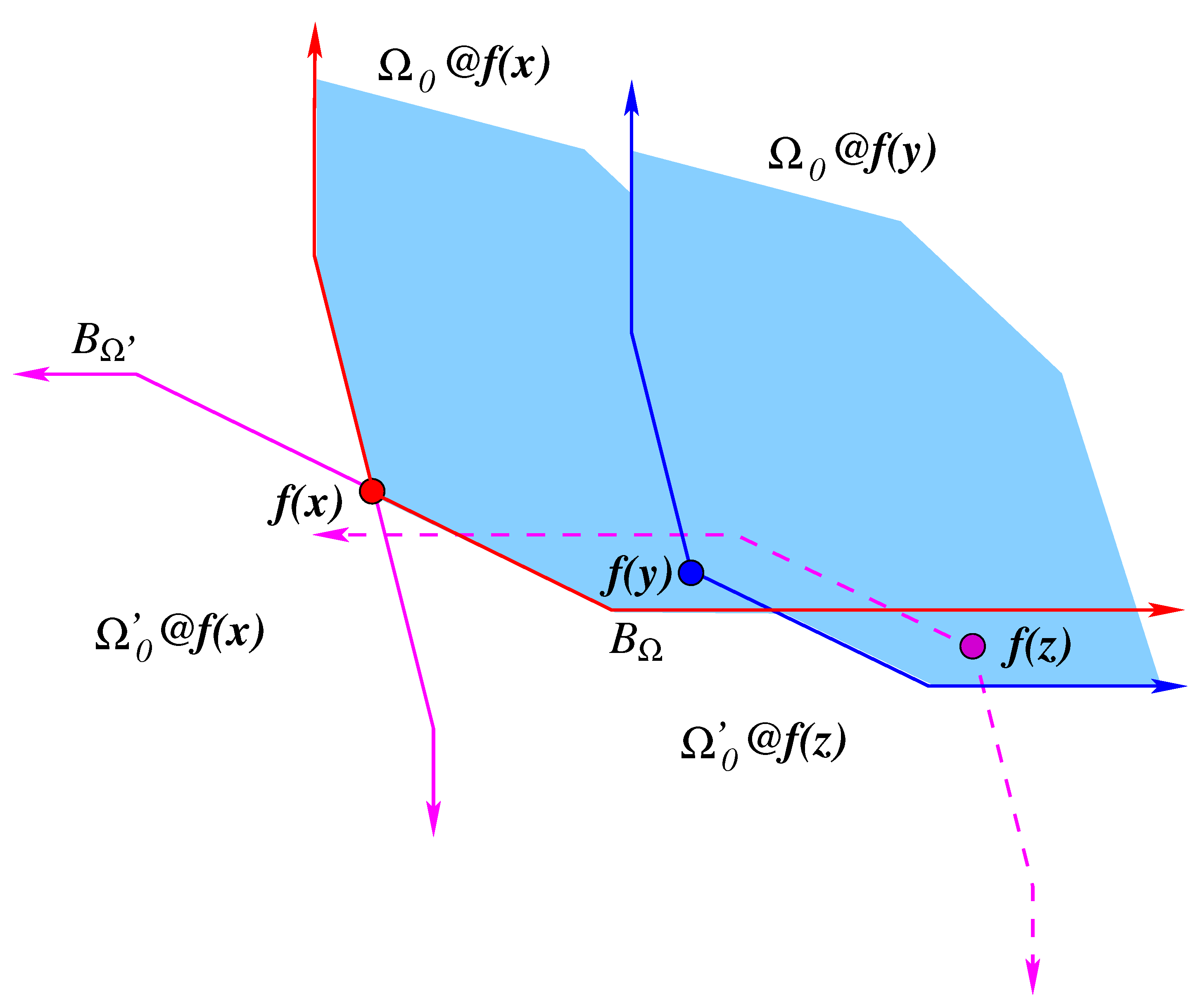
Theorem 6 (Semi-transitive and effective transitive dominance structure relation). For a semi-transitive dominance structure having , its effective transitive dominance structure also follows the same principle: .
Proof. Consider three points
,
, and
in
Figure 6. The semi-transitive property indicates that
, and
, but
. The final property indicates that
cannot lie in
of
. Clearly,
and
of
, as the ETD structure is the collection of all such dominated points, thereby yielding
. If
must lie in
as well, it means that there exists a chain of points starting with
, making
and
. Because each and every point
which is dominated by
is also a member of
(by semi-transitive property of GD structure),
. Hence, the chain breaks, and
cannot be a member of both
and
. □
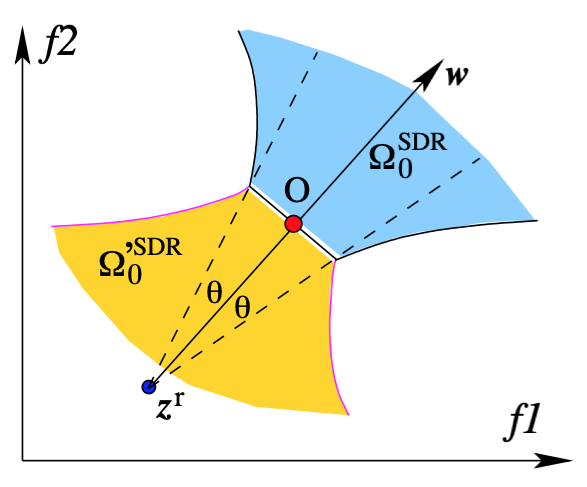
3.2.2. Further Illustration of Semi-Transitive Property
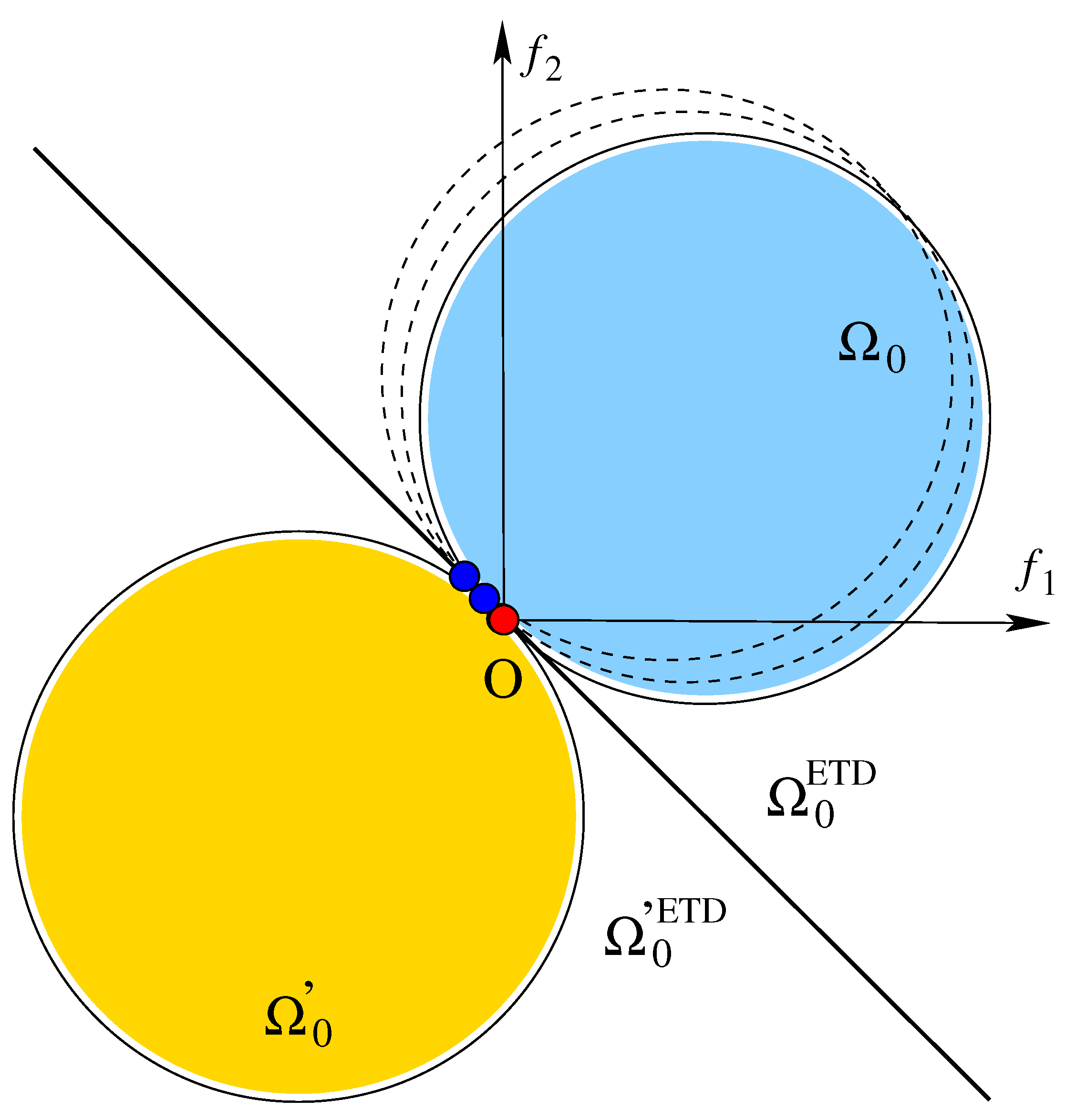
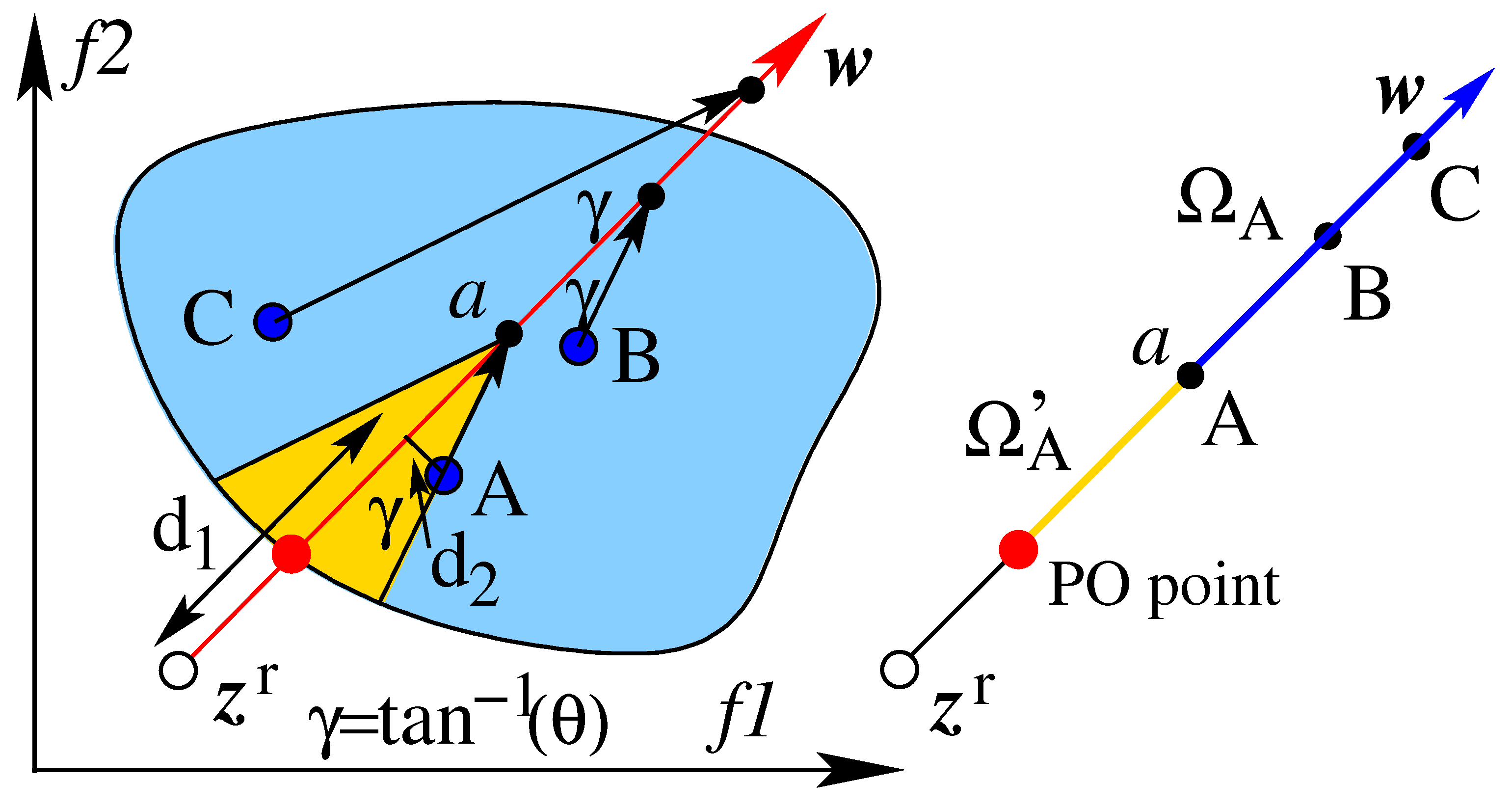
Let us define a circle-dominance structure
at the origin indicating the region inside (and not on) the blue circle, which is dominated by the origin, as shown in
Figure 8. The origin is at
radian from the positive
-axis set at the center of the circle. Its anti-dominance structure
is shown in golden color. Clearly,
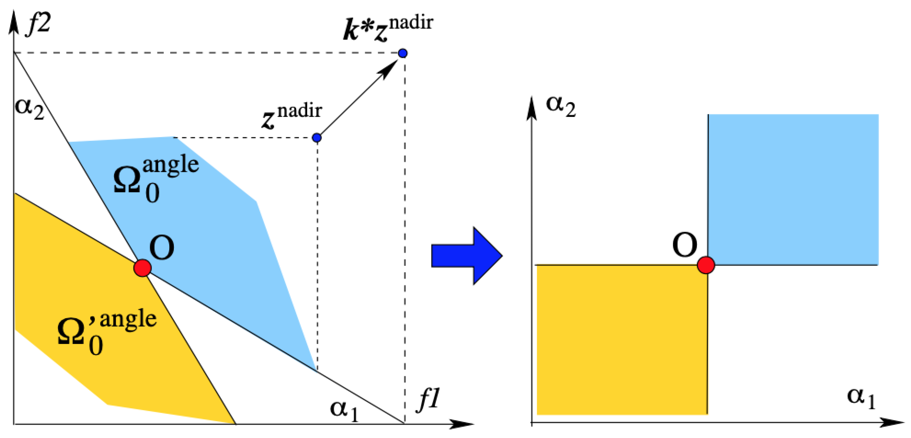
. Thus, this circle dominance structure is expected to produce a non-empty optimal solution set. However, to understand the exact nature of the optimal solution set, we notice that the above circle dominance structure is semi-transitive. An analysis reveals that the effective transitive dominance (ETD) structure is a region above the
line at the origin:
, shown in the figure. The respective anti-dominance structure is
. A careful thought reveals that the ETD structure is identical to the weighted-sum dominance structure with equal weight to each objective and according to Theorem 6, the respective ETD and anti-ETD structures are also non-overlapping. Thus, although we wanted to establish a circle-dominance concept to find respective optimal points, an EMO will effectively establish a weighted-sum dominance structure with equal weight to find the optimal points. Thus,
with equal weights.
For semi-transitive dominance structures, the results (both theoretical and experimental) of this paper extend to their effective transitive dominance structures as well.
3.3. Commonly Used Dominance Structures
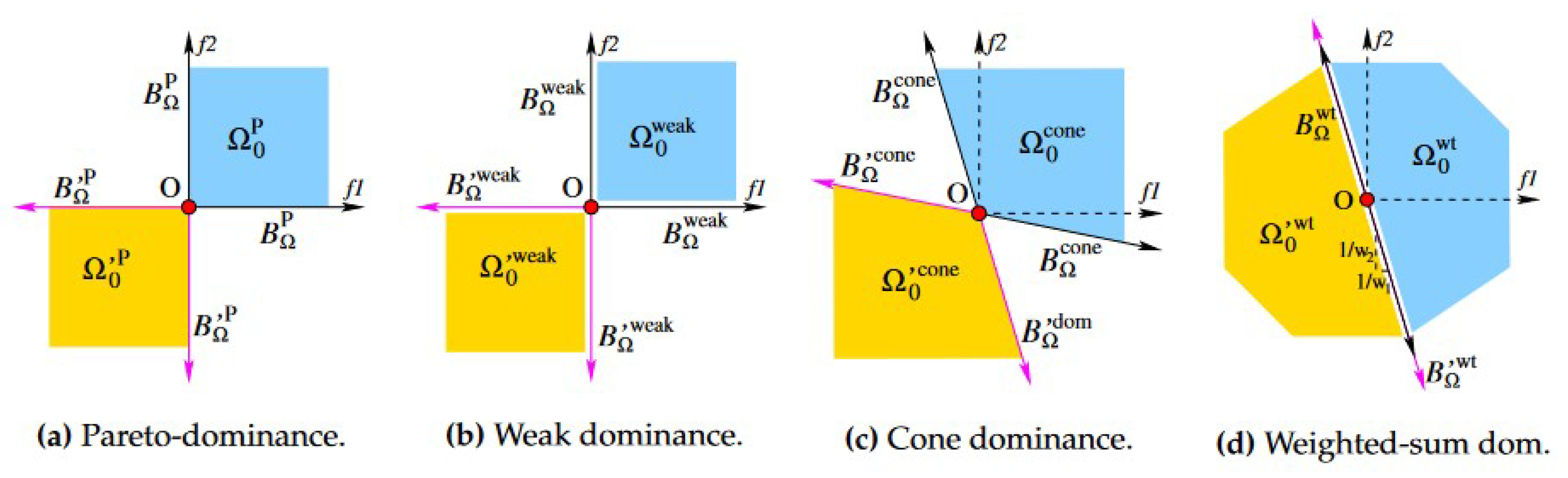
Figure 9 shows
for a number of commonly used dominance structures in the literature and presents their respective
set for two-objective problems. They are extendable to higher dimensions as well.
First, the Pareto-dominance structure (
), in which the origin dominates all points in its first quadrant (for two objectives) without itself, is shown in
Figure 9a. Its respective
is, by definition, the third quadrant without the origin. Because
(second and fourth quadrants are not in the set
, hence the subset symbol ⊂), the optimal solution set is likely to have multiple optimal points.
Second, the weak dominance structure (
), in which a point dominates all points in the interior of its first quadrant (for two objectives), is shown in
Figure 9b. Its respective
is the interior of the third quadrant.
Next,
and its respective
of the commonly used cone dominance structure [
13,
15] are shown in
Figure 9c. Note that for a wider cone structure (cone angle more than 180 degrees for two objectives), the asymmetric property is violated, meaning
. Such a structure will result in an empty optimal solution set.
For the weighted-sum approach,
, the resulting
and is shown
Figure 9d. Here,
. According to Corollary 3, the optimal point(s) must lie on the hyperplane boundary
passing through one of the optimal solutions.
We discuss a few more existing generalized dominance structures in
Section 4, but next we discuss an important matter of identifying the generalized optimal solution set for a given generalized dominance structure.
3.4. Identifying Generalized Non-Dominated Set
For a given structure, a member of the generalized non-dominated (GND) set in a finite population of objective vectors P is defined as follows:
Definition 9 (Generalized non-dominated set). A feasible objective vector in a finite set P is a member of the generalized non-dominated set with a null GD structure if no other member of P lies in the anti-dominance set at , or .
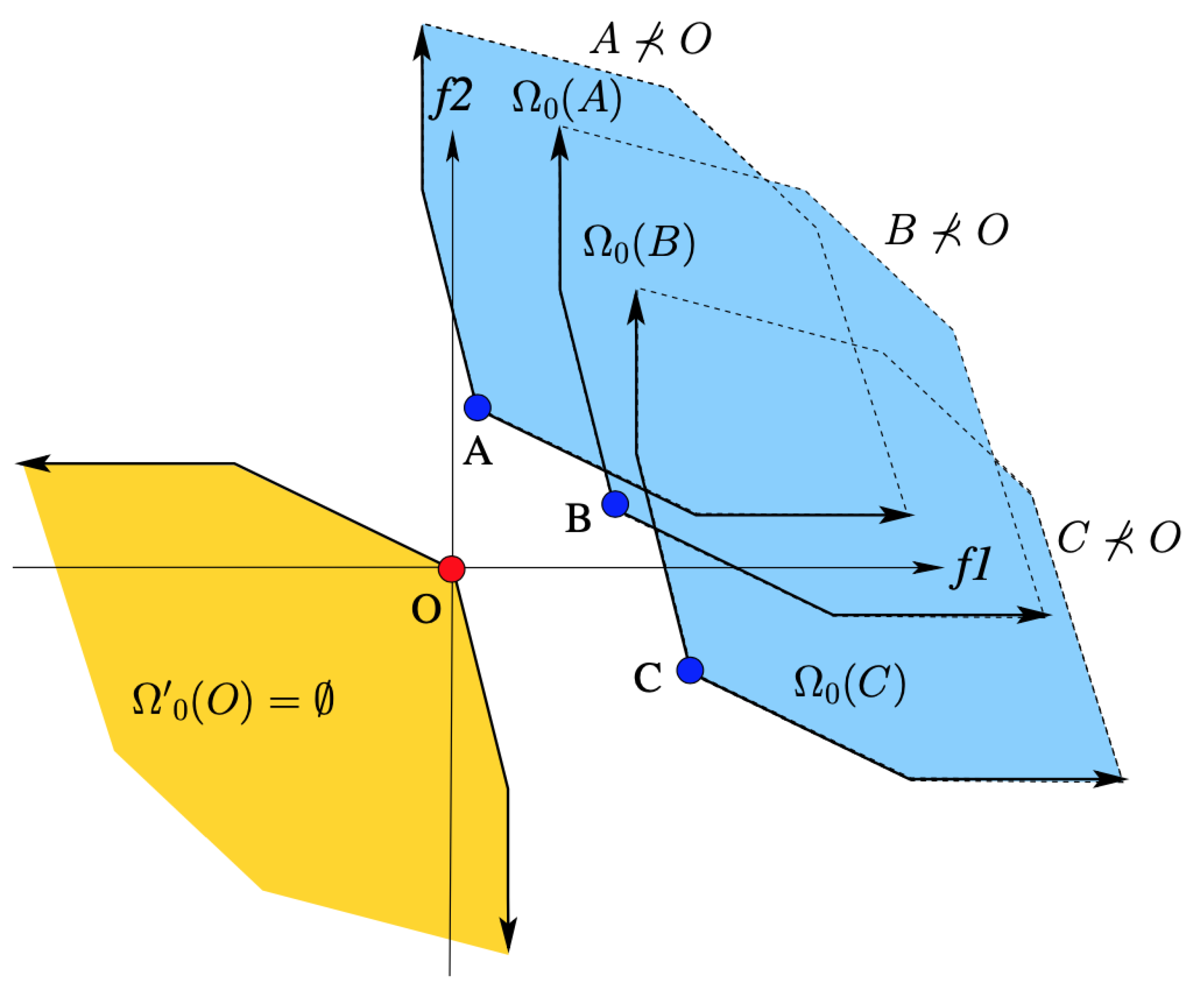
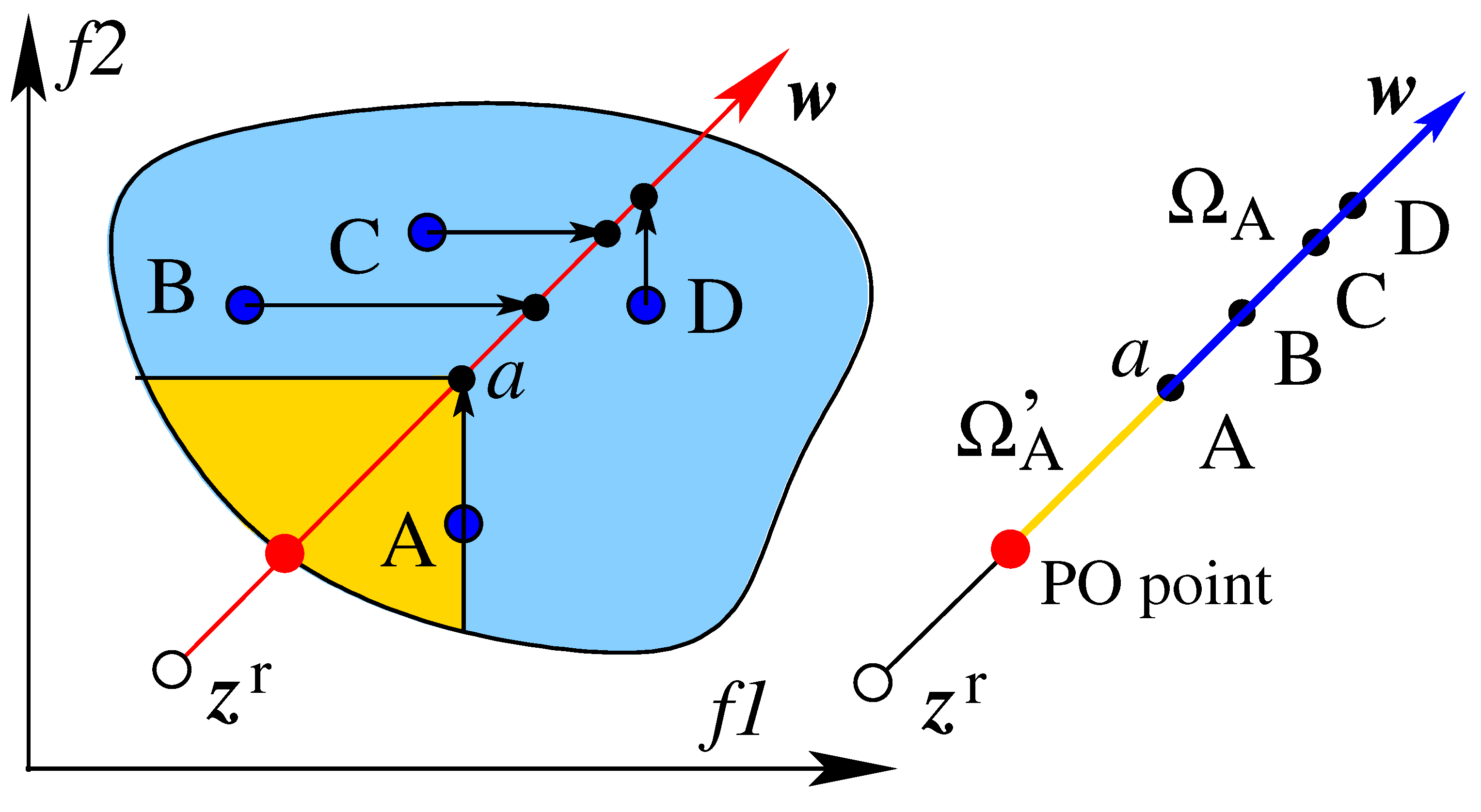
Let us reconsider
Figure 10 with a GD structure with four members in set
P: points O, A, B, and C. The above definition can be used to identify if the point
O is a non-dominated point in
P. There can be two approaches for checking it. First, the
set can be translated to every other feasible point in
P, such as A, B and C, and check if O lies on the respective
set. With three other points in
P, three translations of
are needed. As is clear from
Figure 10, point O does not lie in any of the
sets of three population members. Only at the end of three checks, we know that O is a non-dominated point in
P. The second approach can be executed with the anti-dominance structure and the set
can be put only on
O and check whether any of the other population members lies on the respective
set. It is observed that none of the points (A, B, or C) lie in
, meaning that point O is a non-dominated point in
P. Because the latter involves a single translation of the
set, rather than translating
multiple times, the second approach is a computationally faster non-domination check approach [
16]. In this regard, the creation of
from a given
becomes an important task for non-domination check. On the same account, it is also useful for non-dominated sorting-based algorithms, such as the NSGA series [
16,
17,
18]. The above discussion also results in the following theorem.
Theorem 7 (Identical optimal solution sets). For two identical (or, two identical sets), the respective optimal solution sets are identical.
Proof. Because for a given , is unique and the non-domination check is performed with , if the resulting for two dominance principles are identical, the resulting optimal solution sets will also be identical. □
3.5. Identifying Generalized Optimal Solution Set
If satisfies all three properties (irreflexive, asymmetric and transitive or semi-transitive), then there will exist a non-empty optimal solution set. can be used directly with the following theorem to identify an optimal point:
Theorem 8 (Generalized optimal solution set). A feasible point is optimal with respect to a generalized dominance structure if .
Proof. Because there does not exist any feasible objective vector in the anti-dominance set of in the entire feasible search space , there is no solution to dominate (in the sense of ) it. Hence, is an optimal point. □
The above theorem can be used to achieve the following tasks computationally or theoretically.
First, it can be used to test if an objective vector is a potential optimal point, as discussed above, but instead of restricting the check in a finite sampled set P, every feasible point from the search space must be considered. Although it is a computationally challenging task, the concept can be used theoretically or in a geometry-based checking procedure.
Second, can be used to identify the entire optimal solution set for a given feasible structure . This task will be useful for studies involving test problems and requires an identification of the exact optimal objective set () from for a given dominance structure. The theoretical procedure is to identify set for every point in systematically and by repeating the test only to members in a nested manner. This will allow a faster computational procedure to identify the optimal solution set.
Third, knowing one or more optimal points, can help identify further optimal points quickly by eliminating the dominated solutions from its set and narrowing down the search to find further optimal points. However, in such a task, often the relevant boundary points of can be tested for their optimality. Starting with extreme boundary points of , can immediately verify if the point is a member of the optimal solution set. If yes, the test can continue to the neighboring extreme boundary point, and so on. If no, the test will identify the points in the set that dominate the extreme point and a new test can be executed on members of the set.
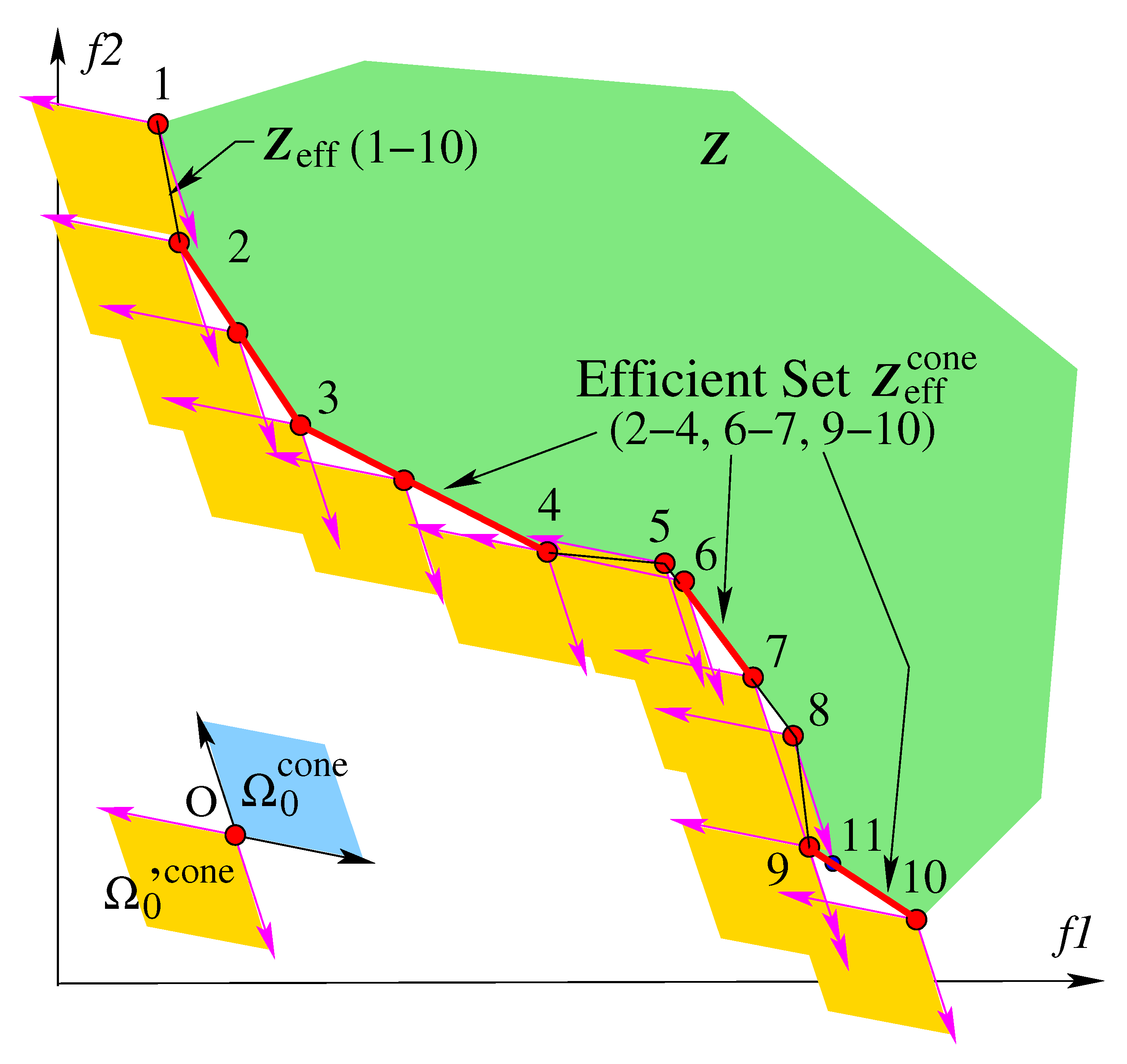
Clearly,
enables a faster way to identify the optimal solution set than
, simply because of the former’s ability to identify points that dominate the current point under consideration, thereby not only allowing to determine if the current point is an optimal point but also narrowing down the search for further optimal points. For the generalized dominance structure (
) shown in the inset of
Figure 11, the resulting
is determined for a hypothetical
, shown in the figure. The
according to the Pareto-dominance principle is the entire line 1–10, whereas the
consists of line segments 2–4, 6–7, and 9–10. For the extreme boundary point 1,
is not empty, as shown by the overlap of
and
at point 1. Thus, point 1 cannot be an optimal point.
also helps to identify the boundary region (line segments between 1 and 10) which must be tested next. Because the relevant boundary in this problem comes from piece-wise linear segments and a cone-dominance structure is used, we restrict our testing only to extreme points of the line segments. By testing point 2 with
, it is clear that
. Thus, point 2 is a member of the optimal solution set. This can continue systematically to identify the entire optimal solution set (line segments 2–4, 6–7, and 9–10). Cone-dominance brings in useful properties, such as, finding
proper Pareto-optimal solutions [
15], finding the partial preferred Pareto set [
1], and helping to eliminate dominant resistant solutions in a population, thereby enabling NSGA-II-like algorithms to solve many-objective problems well [
19].
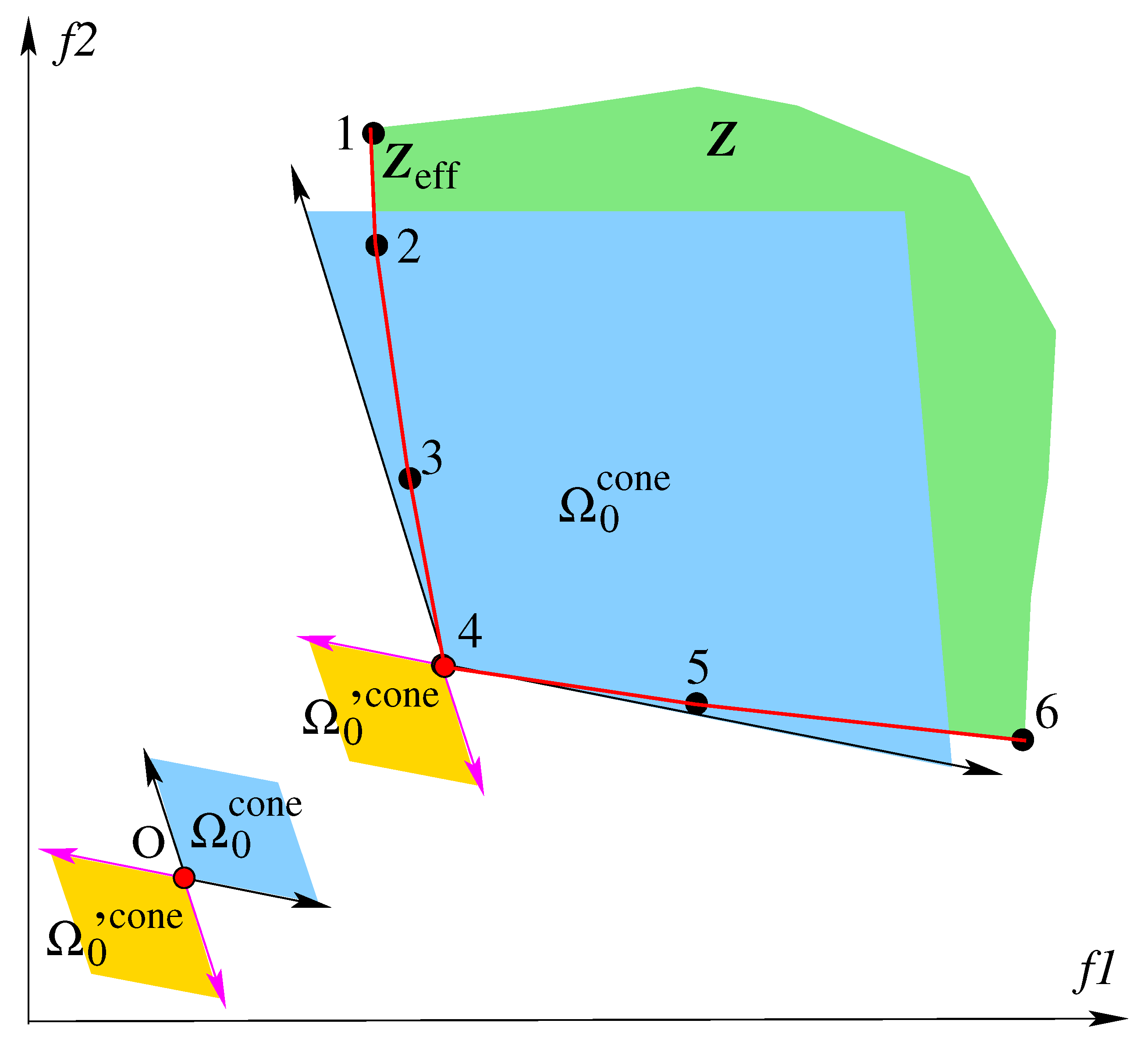
The set at any feasible point can also be used to identify a special scenario:
Theorem 9 (Singleton optimal objective vector). If , then the dominance structure produces a single optimal objective vector for the problem.
Proof. The condition signifies that dominates every point in and thus, no member of dominates . Hence, it is the only optimal point. □
Corollary 4 (Singleton solution). If the condition in the above theorem is satisfied by a unique solution , then is the only strictly optimal solution in the search space.
The single-objective optimality condition satisfies the above condition and results in a singleton global optimal objective value. If the weighted-sum dominance structure, demonstrated in
Figure 9d, satisfies the above condition for a unique solution
, it is the singleton optimal point for the problem [
15].
Figure 12 illustrates one such example.
The following generic properties of dominance structures are also useful for identifying optimal solution sets [
13].
Theorem 10. If is a subset of , then the resulting optimal solution set is a subset of .
Proof. Because , . Thus, every member of that dominates also exists in and dominates . Moreover, there can be additional members of that dominate . Hence, the optimal solution set is a subset of . □
Two corollaries follow from this theorem.
Corollary 5. For any , .
The above corollary means that any dominance structure that is weaker than the Pareto-dominance will include originally dominated points as optimal points, thereby causing a larger optimal solution set. An example is when . The Pareto-optimal set is a subset of the weakly Pareto-optimal set.
Corollary 6. For any , .
The above indicates that any dominance structure that is stronger than the Pareto-dominance structure may not indicate some Pareto-optimal points as optimal, thereby having a reduced number of optimal solutions. An example is when (with an obtuse angle). The cone-optimal set is a subset of Pareto-optimal set .
3.6. Theoretical and Practical Optimal Sets
In addition to identifying the theoretical optimal solution set by the above procedure, there is a practical aspect which we discuss next. For practical reasons, one can define a generalized dominance structure that has an overlapping dominated and anti-dominance sets having
. For such a structure, no theoretical optimal point exists. However, the use of such a dominance structure can still produce artificial optimal points with a multi-objective optimization algorithm due to certain algorithmic inaccuracies and an often-used implementational adjustment. We illustrate these aspects with the epsilon-dominance structure [
20].
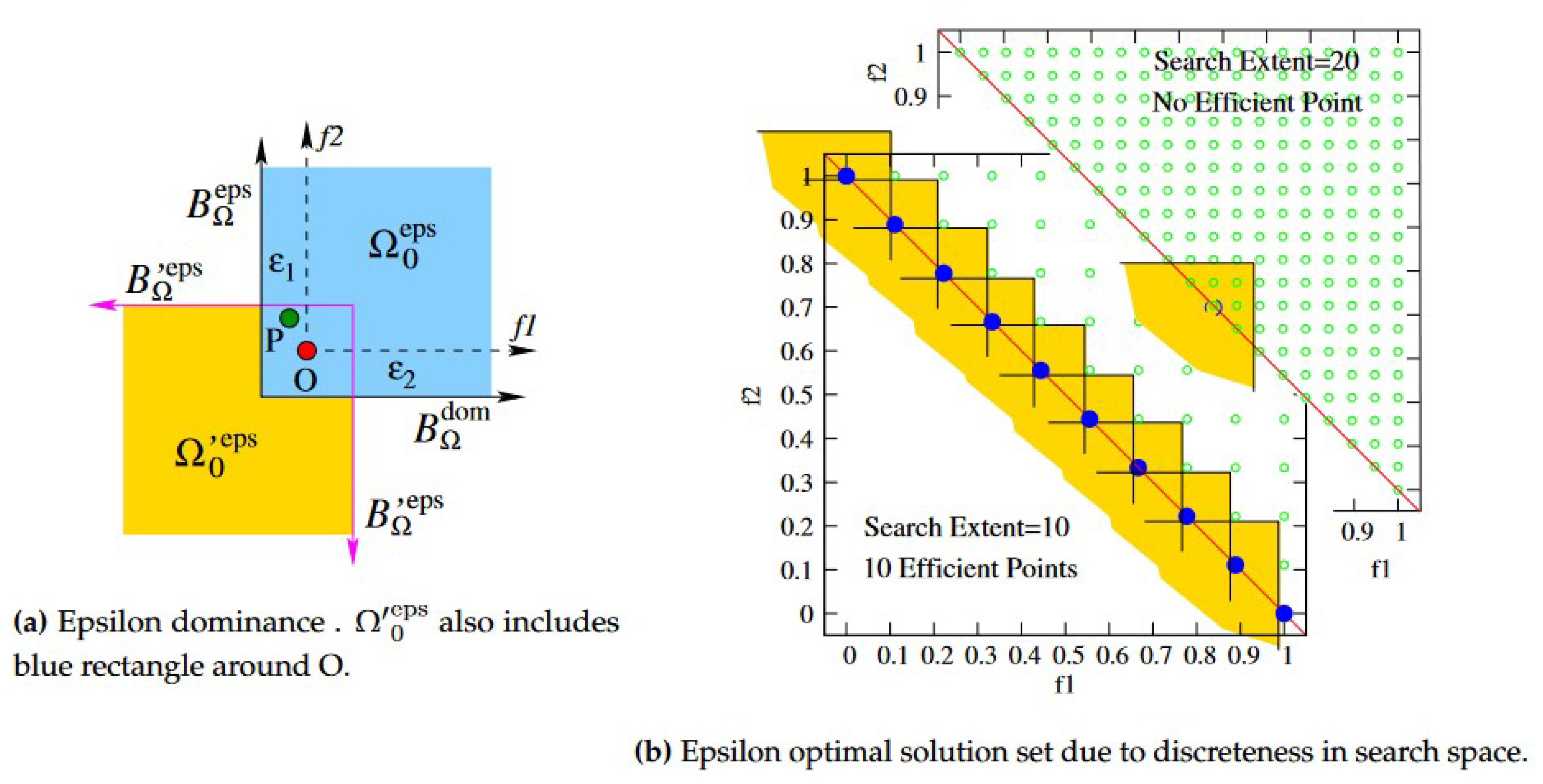
Epsilon-dominance was proposed to obtain Pareto-optimal solutions with a certain pre-specified () difference in the i-th objective values, even in continuous search space problems. The epsilon-dominance structure is defined as follows:
Definition 10 (Epsilon-Dominance).
A feasible solution epsilon-dominates (The original study [20] defined with a product term). Furthermore, notice that this definition is different from epsilon-inferior structure defined in Section 2.1. another feasible solution , if for each . The respective
and
sets are shown in
Figure 13a in blue and golden shaded regions, respectively. It is clear that
, having a small overlapping rectangular region around the point O. Thus, there does not exist a theoretical optimal solution set for this dominance structure. However, an EMO algorithm may still find optimized solutions using this dominance structure but, due to search inefficiencies associated in the algorithm, run for a finite number of solution evaluations. In other occasions, additional implementational changes are forcibly introduced to find a discrete set of optimized solutions with at least
difference in the
i-th objective between any two optimized solutions.
We discuss these ideas, as they can be generically used with some other GD structures.
3.6.1. Search Inefficiency
For a point (say,
) close to the optimal set,
at
indicates the set of points that GD-dominates
. However, if this objective space is relatively small or is difficult to discover by an algorithm’s search operators, the point
may still be declared as an optimal point. Consider point 8 in
Figure 11. It is not an optimal point based on
, due to the existence of a tiny objective space (region 8–9–11). If a multi-objective optimization algorithm fails to find any point in this tiny objective region which would dominate point 8, point 8 will be wrongly declared as an optimal point.
3.6.2. Compatibility of Dominance Structure with Discreteness in Search Space
Artificial optimal points may also emerge if the search space is discrete, causing certain critical points to stay non-dominated due to unavailability of other points in the feasible search space to dominate them.
Figure 13b shows two scenarios with epsilon-dominance structure with
for
to find optimal points for a discrete search space problem on a linear Pareto-optimal front (
for
). In the first scenario (the main part of the figure), each objective value comes at an interval of 1/9. The epsilon-dominance structure finds 10 optimal points, each of whose
is empty, as shown in the figure. Each discrete point clears the
region for other discrete points to constitute 10 optimal points. The second scenario (shown in the inlet figure) has a finer discreteness (
values are available at an interval of 1/19). The inlet figure shows that now no optimal point is discovered, as for every discrete point on the boundary of
, there are a few points in its
set, making it dominated. This example illustrates that despite the non-existence of any optimal solution, a correct combination of the discreteness of the search space and the chosen dominance structure may allow a non-empty optimized solution set to be found.
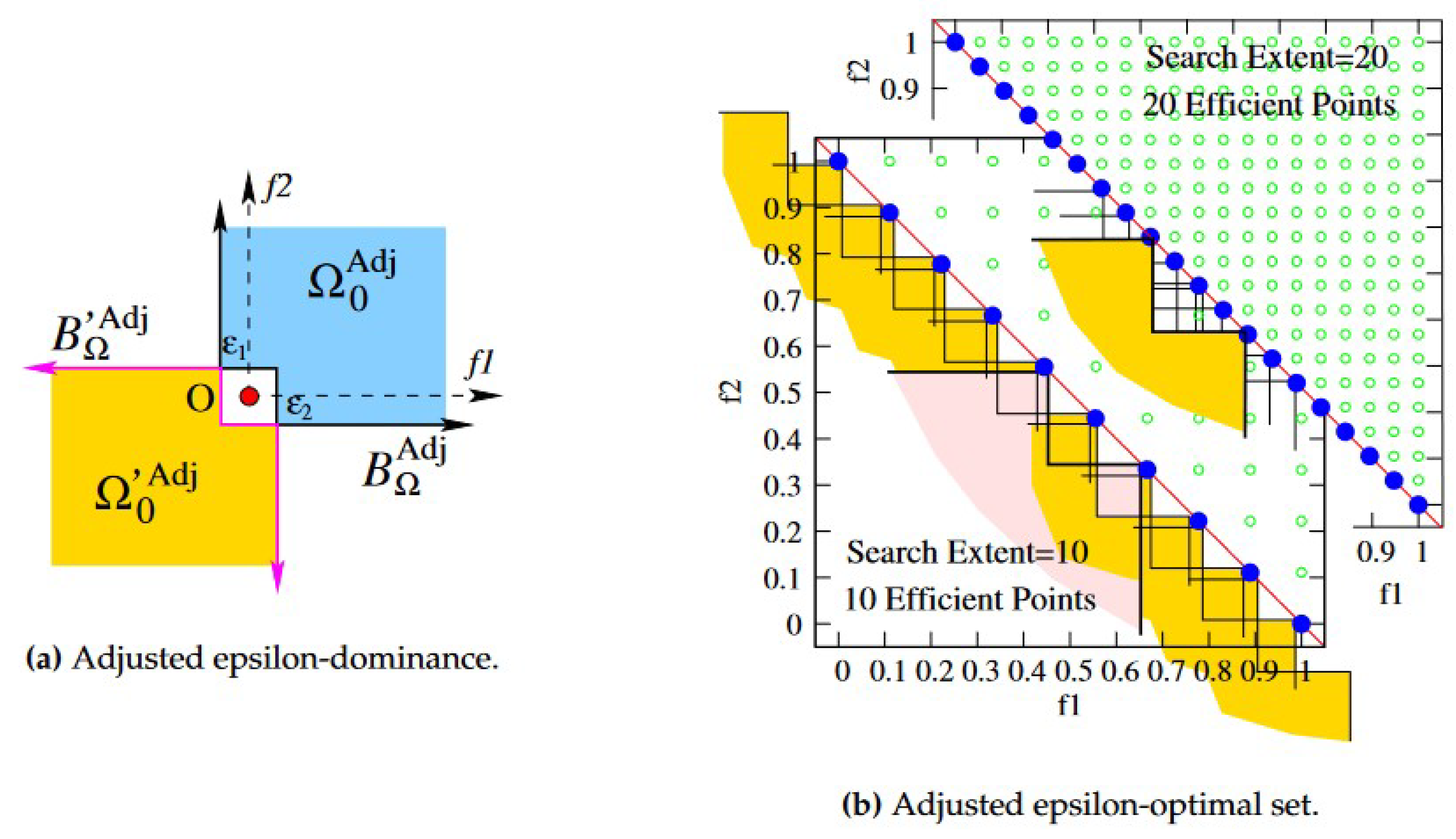
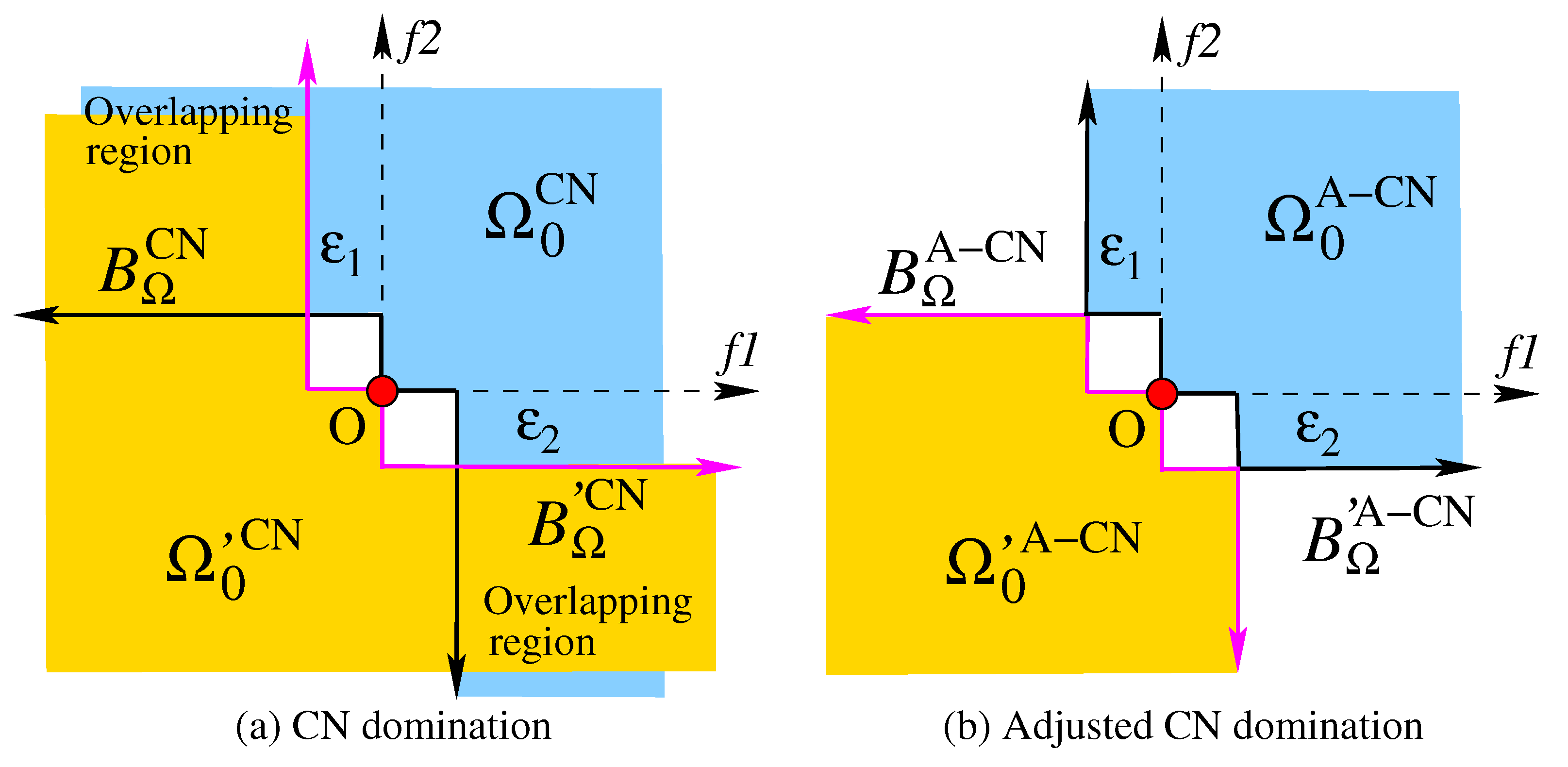
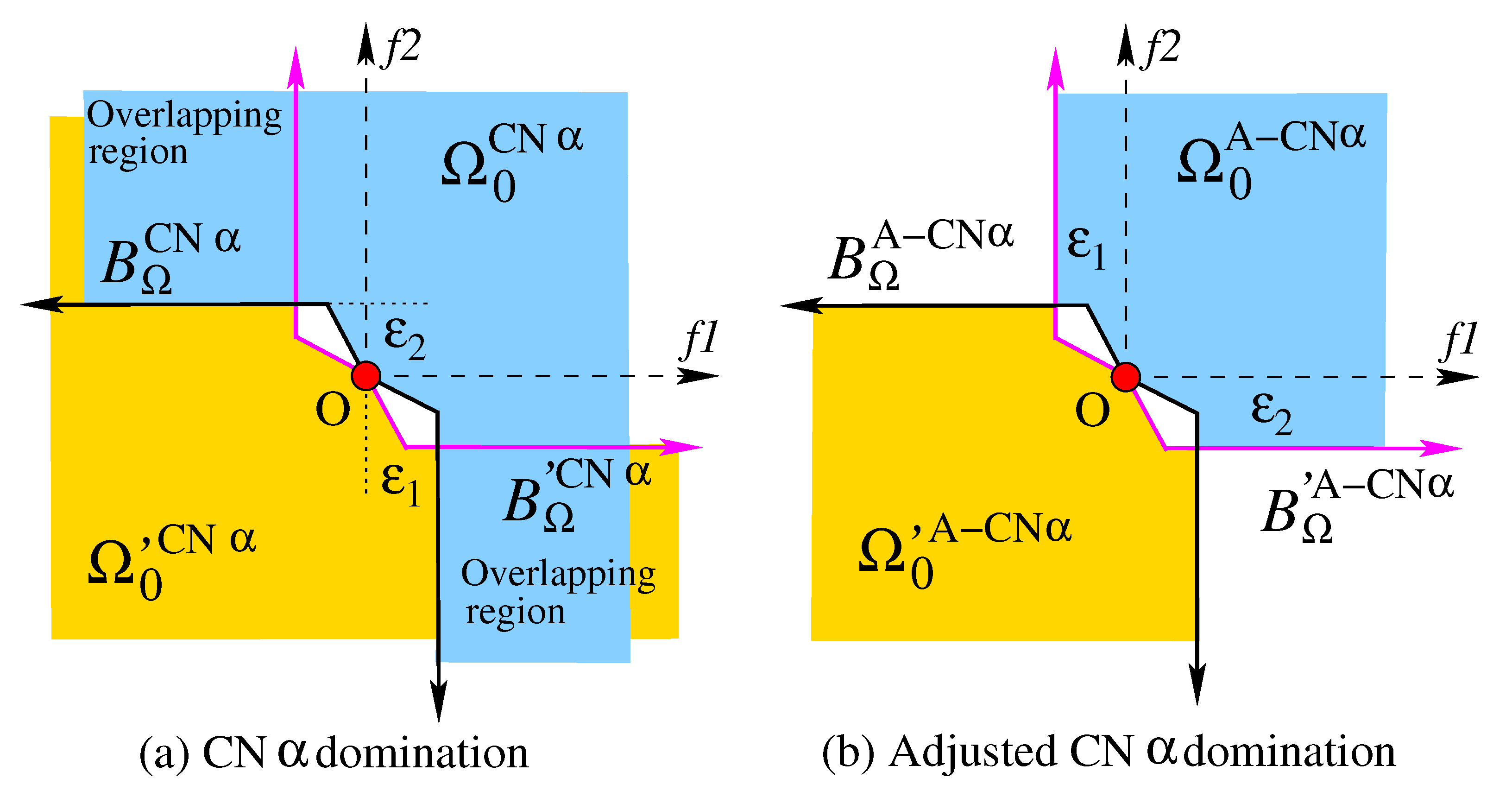
3.6.3. Implementation of Adjusted Dominance Principle
The overlapping dominant structure can be modified before using it in an EMO algorithm so that non-overlapping
and
sets are achieved to produce a non-empty optimal solution set in a problem. For example, the epsilon-dominance structure can be modified by removing the overlapping region between
and
, as follows and as illustrated in
Figure 14a:
The above operations guarantee that adjusted sets are non-overlapping:
.
Figure 14a identifies the same 10 optimal solutions as in
Figure 13b with the above adjusted dominance structure for the coarse search space (interval of 1/9). However, when a finer search space (interval of 1/19) is used, all 20 discrete optimal points are found with the same epsilon vector (
). The non-overlapping property of the adjusted dominance structure discovers a non-empty optimal set, but it seems that the number of optimal solutions cannot be controlled directly by setting the
-vector. The following implementational change fixes this issue.
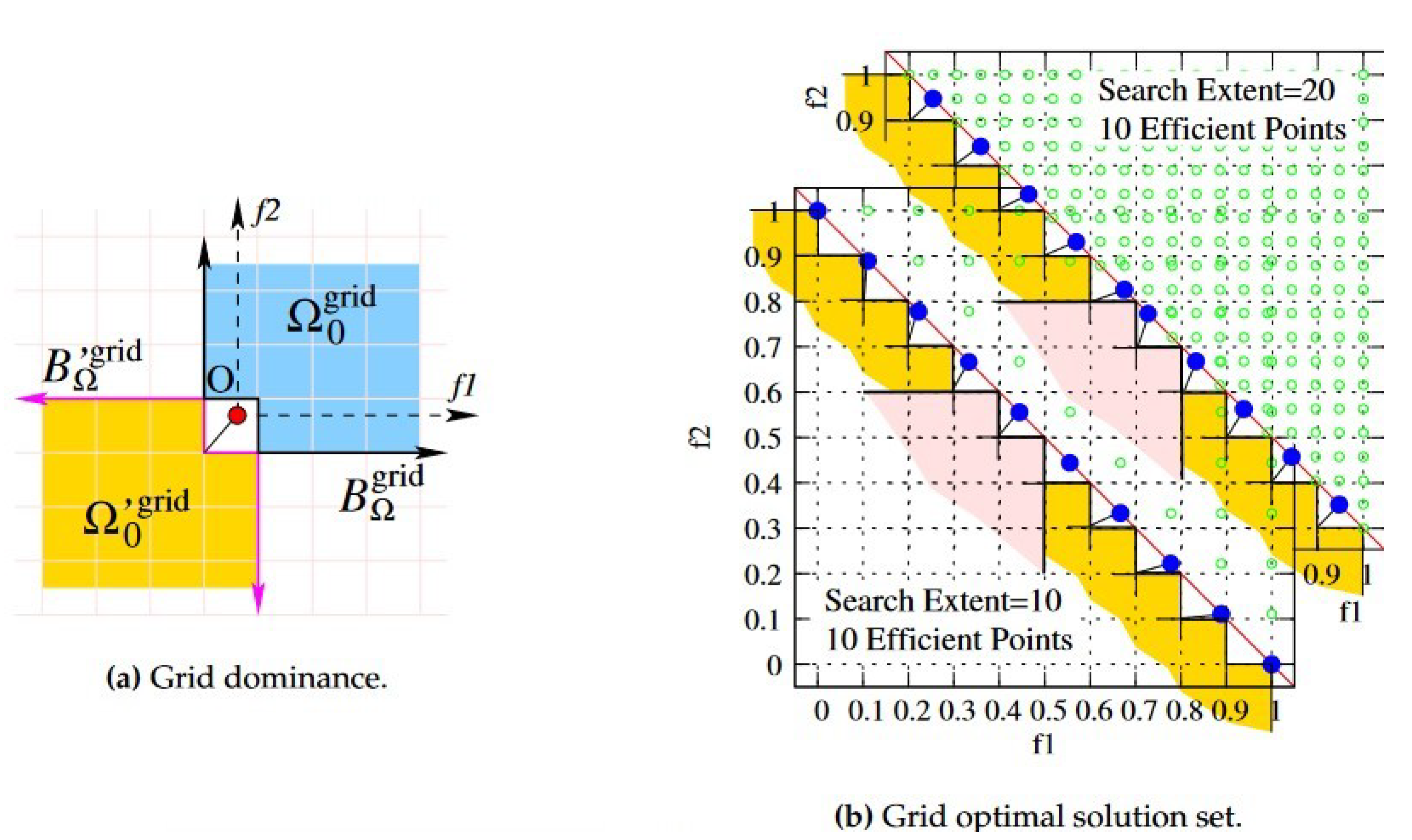
3.6.4. Implementation of Grid Dominance Principle
Another approach adopted by EMO researchers is the use of a fixed grid structure in the objective space with size
along the
i-th objective axis [
21,
22,
23]. Every objective vector
is now replaced with its grid vector (the lower left corner point of the grid in which
lies). In the grid-dominance structure, a Pareto-dominance structure is applied with grid vector of points, and not with the points themselves. If two points in the same grid result in the same grid vector, then the one closer (in the Euclidean sense) to the grid vector dominates the other, as shown in
Figure 15a. Note that the resulting dominance and anti-dominance sets are non-overlapping, or
. This change in the dominance structure produces a non-empty optimal solution set with well-distributed points.
Figure 15b shows that irrespective of the discreteness in the search space, the same number of optimal points are obtained for both levels of discreteness in the search space (interval of 1/9 and 1/19). Because the same epsilon-vector (
) is used in the dominance structure, the final outcomes are identical for both scenarios. Despite the existence of more discrete Pareto-optimal solutions in the search space, the
-vector keeps the cardinality of the optimal set checked.
These algorithmic and implementational adjustments of a generalized dominance structure may produce a different outcome than their Pareto-dominance structure. A proper analysis of the derived for the chosen structure may reveal the expected outcome from an EMO run. Moreover, such a thought process is expected to reveal a better understanding of relationships between and and allow new and innovative dominance structures and new algorithmic implementations to be used for different types of problems.
6. Conclusions
This study has introduced a concept of anti-dominance structure for a chosen static dominance structure by extending the optimality conditions in a single-objective problem to multi-modal problems and then to multi-objective problems. It has been shown that the anti-dominance structure can be useful for identifying the respective non-dominated set in a finite population or perceiving the true optimal solution set in two and three-objective problems. Importantly, the study has brought out certain fundamental principles which every practical dominance structure should have for it to generate a non-empty optimal solution set. However, suitable adjustments to generic dominance structures have been proposed to make them more practically applicable.
To demonstrate their use, dominated and anti-dominance structures have been identified for most popular dominance structures in EMO and classical multi-objective optimization literature. In some situations, an adjustment with mapped objective vectors has been proposed to analyze the resulting optimal solutions. The reasons for their necessary adjustment have been presented in the light of the anti-dominance structures.
It has been shown that with a population-based multi-objective optimization algorithm (such as an EMO algorithm), transitivity of the dominance structure need not be a strict requirement. Semi-transitivity property of dominance structures breaks the cycle of domination among three solutions and allows a transitive relationship to be implicitly formed from the existence of intermediate population members. In this sense, population-based evolutionary multi-objective optimization algorithms have an edge for using more flexible dominated structures possessing semi-transitive properties.
Although not used in this paper, the anti-inferiority concept can be extended to find special and practically relevant (but non-optimal) solutions by developing generalized inferiority conditions for single-objective optimization. An extension of the anti-dominance structure for constrained dominance principles [
47,
48] will motivate further development of optimal constrained multi-objective optimization algorithms. There is a practical need for developing a GUI-based system in which the user can provide any desired dominance structure and the system creates the respective adjusted anti-dominance structure automatically and runs an EMO algorithm with it. This paper has also revealed that for semi-transitive dominance structures, optimization algorithms must find appropriate catalyst intermediate solutions to establish the non-dominated structure. Whether EMO algorithms will be slower in converging to the resulting optimal solution set compared to algorithms which use transitive dominance structures will be an interesting future study. In this regard, it will be interesting to find if there can ever exist a theoretical dominance structure that may cause a domination cycle with four or more solutions. Finally, providing preference elicitation through a number of pair-wise comparisons of objective vectors and creating a meaningful generalized dominance structure from them through the use of developed principles of this paper, would make another interesting practically significant study.


